Brief communication: Growth and decay of an ice stupa in alpine conditions - a simple model driven by energy-flux observations over a glacier ...
←
→
Page content transcription
If your browser does not render page correctly, please read the page content below
The Cryosphere, 15, 3007–3012, 2021
https://doi.org/10.5194/tc-15-3007-2021
© Author(s) 2021. This work is distributed under
the Creative Commons Attribution 4.0 License.

Brief communication: Growth and decay of an ice stupa in alpine
conditions – a simple model driven by energy-flux observations
over a glacier surface
Johannes Oerlemans1 , Suryanarayanan Balasubramanian2 , Conradin Clavuot3 , and Felix Keller4,5
1 Institute
          for Marine and Atmospheric Research, Utrecht University, Princetonplein 5, Utrecht, 3585CC, the Netherlands
2 Department  of Geosciences, University of Fribourg, Fribourg, Switzerland
3 Architecture Clavuot, Gäugelistrasse 49, Chur 7000, Switzerland
4 Academia Engiadina, Samedan, Switzerland
5 Department of Environmental Systems Science, ETH, Zurich, Switzerland

Correspondence: Johannes Oerlemans (j.oerlemans@uu.nl)

Received: 13 February 2021 – Discussion started: 1 April 2021
Revised: 30 May 2021 – Accepted: 4 June 2021 – Published: 29 June 2021

Abstract. We present a simple model to calculate the evo-            to 1 × 10⁶ L. Ice stupas also form interesting touristic attrac-
lution of an ice stupa (artificial ice reservoir). The model is      tions with a distinct and special artistic flavour. They come
formulated for a cone geometry and driven by energy balance          in the same class as ice sculptures, which are popular in all
measurements over a glacier surface for a 5-year period. An          regions of the world that have a cold winter.
“exposure factor” is introduced to deal with the fact that an           The possibility to grow ice stupas of appreciable size de-
ice stupa has a very rough surface and is more exposed to            pends on the meteorological conditions and the availability
wind than a flat glacier surface. The exposure factor enhances       of water. When a surface has a negative energy balance and
the turbulent fluxes.                                                water is sprayed on it, ice will form (a well-known technique
   For characteristic alpine conditions at 2100 m, an ice stupa      to make skating rinks). The more effective the latent heat of
may reach a volume of 200 to 400 m3 in early April. We show          fusion can be removed by contact with cold air and effective
sensitivities of ice stupa size to temperature changes and ex-       emittance of longwave radiation, the faster the ice layer may
posure factor. The model may also serve as an educational            grow. In spring and summer incoming solar radiation will
tool, with which the effects of snow cover, switching off wa-        dominate and the ice stupa will lose mass.
ter during daytime, different starting dates, switching off wa-         In this note we present a model of ice stupa growth and
ter during high wind speeds, etc. can easily be evaluated.           decay, based on a simple consideration of the total energy
                                                                     budget, and driven by energy flux observations over a glacier
                                                                     surface (half hourly observations over a 5-year period). We
                                                                     believe that the energy balance of a glacier surface and of an
1   Introduction                                                     ice stupa have much in common and therefore consider this
                                                                     data set as ideal for a first study. The focus is on alpine con-
Ice stupas (Fig. 1), also referred to as artificial ice reservoirs   ditions at a typical height of 2100 m a.s.l. The purpose of this
(AIRs), are used more and more as a means to store water in          study is to obtain first-order estimates of how fast an ice stupa
the form of ice (Nüsser et al., 2018). In Ladakh, India, engi-       may grow and melt and what processes are most important.
neer Sonam Wangchuk initiated and developed the use of ice           We emphasize that in this note the focus is on the energetics
stupas to provide water for irrigation purposes in spring and        of the ice stupa system, not on the technical aspects that have
early summer. The ice stupas grow in winter by sprinkling            to be dealt with in constructing an ice stupa.
water on the growing ice structure, and they melt in spring
and summer to deliver water; a typical turnover volume is up

Published by Copernicus Publications on behalf of the European Geosciences Union.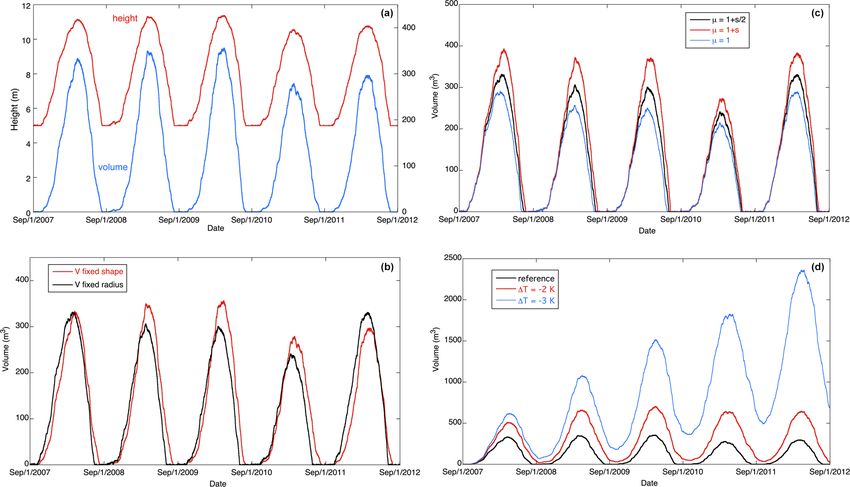
3008                                                J. Oerlemans et al.: Growth and decay of an ice stupa in alpine conditions

Figure 1. (a) Ice stupa in Ladakh, India (courtesy of Sonam Wangchuk). (b) Early growing stage of ice stupa with inner structure in Val
Roseg, Switzerland (courtesy of Conradin Clavuot). (c) Simple geometrical representation. The ice stupa can have an inner structure (brown).
The dashed lines illustrate the growth of an ice stupa from a base with a constant radius.

2   Geometry                                                            of sensible and latent heat. Because of the complex shape of
                                                                        an ice stupa, as compared to a horizontal ice/snow surface, it
Ice stupas have different and often complex shapes. The cone            is hard to describe these processes in detail. However, some
is probably the most appropriate simple geometric shape to              simplifying assumptions may help to arrive at reasonable ap-
represent an ice stupa (Fig. 1), but alternatively a dome (half         proximations.
sphere) could also be considered.                                          We use 5 years of energy balance measurements with an
   The geometric characteristics of a cone with radius r and            automatic weather station (AWS) on the Vadret da Morter-
height h are                                                            atsch (Morteratsch Glacier) (e.g. Oerlemans et al., 2009),
Area of base: π r 2 ,                                         (1a)      which was located at an elevation of about 2280 m a.s.l. The
                 p                                                      surface energy flux is written as
Lateral area: π r r 2 + h2 ,                                  (1b)
                                                                        energy flux = Sin − Sout + Lin − Lout + H + G.                  (4)
             2
Volume: π r h/3.                                              (1c)
                                                                        Sin stands for solar radiation, Sout for reflected solar radia-
  It is useful to introduce a shape parameter s = h/r. The              tion, Lin for incoming longwave radiation, Lout for emitted
volume can then also be written as                                      longwave radiation, H for the total turbulent heat flux, and G
V = π h3 /3s 2 .                                               (2)      for the ground heat flux (conduction from or into the surface
                                                                        layer – generally small compared to the other components).
So for a given volume the height of the ice stupa can be cal-           These quantities are normally expressed in W m−2 . So the
culated from                                                            energy flux is positive when directed towards the surface. A
      3 2 1/3

                                                                        positive energy flux will be used for melting of ice or snow;
h=       Vs      .                                        (3)           when the energy flux is negative freezing of water can take
      π
                                                                        place (when available).
In this note we will consider two cases: (i) the shape factor
                                                                           We now discuss how these measurements over (almost)
is constant during growth and decay, and (ii) the ice stupa
                                                                        flat terrain can be applied to an ice stupa. We first deal
grows upward from a base with a fixed radius, implying that
                                                                        with solar radiation and consider the direct part (fraction q)
the shape factor gradually increases. The first case may be
                                                                        and diffuse part (fraction 1 − q) separately. Although the ra-
more appropriate when an inner structure is used or when
                                                                        tio of direct to diffuse solar radiation depends strongly on
water supply is by varying sprinkler properties or even man-
                                                                        cloud conditions, outside subtropical climate zones where
ually. Case (ii) describes better the situation when a fixed
                                                                        low cloudiness prevails the components are typically of the
spray radius is maintained during the growth phase.
                                                                        same order of magnitude (e.g. Li et al., 2015; Berrizbeitia et
                                                                        al., 2020).
3   Energy exchange                                                        With respect to direct solar radiation, the solar beam can
                                                                        be considered to have a vertical component, impinging on
Ice stupas exchange energy with the surroundings by ab-                 the horizontal surface (base of the ice stupa), and a hori-
sorbing and reflecting solar radiation, absorbing and emit-             zontal component impinging on the vertical cross section (a
ting longwave (terrestrial) radiation, and by turbulent fluxes          triangle). Measurements over a flat surface, like those from

The Cryosphere, 15, 3007–3012, 2021                                                          https://doi.org/10.5194/tc-15-3007-2021
J. Oerlemans et al.: Growth and decay of an ice stupa in alpine conditions                                                       3009

the glacier AWS, thus underestimate the solar radiation in-          value of 2 or more. For a larger shape parameter the exposure
tercepted by an ice stupa. A correction factor f is therefore        will be larger; we therefore use
needed with which the direct radiation as measured by the
AWS has to be multiplied. This factor may be large for a low         µ = 1 + s/2.                                                 (11)
sun, but in alpine conditions where there is always significant
shading by the surroundings this situation is rarely found. A        Equation (9) is no more than an educated guess. It is hard
simple analysis shows that, for a shape factor of s = 2, f           to base estimates of this parameter on information in the lit-
varies from 2.5 for a solar elevation of 20◦ to about 1.2 for a      erature. Many studies have been carried out on the effect of
solar elevation of 60◦ . To account for the fact that the correc-    obstacles on atmospheric boundary layer flow (e.g. trees, but
tion factor should be 1 for a flat surface and increase with the     also buildings), but always in an ensemble setting, looking at
shape factor, we use (note that f and s are dimensionless)           the bulk effect of an ensemble of obstacles. We deal with a
                                                                     case of a single obstacle in open terrain, and we are confident
f = 1 + s/4.                                                  (5)    that the roughness of the surface and the exposure will lead
                                                                     to larger turbulent fluxes. Given the uncertainty in the expo-
For the diffuse part of the solar radiation, illumination is on      sure parameter, later on we will present results for different
all sides and the relevant area therefore is the lateral area as     values.
given in Eq. (1b). Therefore the total amount of absorbed               When water availability is unlimited, the mass gain or loss
solar radiation per unit of time can be estimated as (in J s−1 )     is given by

                                                                     dM/dt = (Fsol + Flw + FL + FH )/Lm + FL /Lv .                (12)
                                                       p
Fsol = f q (Sin − Sout ) π r 2 +(1−q) (Sin − Sout ) π r r 2 + h2 .
                                                              (6)    M is the mass of the ice stupa and Lm is the latent heat
                                                                     of melting/fusion (334 000 J kg−1 ). For typical alpine condi-
Alternatively, one may wish to prescribe the albedo α sepa-          tions the last term in Eq. (10) is normally quite small. Since
rately, i.e.                                                         the volume of the ice stupa is simply related to the mass
                                             p                       (V = M/ρice ), the height of the stupa can directly be calcu-
Fsol = f qSin (1−α)π r 2 +(1−q)Sin (1−α)π r r 2 + h2 . (7)           lated for a given shape factor (case i) or given radius (case ii).
For the longwave radiation and turbulent exchange, the ex-
posed surface is also the lateral area. The longwave radiation       4   Application to the Oberengadin region, Switzerland
balance then becomes
                       p                                             Over the past few years, several ice stupas have been con-
Flw = (Lin − Lout )π r r 2 + h2 .                          (8)       structed in the Oberengadin, southeast Switzerland. In the
                                                                     winter of 2017/2018 an ice stupa was constructed in the Val
   The turbulent heat fluxes depend on the roughness and ex-
                                                                     Roseg at 2000 m a.s.l. (Fig. 1, maximum height about 12 m).
posure of the surface. Since we do not calculate the surface
                                                                     In the winter of 2018/2019 several smaller ice stupas (height
(skin) temperature, we simply assume that it is close to the
                                                                     about 5 m) were built at a site in the Val Morteratsch at about
melting point. The sensible and latent heat input are calcu-
                                                                     1900 m a.s.l. Since February 2021 a test site for ice stupa con-
lated using the well-known bulk transfer equations (e.g. Gar-
                                                                     struction has been in operation at the Diavolezza Talstation
ratt, 1992):
                                                                     at an altitude of 2080 m a.s.l.
                             p                                          To obtain first-order estimates of growth and decay rates
FH = µρcp CU (T − Ts ) π r r 2 + h2                       (9)        for typical climatic conditions in the Oberengadin, we
                                     p
FL = 0.623µρLv CU p−1 (es − e) π r r 2 + h2 .            (10)        used the energy balance measurements from the automatic
                                                                     weather station on the Vadret da Morteratsch as a proxy
Here C is the bulk turbulent exchange coefficient over a flat        for this high alpine region. During the period 1 July 2007–
surface, T is the air temperature, Ts is the surface temperature     30 September 2012, the AWS on the Vadret da Morteratsch
(set to the melting point), ρ is air density, Lv is the latent       was located at an altitude of about 2280 m a.s.l. and has pro-
heat of sublimation (2 830 000 J kg−1 ), cp is the specific heat     duced a unique data set without any gaps. The annual melt at
capacity of air (1004 J kg−1 K−1 ), e is the vapour pressure, es     the AWS location was between 5 and 7 m of ice. With a focus
is the saturation vapour pressure, p is atmospheric pressure,        on the Diavolezza site, which is at an altitude of 2080 m a.s.l.,
and U is the wind speed. The total turbulent heat flux H is          a temperature correction of +1.3 K was applied to the input
just the sum of the fluxes of sensible and latent heat.              data (based on a standard atmospheric temperature lapse rate
   The dimensionless parameter µ is an “exposure/roughness           of 0.0065 K m−1 ). We note that all the locations mentioned
parameter” that deals with the fact that an ice stupa has a          above are within a distance of 10 km from each other (inter-
rough appearance and forms an obstacle to the wind regime.           active map to find locations: https://map.wanderland.ch, last
So µ is expected to be larger than 1 and could perhaps have a        access: 25 June 2021).

https://doi.org/10.5194/tc-15-3007-2021                                                    The Cryosphere, 15, 3007–3012, 2021
3010 J. Oerlemans et al.: Growth and decay of an ice stupa in alpine conditions Figure 2. Energy balance components as measured by the AWS on the Vadret da Morteratsch for January 2008. Net solar radiation in red, net longwave radiation flux in black, turbulent sensible heat flux in blue, turbulent latent heat flux in green. Figure 2 shows an example of data from the AWS. The creases somewhat faster than for the fixed-shape case. Nev- data have been stored as 30 min averages. The turbulent heat ertheless, the differences in the curves are not large and point fluxes have been calculated from the wind speed, air tem- to the fact that in the end the energy constraints determine perature, and humidity, where the turbulent exchange coeffi- how much ice can form (in the case of unlimited water avail- cient C was used as a tuning parameter (to obtain the correct ability). amount of observed ice melt over a 5-year period). The ex- Because the value of the exposure parameter µ is highly ample shown is just for one relatively sunny winter month uncertain, we show the sensitivity of the fixed-radius ice (January 2008). Note the large degree of compensation be- stupa volume to different formulations (Fig. 3c). For µ = 1, tween net solar radiation and net longwave radiation – the implying that the situation is equivalent to that of a flat sur- well-known effect in clear sky conditions on the radiation face, the stupa volume is significantly smaller than in the ref- balance. As a consequence, the turbulent heat fluxes are more erence case (µ = 1+s/2). A stronger dependence of µ on the important than it appears at first sight. shape factor (µ = 1 + s) increases the stupa volume by about Figure 3 summarizes model results in terms of ice stupa 25 %. For a larger shape factor, the mostly negative turbulent height and volume for 5 years. In all calculations we used fluxes in winter increase, and this is not compensated by a q = 0.5 and α = 0.6. It has been assumed that water avail- larger interception of solar radiation. ability is unlimited. In the first example (Fig. 3a) we show In the simulations discussed so far the ice stupas disappear the evolution of an ice stupa on a 5 m high inner structure. in summer. One may ask the question under what conditions In the model this is simply achieved by setting h = 5 m at an ice stupa may survive the summer and grow to a larger size the start of the integration and correct the total volume af- in the next winter. A possible way to study this question is to terwards for the volume of the inner structure. The use of decrease the air temperature uniformly (temperature change an inner structure has the advantage that the freezing area is 1T ). This will imply a stronger negative sensible heat flux in larger from the beginning and that the typical ice stupa shape winter and a weaker positive heat flux in summer, thus accel- is achieved relatively fast. The shape factor has been taken erating stupa growth and slowing down its decay. We found constant and equal to 2. We see some differences among the a break-even point for 1T ≈ −2 K (Fig. 3d). For larger neg- years: the maximum ice stupa height varies between 10 and ative values of 1T the ice stupa does not disappear in sum- 12 m and is normally reached in early April. For the last 2 mer and keeps growing from year to year. For 1T ≈ −3 K, years the simulated ice stupa volume is smaller mainly be- the maximum volume in the fifth year (∼ 2400 m3 ) is about cause of slightly higher temperatures and larger insolation. 4 times that in the first year (∼ 600 m3 ). We note that in this The decay of the ice stupa is hardly faster than the growth. calculation the effect of lower temperatures on the net long- A faster decay would occur if the albedo were not constant wave radiation balance has not been taken into account, be- but would be prescribed to decrease during the melt phase cause the radiation fluxes were prescribed according to the (which is more realistic in most cases). AWS observations. It is likely that we therefore underesti- Figure 3b shows a comparison between the fixed-shape mate the effect of lower air temperature. simulation just described and a fixed-radius simulation with r = 7 m. This value of the radius was chosen to obtain more or less the same ice stupa volume. It can be seen that in the first stage of growth the volume for the fixed-radius case in- The Cryosphere, 15, 3007–3012, 2021 https://doi.org/10.5194/tc-15-3007-2021
J. Oerlemans et al.: Growth and decay of an ice stupa in alpine conditions                                                                3011

Figure 3. Calculated evolution of ice stupa for the case of unlimited water supply for five winters. (a) Height and volume for the case with
an inner structure (height 5 m) and fixed shape. (b) Volume for the case with an inner structure and the case with a fixed radius (7 m). (c) The
effect of the exposure parameter µ on the volume (fixed radius). (d) The effect of a negative temperature perturbation. For 1T = −3 K the
stupa does not disappear anymore but is growing from year to year (fixed shape).

5   Discussion                                                            for the growth phase (e.g. fixed radius) and decay phase (e.g.
                                                                          constant shape factor). Such an approach can easily be ac-
                                                                          commodated in the model.
The data set used to simulate ice stupa growth and decay                     We note that the ice stupa volume calculated here for
for typical conditions in the Oberengadin is probably quite               alpine conditions at ∼ 2100 m a.s.l. (typically 250 m3 ) is sig-
appropriate. The setting of the location of the AWS (on the               nificantly smaller than the volumes obtained in the big ice
lower tongue of the Vadret da Morteratsch when it still ex-               stupas in Ladakh. Winter conditions in Ladakh are consider-
isted) and the Diavolezza Talstation are rather similar: the              ably colder and therefore growth rates can be much larger.
altitude is about the same, and the valley is relatively wide.               In this exploratory study a solid comparison between ob-
However, differences in the wind statistics are likely to exist,          served and simulated stupa sizes was not attempted. How-
but they are difficult to assess. The Morteratsch AWS reveals             ever, we note that the maximum height of the stupa in the
a steady katabatic (glacier) wind most of the time, whereas               Val Roseg was 12 m, which is in good agreement with the
the Diavolezza Talstation is more exposed to the larger-scale             stupa height shown in Fig. 3a.
wind regime. It seems likely that the average wind speed                     The model presented here is simple, basically because we
at the Diavolezza Talstation is somewhat higher than at the               consider the ice stupa to be a single unit with a surface tem-
AWS site, where the 5-year average wind speed is 2.8 m s−1 .              perature close to the melting point. As soon as this constraint
In contrast, the sites in the Val Roseg and Val Morteratsch               is relaxed and the surface temperature of the stupa is con-
are more sheltered and wind speeds are probably lower.                    sidered to be a dependent variable, the whole procedure be-
   The examples presented here are best-case scenarios with               comes more complicated, and some processes can be studied
respect to ice stupa growth. In practice it is not always pos-            more explicitly. Nevertheless, we believe that the simple ap-
sible to have unlimited water availability, and it may be diffi-          proach presented in this note, which requires no more than
cult to sprinkle the water more or less evenly over the stupa,            one page of coding, is a useful tool to obtain first-order es-
especially at higher wind speeds. The choice of the shape of              timates of growth and decay rates under various conditions.
the ice stupa depends on the sprinkling strategy. It may be               Effects of snow cover, switching off water during daytime,
more realistic to describe an ice stupa with different shapes

https://doi.org/10.5194/tc-15-3007-2021                                                           The Cryosphere, 15, 3007–3012, 2021
3012 J. Oerlemans et al.: Growth and decay of an ice stupa in alpine conditions
switching of water supply for high wind speeds, different Review statement. This paper was edited by Chris Derksen and re-
starting dates, differences between warm and cold winters, viewed by Jonathan D. Mackay and two anonymous referees.
etc. can be evaluated. We finally note that the model can eas-
ily be reformulated for another geometry, e.g. a dome.
References
Data availability. The 5-year data set from the weather station on Berrizbeitia, S. E., Cago, E. J., and Muneer, T.: Empiri-
the Vadret da Morteratsch is available on request. cal models of the estimation of solar sky-diffusive radia-
tion. A review and experimental analysis, Energies, 13, 701,
https://doi.org/10.3390/en13030701, 2020.
Author contributions. JO designed, coded, and ran the model. Garratt, J.: The Atmospheric Boundary Layer, Cambridge Univer-
Through their experience in constructing ice stupas, SB, CC, and sity Press, 316 pp., ISBN 0521380529, 1992.
FK have made important contributions concerning the concept and Li, D. H. W., Lou, S. W., and Lam, J. C.: An analysis of global,
application of the model. JO wrote the text of this communication. direct and diffuse solar radiation, Energy Procedia, 75, 388–393,
2015.
Nüsser, M., Dame, J., Kraus, B., Baghel, R., and Schmidt, S.:
Competing interests. The authors declare that they have no conflict Socio-hydrology of artificial glaciers in Ladakh, India: assess-
of interest. ing adaptive strategies in a changing cryosphere, Reg. Env-
iron. Change, 19, 1327–1337, https://doi.org/10.1007/s10113-
018-1372-0, 2018.
Disclaimer. Publisher’s note: Copernicus Publications remains Oerlemans, J., Giesen, R. H., and Van den Broeke, M. R.: Retreating
neutral with regard to jurisdictional claims in published maps and alpine glaciers: increased melt rates due to accumulation of dust
institutional affiliations. (Vadret da Morteratsch, Switzerland), J. Glaciol., 55, 729–736,
2009.
Acknowledgements. We thank the reviewers and editor for their
constructive comments. The operation of the weather station on the
Vadret da Morteratsch was made possible by the NWO-SPINOZA
grant (Dutch Research Council) to Johannes Oerlemans.
The Cryosphere, 15, 3007–3012, 2021 https://doi.org/10.5194/tc-15-3007-2021You can also read