Capital Markets Assumptions 2020 - Envestnet PMC
←
→
Page content transcription
If your browser does not render page correctly, please read the page content below
Capital Markets Assumptions 2020
2020
                                                                                    Capital Markets Assumptions

I. Overview                                                                   The reasoning behind this methodology is to use the
Capital markets assumptions are the expected                                  direction and strength of relationships across various
returns1, standard deviations, and correlation                                asset classes for the common time periods to infer
estimates that represent the long-term risk/return                            what these relationships would have been for the time
forecasts for various asset classes. We use these                             periods, where one of the asset classes does not
values to score portfolio risk, assist advisors in                            have data. In the original methodology all the available
portfolio construction, construct our own asset                               assets are used to construct these cross-asset
allocation models and create Monte Carlo simulation                           relationships. We have improved this methodology
inputs for portfolio wealth forecasts.                                        by utilizing stepwise-fit multivariate linear regression
                                                                              framework (see Glossary of Terms) to guide us in
Our approach to estimating capital markets                                    estimating these cross-asset relationships.
assumptions and constructing asset allocation models
is based on the following general assumptions:                                STEP 2. Theoretical Model: Reverse Optimization
                                                                              To obtain the long-term expected return estimates as
•	The global capital markets are largely efficient in                        implied by the CAPM, we use the reverse optimization
   the long run, where the efficiency of the markets is                       approach proposed by William Sharpe (1974). While
   measured by the Capital Asset Pricing Model (CAPM)                         this approach is based on the same theoretical
   (see Glossary of Terms).                                                   principles as the CAPM, it allows us to avoid
•	While the global capital markets are efficient in the                      estimating the risk premium on the market portfolio.
   long run, there might exist identifiable shorter-term                      Estimating the risk premium on the market portfolio
   inefficiencies in the capital markets.                                     can be a challenging task due to the dependence of
•	Risk premia are time-varying.                                              this estimate on the data period used. Instead, the
                                                                              reverse optimization calls for using (A) the observed
Our capital market assumptions construction process                           market portfolio, (B) market risk aversion coefficient,
is based on using statistically advanced techniques                           and (C) the standard deviations and correlations
to combine information coming from three sources:                             (estimated in Step 1), to obtain the estimates of
theory, researcher views (e.g., forecasts by recognized                       the expected returns. These expected returns, when
economic analysts or our own views into future                                used in conjunction with the standard deviation and
returns of equity and fixed income asset classes), and                        covariance estimates, then imply the observed market
historical data. The process consists of the steps that                       portfolios as the efficient market portfolio under the
are detailed in the next section.                                             CAMP theory.

                                                                              To estimate the observed market portfolio we estimate
II. Process                                                                   the market capitalizations of all the non-overlapping
                                                                              indexes commonly used in constructing long-only
STEP 1: Estimating Standard Deviations and                                    strategic portfolios (see Figure 1). For example, to
Correlations                                                                  estimate the market capitalization of domestic equity
We employ a method created by Robert Stambaugh2                               we look at the market capitalization of Russell’s Top
(1997) to calculate standard deviations and                                   200 Value/Growth, Russell MidCap Value/Growth, and
correlations that are forward looking, in that they                           Russell 2000 Value/Growth indexes.
account for estimation risk (See the Glossary of
Terms). In addition, this estimation method eliminates                        The risk aversion coefficient can be thought of as a
the need to look at only the common data periods                              “magnitude of the trade-off between expected return and
when estimating the standard deviations and                                   variance” (Sharpe, 1974). Instead of trying to estimate
correlations—a common, but a very restrictive way                             this value, we will set this parameter to a value that
to guarantee that correlation matrixes are positive                           makes the rate of return on domestic equity (proxied by
definite3—and allows for the usage of all the available                       Russell 3000 Index) implied by the reverse optimization
data deemed appropriate for a particular asset class.                         equal to the forecast that we make in Step 3.

1
 	The expected returns are given in nominal arithmetic mean terms, although as we note later the translation between nominal vs real and
   arithmetic vs geometric mean returns is straightforward.
2
 	Robert Stambaugh is a professor of finance at The University of Pennsylvania Wharton School.
3
 	See the Glossary of Terms. Also, note that positive definiteness of correlation matrixes is essential when this correlation matrix is used in
   optimization or simulation. Note that a correlation matrix that is obtained from individual pairwise correlations cannot be guaranteed to be
   positive definite.

                                                                          2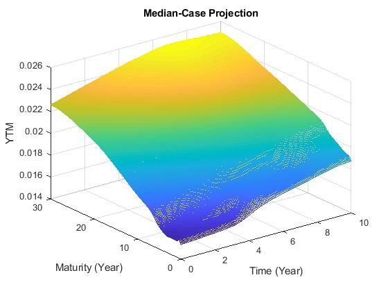
Thus, the reverse optimization framework can be                proxy both empirically and also intuitively is the rate
thought as a way of obtaining the correct relative             of real GDP growth per capita, which under positive
expected return relationships among various assets,            population growth scenario is usually substantially
while the methodology in Steps 3 and 4 (i.e., obtaining        lower than the headline real GDP growth rate. Since
of Researcher Views) guides us in setting the levels of        after the World War II, the real GDP growth has been
these forecasted expected returns.                             almost 3 percent, while the real GDP growth per capita
                                                               has been only slightly above 2 percent. In fact, there
STEP 3. Researcher Views: Equity                               have never been prolonged periods with above 2
We forecast the return for the Russell 3000 Index              percent real GDP per capital growth rates outside of
(which proxies for the entire domestic equity asset            the 1990s, when it averaged 12 percent.
class) and use this estimate as an anchor for the
expected return levels for the other asset classes in          Arnott (2011) notes that while the aggregate real
Step 2.                                                        earnings track the real GDP growth well, the real
                                                               earnings per share grow at a rate that is significantly
Any equity return (both realized and expected) can be          slower than the aggregate real earnings, mainly due
broken down into parts that are attributable to dividend       to a dilution effect. That is, a large part of aggregate
yield and capital gains. Capital gains can be further          earnings growth happens due to growth in new
broken down into a portion that is attributable to the         business, which is not reflected in the existing stock
growth in earnings per share and a portion that is             market indexes.
attributable to growth in P/E ratios. These are exact
algebraic relationships, and if viewed independently           Forecasting the Change in P/E.
of each other do not provide any additional insight for        If the P/E’s are mean reverting, then today’s P/E’s carry
purposes of forecasting. However, if we assume that            information either about future growth of earnings per
pricing multiples (e.g., P/E’s) are mean-reverting (or         share or future returns, or both (Campbell and Shiller,
at least are not likely to stray orders of magnitude           1988). In addition, as shown in Campbell and Shiller
outside historical norms), then, as shown in a seminal         (1998), current P/E’s have a strong negative correlation
paper by Campbell and Shiller (1988), present dividend         with future returns, while at the same time they have
ratios have to forecast either future increases in             practically no correlation with the future earnings per
earnings per share or decreases in future returns. In          share. With the above dynamic relationship in mind,
other words, with this dynamic relationship in place,          high/low levels of current P/E’s can be expected to
we can start tying the three components of the return          correlate to low/high future rates of equity returns (the
(dividend yield, earnings per share growth, and change         most likely mechanism is through multiple repricing)
in P/E ratios) to each other and to the current market         and have negligible forecasting power for the change in
information (e.g., current price multiples and earnings        real per share earnings.
per share growth expectations).
                                                               Thus, to estimate the part of the return that comes
Forecasting the Dividend Yield.                                from P/E’s mean reverting, we look at the current level
As noted by Campbell and Viceira (2005) as well                of Russell 3000 Index P/E and calculate the annual
as Ang and Bekaert (2006), dividend yields follow              rate of return over the next 10 years that will be added
relationships that are almost random walks, which              to/subtracted from the return while the current P/E
means that the best prediction for a future dividend           moves to its long-term mean or “anchor”. For various
yield is today’s dividend yield. Hence, we use the             reasons (see Asness, 2011), P/E multiples from distant
current dividend yield on Russell 3000 index as an             past are not very relevant for calculating this anchor.
estimate for the dividend income part of the nominal           Rather, we form this anchor as a weighted average of
geometric return estimate.                                     the current level of P/E’s and P/E’s going back to early
                                                               1970’s, where the period since 1970’s serves as a
Forecasting the Growth in Earnings Per Share.                  “long-term” horizon.
The nominal growth rate of earnings can be broken
down in two pieces—the expected inflation and the              The reason that we use current level of P/E’s as one
growth rate of real earnings. As noted in Ilmanen              of the components in our P/E anchor calculation is
(2011), it is often mistakenly assumed that the rate           to account for the possibility that the reversion to
of real GDP growth is a good proxy for the growth rate         this anchor from the current P/E levels happens very
of real earnings per share. However, a much better             gradually over time.

                                                           3
Figure 1
2020 World Portfolio n Cash 2.55%
n Commodities 2.12%
n Emerging Markets 5.59%
n High Yield 1.11%
n Int’l Developed Equity 13.15%
n Large Cap Growth 14.45%
n Large Cap Value 12.59%
n Munis 1.58%
n Non-US Fixed Income 19.11%
n Real Estate 1.13%
n Small Cap Growth 0.96%
n Small Cap Value 0.86%
n TIPS 1.50%
n US Fixed Income 23.28%
Grand Total 100.00%
Source: Envestnet | QRG estimate.
On the other hand, the reason for choosing early 1970’s
as the starting point of our long-term horizon is that we
believe financial markets across the world experienced Figure 2
a structural break in 1971, as United States unilaterally
withdrew from the Bretton Woods monetary system,
effectively causing it to collapse. Because of the
breakdown of this system, which essentially allowed
the exchange rates of major economic powers to float
freely against each other, the central banking authorities
were free to engage in inflationary monetary policies,
which they subsequently did. We believe that this ability
on behalf of the central banks to engage in largely
unchecked expansionary monetary policies is one of
the reasons that the P/E’s have been on an upward
trend ever since the beginning of 1970’s with only brief
intermittent pauses and reversals.
Finally, to construct a level of the P/E anchor, where the
base case scenario consists of P/E’s slowly adjusting
towards their long-term anchor from their current levels,
we assign a weight of 70 percent to the current level of
P/E’s and 30 percent to the historical level (since early
1970’s) level of P/E’s.
The last step in estimating the nominal arithmetic
rate of return for Russell 3000 Index is to convert the
nominal geometric rate of return to the arithmetic rate
of return by adding to it half of its variance.
4The following values for the variables of interest were STEP 4. Researcher Views: Fixed Income
estimated: The fixed income expected return forecasting
methodology was developed for the purposes of
• Current Dividend Yield: At the end of March, 2020, informing our Black-Litterman views for the fixed
the dividend yield of the Russell 3000 is forecasted income asset classes (see Envestnet’s white-paper
to be around 1.90%. “Forecasting Constant Maturity Bond Returns”).
• Expected Growth Rate in Real Earnings Per Share: The crux of the methodology is to translate yield-to-
As mentioned earlier, the real GDP growth rate has maturity forecasts into returns on constant maturity
historically formed a ceiling on real earnings per bond portfolios. The methodology serves as an
share growth rate, which is much better tracked interface between the yield-to-maturities, which are
by the growth rate of real GDP per capita and usually the object of forecasts, and the returns on
lower than the real GDP growth rate. To allow for a constant maturity portfolios, which are the values that
possibility of above-average real earnings per share the investors are ultimately interested in. Since the
growth rate, we assume that it will track the real constant maturity bond returns depend on coupon
GDP growth rate over the next decade. payments as well as capital gains, which move in
To obtain the forecast for the real GDP growth opposite directions when the yield curve shifts, the
rate, we survey various professional forecasting calculation of the forecasted total return requires
sources, including: the Congressional Budget Office careful mathematical modeling and analysis.
(CBO), the Federal Open Market Committee (FOMC)
Consensus Forecast, a survey of professional The methodology starts out with a set of yield-to-
forecasters (Philadelphia Fed), the Social Security maturity forecasts for 3 month to 30 year maturity
Administration’s Trustee Report, the IMF World bills and bonds, at various maturity increments, and
Economic Outlook, the World Bank, and others. The at 5- and 10-year forecast horizons. To form our yield
long-term forecast for real GDP growth rate from curve forecasts, we have to take a stance on whether
various sources at the end of March, 2020 was the current forward rates are good forecasts on future
around 1.5 percent. expected yields. If we believe that forwards are good
• Forecasted Inflation: To obtain the inflation forecasts for the expected future yields, we would be
forecast, we survey the same professional taking the position of Pure Expectations Hypothesis,
forecasting sources used to determine the average PEH, which implies that Bond Risk Premium, BRP, is
real GDP growth rate. In addition, we also consider zero. Alternatively, we can make the opposite extreme
market information: the yield spreads between assumption, and assume that yields follow a random
the 10-year nominal Treasury notes and the walk process, which means that the current yields are
inflation-adjusted fixed income securities (TIPS). best predictors of the future yields, and therefore any
These various sources point to expected inflation current yield spread reflects only the required BRP
averaging out at a 2.0 percent level over the next rather than any market expectation for rate changes.
10 years, as calculated at the beginning of 2020.
• Valuation Multiple Adjustment Factor: At the end Researchers have been debating which one of these
of March, 2020, equity P/E ratios are essentially in extremes fit the data best for a long time. For decades
line with the P/E anchor, which we are assuming to data seemed to favor the random walk hypothesis
be their long-term mean reversion level. A P/E ratio (i.e., BRP is positive and yield differences reflect
adjustment from current levels to the “anchor” level mostly the risk premium that is required by the holders
prorated over the next 10 years warrants a -0.05 of longer-term maturity bonds, rather than market’s
percentage point adjustment to the expected return expectations of yield changes), but over the last
of Russell 3000. decade and a half, with BRP hovering around zero, the
• Geometric-to-Arithmetic Rate Conversion: The PEH seems to be making a comeback, as BRPs have
estimated standard deviation for Russell 3000 spiked dramatically since the late summer of 2016, so
Index is 15.23 percent. Thus, this adjustment it might be random walk hypothesis’ time in sun.
factor is equal to 1.16 percent.
We choose not to take a stance in this debate, but
Adding together all the above pieces we get a long-term rather weigh both of these approaches equally by
(10 year) estimate of the nominal arithmetic rate of setting the yield curve forecasts equal to halfway
return for Russell 3000 Index to equal 6.51 percent, between their current level (random walk hypothesis)
which is lower than last year’s 6.82 percent estimate. and those implied by the forward rates (PEH).
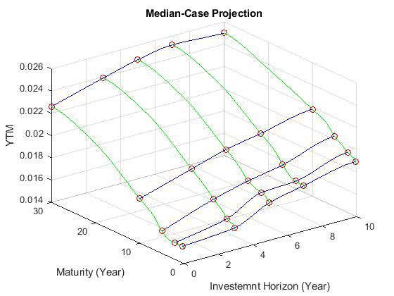
5We then use mathematical smoothing algorithms (e.g., STEP 5. Putting It All Together: Black-Litterman
monotone cubic spline smoothing) to fill in the yield-to- (Bayesian) Process
maturity forecasts for 3 month, 2-, 5-, 10-, and 30-year To obtain our forecasts for the nominal expected
maturity bills and bonds at all the forecast horizons rates of return, we use Black-Litterman (Black &
below 10 years at monthly frequency. Next, we use Litterman, 1991) methodology. The Black & Litterman
Nelson-Siegel method for estimating the complete methodology allows only for combination of expected
yield-curve at a particular forecast horizon. These two returns coming from reverse optimization and the
steps allow us to translate the initial yield-to-maturity views regarding the relative size of future expected
forecasts into a complete yield-to-maturity surface returns of various asset classes. By viewing Black-
with monthly increments in the forest horizons and Litterman methodology as a type of Bayesian
maturities (see Figure 2). approach, we have generalized the methodology to
combine information that comes from the following
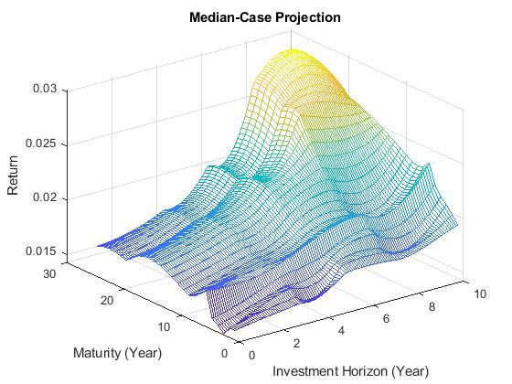
Finally, using the obtained yield-to-maturity surface three sources: theory (reverse optimization, obtained
(Figure 2), we calculate total return on a hypothetical in Step 2), our views about the absolute size of
constant maturity bond portfolio. This is done at a future expected returns (Steps 3 and 4), as well as
range of maturities and investment horizons. Figure historical data.
3 gives the total return surface for the median yield
curve forecast case, and Table 1 gives a subset of the Finally, the Black-Litterman process requires that we
total return outcomes for the bear, median, and bull specify a risk-free rate of return. We use the 10-year
cases at the 10-year forecast horizon. constant maturity Treasury yield to proxy for this, which
at the end of March 2020 was equal to 0.94 percent.
STEP 6: Expected Return Forecasting for Alternative
Figure 3 Asset Classes
To estimate the standard deviations and correlations
of the new alternative asset classes, we use the
approach described in Step 1. Note that this approach
is particularly useful in this instance, since the data
history for the alternative asset classes is relatively
short, when compared to the data histories of the
more traditional asset classes.
The alternative asset classes do not fit into the
reverse optimization and Black-Litterman framework
used for the other asset classes. This is because
the strategies and the funds representing these
strategies invest in the asset classes that are
already represented in the calculation of the
world portfolio in Step 2. Counting the market
capitalization as part of the world portfolio would,
Table 1: Average Returns (10-year forecast)
therefore, result in double-counting and in artificial
Bond Maturity Forecast Made inflation of the world portfolio.
(years) March 26, 2020 December 28, 2018
1 0.67 2.80 Because the alternative asset classes invest in the
3 0.79 2.81 traditional asset classes and therefore cannot be neatly
5 0.90 2.83 folded into our reverse optimization and Black-Litterman
7 1.13 2.94 framework, we use a build-up method to estimate
10 1.11 2.99 their expected returns. More specifically, we estimate
3.10
their historical risk premia and add them back to the
15 1.41
risk-free rate to obtain their expected return forecasts.
20 1.48 3.11
The estimated risk premium of a particular alternative
25 1.57 3.19
strategy (e.g., market neutral or managed futures)
includes not only any inherent risk premium associated
62020
Capital Markets Assumptions
with a particular investment strategy, but also represents the Campbell, John Y. and Robert Shiller, 1988, “The Dividend-
average alpha of the managers in the particular alternative Price Ratio and Expectations of Future Dividends and
strategy. These two parts of the estimated risk premium are Discount Factors.” The Review of Financial Studies, Vol.1/3,
closely linked, since, unlike the traditional asset classes, pp.195-228.
the benchmarks that proxy the alternative asset classes are
comprised of active managers that engage in a particular Campbell, John Y. and Robert Shiller, 1998, “Valuation Ratios
strategy. Since the active management alpha should equal and the Long-Run Stock Market Outlook.” The Journal of
to zero in aggregate, the influence of the individual manager Portfolio Management, Winter, pp.11-26.
alpha on the estimated risk premium should be minimal.
Campbell, John Y. and Robert J. Shiller, 2001, “Valuation
Ratios and the Long-Run Stock Market Outlook: An Update.”
III. Results NBER Working Paper No. 8221.
The main themes for this year’s data are as follows:
Campbell, John Y. and Luis M. Viceira, 2005, “The Term
Due to the worldwide pandemic caused by COVID-19, the Structure of the Risk-Return Trade-Off.” Financial Analysts
financial markets have experienced a sharp correction, which Journal, v.61/1, pp.34-44.
is expected to be followed by a commensurate economic
downturn. Compared to our forecast of expected returns at Fama, Eugene F. and Kenneth R. French, 2002, “The Equity
the beginning of the year, our forward looking expected Premium.” The Journal of Finance, v.LVII/2, pp 637-659.
returns reflect an adjustment in risk premia, which is
anticipated by economic theory: namely, that in the time of Black, Fischer and Robert Litterman, 1991, “Global Asset
financial and economic distress, the risk premia of risky Allocation with Equities, Bonds, and Currencies.” Goldman
assets increase, as the risk aversion of the average investor Sachs Fixed Income Research.
increases.
Grinold, Richard C., Kenneth F. Kroner and Laurence B. Siegel,
On the other hand the risk premia of safe harbor assets, 2011, “A Supply Model of the Equity Premium” in “Rethinking
such as Treasuries and short-term government bonds, the Equity Risk Premium” edited by P. Brett Hammond, Jr.,
decrease, as investors seek refuge from the high volatility in Martin Leibowitz, and Laurence B. Siegel. Research Foundation
the market. Our expected return estimates reflect these two of CFA Institute, pp.53-70.
broad themes, with the expected returns of higher-risk asset
classes, such as equities and fixed income credit asset Ilmanen, Antti, 2011, “Time Variation in the Equity Risk
classes, increasing from their levels at the beginning of the Premium” in “Rethinking the Equity Risk Premium” edited by
year, while those for safer asset classes, such as shorter- P.Brett Hammond, Jr., Martin Leibowitz, and Laurence B. Siegel.
duration bonds, drastically lower from their earlier levels. Research Foundation of CFA Institute, pp.101-116.
Lintner, John. 1965. “The Valuation of Risk Assets and the
IV. References Selection of Risky Investments in Stock Portfolios and Capital
Ang, Andrew and Geert Bekaert, 2007, “Stock Return Budgets.” Review of Economics and Statistics. 47:1, pp.13–37.
Predictability: Is It There?” The Review of Financial Studies,
v.20/3, pp. 651-707. Mossin, Jan. 1966. “Equilibrium in a Capital Asset Market.”
Econometrica, v.34/4. pp.768-783.
Arnott, Robert D., 2011, “Equity Risk Premium Myths” in
“Rethinking the Equity Risk Premium” edited by P.Brett Sharpe, William F. 1964. “Capital Asset Prices: A Theory
Hammond, Jr., Martin Leibowitz, and Laurence B. Siegel. of Market Equilibrium under Conditions of Risk.” Journal of
Research Foundation of CFA Institute, pp.71-100. Finance. 19:3, pp.425–42.
Asness, Clifford, 2011, “Reflections After the 2011 Equity Sharpe, William F., 1974, “Imputing Expected Security
Risk Premium Colloquium” in “Rethinking the Equity Risk Returns from Portfolio Composition.” The Journal of Financial
Premium” edited by P.Brett Hammond, Jr., Martin Leibowitz, and Quantitative Analysis, v.9/3, pp.463-472.
and Laurence B. Siegel. Research Foundation of CFA
Institute, pp.27-31.
7Table 2: Capital Markets Assumptions by Asset Class
2020 Estimates 2019 Estimates Year 2020 vs 2019
expected standard expected standard expected standard
return deviation return deviation return deviation
All Cap Russell 3000 TR USD 6.50% 15.23% 6.82% 15.23% -0.31% 0.00%
Global Equity MSCI World NR USD 6.75% 14.62% 7.07% 14.62% -0.33% 0.01%
Large-Cap Core Russell 1000 TR USD 6.48% 15.07% 6.79% 15.06% -0.31% 0.00%
Large-Cap Growth Russell 1000 Growth TR USD 6.40% 16.70% 6.76% 16.75% -0.37% -0.05%
Large-Cap Value Russell 1000 Value TR USD 6.58% 14.68% 6.81% 14.63% -0.23% 0.05%
Mid-Cap Core Russell Mid Cap TR USD 6.68% 16.73% 7.13% 16.78% -0.44% -0.04%
Mid-Cap Growth Russell Mid Cap Growth TR USD 6.61% 20.24% 7.12% 20.40% -0.50% -0.16%
Mid-Cap Value Russell Mid Cap Value TR USD 6.73% 15.74% 7.13% 15.70% -0.40% 0.03%
Small-Cap Core Russell 2000 TR USD 6.85% 19.54% 7.17% 19.58% -0.32% -0.04%
Small-Cap Growth Russell 2000 Growth TR USD 6.82% 22.64% 7.15% 22.79% -0.32% -0.14%
Small-Cap Value Russell 2000 Value TR USD 6.88% 17.43% 7.19% 17.34% -0.31% 0.09%
Int'l Developed Mkts MSCI EAFE NR USD 7.28% 16.54% 7.63% 16.63% -0.35% -0.09%
Foreign Large Cap Core MSCI EAFE Large NR USD 7.23% 16.67% 7.60% 16.77% -0.37% -0.10%
Foreign Large Cap Growth MSCI EAFE Large Growth NR USD 7.11% 16.89% 7.48% 17.01% -0.36% -0.12%
Foreign Large Cap Value MSCI EAFE Large Value NR USD 7.34% 17.22% 7.72% 17.30% -0.38% -0.08%
Foreign Small Mid Cap Blend MSCI EAFE Mid NR USD 7.44% 16.79% 7.71% 16.88% -0.26% -0.10%
Foreign Small Mid Cap Growth MSCI EAFE Mid Growth NR USD 7.43% 17.82% 7.70% 17.97% -0.27% -0.15%
Foreign Small Mid Cap Value MSCI EAFE Mid Value NR USD 7.47% 16.77% 7.72% 16.79% -0.26% -0.03%
Cash Citi Treasury Bill 3 Mon USD 0.55% 0.59% 2.75% 0.60% -2.20% -0.01%
Intermediate Bond Barclays US Govt/Credit Interm TR USD 1.77% 3.12% 3.24% 3.14% -1.47% -0.03%
Intermediate Muni Barclays Municipal 7 Yr 6-8 TR USD 1.76% 3.54% 2.27% 3.63% -0.51% -0.09%
Long Bond Barclays US Govt/Credit Long TR USD 2.54% 10.40% 4.03% 10.39% -1.49% 0.01%
Long Muni Barclays Municipal TR USD 1.87% 4.03% 2.45% 4.13% -0.58% -0.10%
Short Bond Barclays US Govt/Credit 1-3 Yr TR USD 1.21% 1.46% 2.99% 1.47% -1.77% -0.01%
Short Muni Barclays Municipal 3 Yr 2-4 TR USD 1.44% 1.84% 2.07% 1.86% -0.63% -0.02%
Commodity DJ UBS Commodity TR USD 3.56% 16.52% 5.16% 16.90% -1.60% -0.38%
High Yield Barclays US Corporate High Yield TR USD 6.02% 7.90% 5.19% 7.98% 0.83% -0.08%
International Bond Citi WGBI NonUSD USD 1.15% 8.71% 3.12% 8.76% -1.97% -0.06%
Int'l Emerging Mkts MSCI EM GR USD 8.11% 22.41% 8.85% 22.66% -0.74% -0.25%
REITs FTSE NAREIT All Equity REITs TR 5.85% 16.60% 6.20% 16.65% -0.34% -0.05%
TIPS Barclays US Treasury US TIPS TR USD 1.28% 5.91% 3.24% 6.11% -1.96% -0.21%
Balanced 60% Russell 1000/40% LB Govt/Credit 4.60% 9.33% 5.37% 9.35% -0.77% -0.02%
Interm.
Bank Loan S&P/LSTA Leveraged Loan TR 5.17% 6.12% 4.67% 6.41% 0.51% -0.29%
Emerging-Markets Bond JPM EMBI Global TR USD 4.34% 8.92% 4.57% 9.44% -0.23% -0.51%
Alternative HFRX Global Hedge Fund Index 3.29% 5.54% 5.02% 5.94% -1.73% -0.40%
Equity Market Neutral HFRX EH: Equity Market Neutral Index 0.02% 3.72% 1.67% 3.75% -1.65% -0.04%
Event Driven HFRX Event Driven USD 3.27% 5.85% 4.90% 6.45% -1.63% -0.60%
Hedged Equity HFRX Equity Hedge Index 3.93% 7.28% 5.71% 7.77% -1.78% -0.49%
Bear Market HFRX EH: Short Bias Index -6.02% 11.18% -3.75% 10.66% -2.27% 0.52%
Multi-Strategy HFRI Fund of Funds Composite USD 2.51% 4.85% 4.17% 5.29% -1.66% -0.44%
Alternative Fixed Income category average: Nontraditional Bond 3.09% 2.75% 4.75% 2.90% -1.66% -0.14%
Managed Futures Barclay CTA Index 2.39% 5.21% 4.14% 5.08% -1.74% 0.13%
Long/Short Credit HFRX Fixed Income-Credit TR USD 4.79% 4.56% 6.73% 4.89% -1.94% -0.32%
Global Macro HFRX Macro/CTA 3.36% 7.68% 5.14% 8.00% -1.77% -0.32%
Inverse Inverse -12.91% 25.76% -14.04% 24.98% N/A 0.78%
Leveraged Leveraged 12.58% 26.27% 14.02% 27.05% N/A -0.78%
Inflation 2.00% N/A 2.10% N/A -0.10% N/A
8Stambaugh, Robert F., 1997, “Analyzing Investments Whose Estimation risk. Sometimes also called “parameter
Histories Differ in Length.” Journal of Financial Economics, uncertainty” is the error introduced in portfolio construction
v.45, pp.285-331. process that arises from differences in the values of
forecasted and realized expected returns, standard
deviations, and correlations.
V. Glossary of Terms
Bayesian statistical approach. A statistical framework Expected return. The mean of a probability distribution of
that allows for consistent integration of various sources returns.
of information. A Bayesian approach allows for integration
of data (e.g., returns for an asset class) with external Mean-variance optimization. A method to select portfolio
information, such as uncertainty about the model parameters weights that provides optimal trade-off between the mean
(i.e., mean, standard deviation, correlation, etc.) and other and the variance of the portfolio return for a desired level of
views imposed by an analyst. risk.
Black-Litterman methodology. A Bayesian quantitative model Positive definiteness. A property of correlation matrixes that
that incorporates information coming from the following two guarantees that the variance and standard deviation of any
sources: expected returns of asset classes as predicted by a portfolio constructed using this correlation matrix will be
theoretical model (implemented through reverse optimization) positive.
and the views of an analyst regarding the means of asset
returns. Russell 3000 Index. An index that encompasses the 3,000
largest U.S.-traded stocks, in which the underlying companies
Capital Asset Pricing Model (CAPM). Used to determine a are all incorporated in the United States. Often used as a
theoretically appropriate required rate of return of an asset, benchmark for the entire U.S. stock market.
if that asset is to be added to an already well-diversified
portfolio, given that asset’s non-diversifiable risk. The model Standard deviation. A statistical measure of dispersion
takes into account the asset’s sensitivity to non-diversifiable of the observed return, which depicts how widely a stock
risk (also known as systematic risk or market risk), often or portfolio’s returns varied over a certain period of time.
represented by the quantity beta (ß) in the financial industry, When a stock or portfolio has a high standard deviation, the
as well as the expected return of the market and the predicted range of performance is wide, implying greater
expected return of a theoretical risk-free asset. The CAPM volatility.
was independently authored by Jack Treynor (1961, 1962),
William Sharpe (1964), John Lintner (1965), and Jan Mossin Stepwise-fit multivariate linear regression. A systematic
(1966). method for adding and removing terms in a regression model
based on their statistical relevance. The technique allows
Correlation. A statistical measure of how two securities for the construction of parsimonious models with robust
move in relation to each other. Perfect positive correlation (a explanatory power.
coefficient of +1) implies that as one security moves, either
up or down, the other security will always move in the same
direction. Perfect negative correlation (a coefficient of -1)
means that if one security moves up or down, the negatively
correlated security will always move in the opposite direction.
If two securities are uncorrelated, the movement in one
security does not imply a linear movement up or down in the
other security.
9Disclosure
The information, analysis, guidance and opinions expressed herein are for general and educational purposes only and are not
intended to constitute legal, tax, securities or investment advice or a recommended course of action in any given situation.
Envestnet makes no representation regarding the accuracy or completeness of the information provided. Information obtained
from third party resources are believed to be reliable but not guaranteed. All opinions and views constitute our judgments as of
the date of writing and are subject to change at any time without notice. Past performance is not indicative of future results.
The historical performance shown and expected return does not guarantee future results. There can be no assurance that
the asset classes will achieve these returns in the future. It is not intended as and should not be used to provide investment
advice and does not address or account for individual investor circumstances. Investment decisions should always be made
based on the investor’s specific financial needs and objectives, goals, time horizon, tax liability and risk tolerance. The
statements contained herein are based upon the opinions of Envestnet and third party sources. Information obtained from third
party sources are believed to be reliable but not guaranteed.
An investment in these asset classes is subject to market risk and an investor may experience loss of principal.
About Envestnet®
Envestnet, Inc. (NYSE: ENV)
Envestnet, Inc. (NYSE: ENV) is a leading provider of intelligent systems for wealth management and financial wellness.
Envestnet’s unified technology empowers enterprises and advisors to more fully understand their clients and deliver actionable
intelligence that drives better outcomes and improves lives.
Envestnet Wealth Solutions enables enterprises and advisors to better manage client outcomes and strengthen their practices
through its leading Wealth Management Operating System and advanced portfolio solutions. Envestnet Tamarac provides portfolio
management, reporting, trading, rebalancing and client portal solutions for registered independent advisors (RIAs). Envestnet Data
& Analytics provides intelligent solutions that enable dynamic innovation through its Envestnet | Yodlee platform.
More than 3,500 enterprises and over 92,000 advisors including: 15 of the 20 largest U.S. banks, 43 of the 50 largest wealth
management and brokerage firms, over 500 of the largest Registered Investment Advisors, and hundreds of Internet services
companies leverage Envestnet technology and services.
For more information on Envestnet, please visit www.envestnet.com.
FOR ONE-ON-ONE USE WITH A CLIENT’S FINANCIAL ADVISOR ONLY
© 2020 Envestnet, Inc. All rights reserved. PMC-CMA-0420
10You can also read