Characteristics and Meteorological Factors of Severe Haze Pollution in China

Research Article
Characteristics and Meteorological Factors of Severe Haze
Pollution in China

 Chao He ,1 Song Hong ,1 Hang Mu ,1 Peiyue Tu ,2 Lu Yang ,1 Biqin Ke,1
 and Jiayi Huang 3
 1
 School of Resource and Environmental Sciences, Wuhan University, Wuhan 430079, China
 2
 Faculty of Resources and Environmental Science, Hubei University, Wuhan 430062, China
 3
 Woodsworth College, University of Toronto, M5S 1A9 Toronto, Canada

 Correspondence should be addressed to Jiayi Huang; evelynhuang719@gmail.com

 Received 3 December 2020; Revised 13 May 2021; Accepted 5 June 2021; Published 22 June 2021

 Academic Editor: Herminia Garcı́a Mozo

 Copyright © 2021 Chao He et al. This is an open access article distributed under the Creative Commons Attribution License, which
 permits unrestricted use, distribution, and reproduction in any medium, provided the original work is properly cited.
 A severe haze pollution incident caused by unfavorable weather conditions and a northern air mass occurred in eastern, northern,
 northwestern, and southwestern China from January 15 to January 22, 2018. To comparatively analyze variations in PM2.5 pollution,
 hourly monitoring data and 24 h meteorological data were collected. Air quality observations revealed large spatiotemporal variation
 in PM2.5 concentrations in Handan, Zhengzhou, Xi’an, Yuncheng, Chengdu, Xiangyang, and Jinan. The daily mean PM2.5 con-
 centrations ranged from 111.35 to 227.23 μg·m−3, with concentration being highest in Zhengzhou. Hourly mean PM2.5 concentration
 presented multiple U-shaped curves, with higher values at night and lower values during the day. The ratios of PM2.5 to PM10 were
 large in target cities and the results of multiscale geographic weighted regression model (MGWR) and Pearson correlation coefficients
 showed that PM2.5 had a significant positive or negative correlation with PM10, CO, NO2, and SO2. The concentration of PM2.5 was
 closely related to the combustion of fossil fuels and other organic compounds, indicating the large contribution of secondary aerosols
 to PM2.5 concentrations. The analysis of meteorological conditions showed that low temperature, low wind speed, and high relative
 humidity could aggravate the accumulation of regional pollutants in winter. Northwestern trajectory clusters were predominant
 contributions except in Jinan, and the highest PM2.5 concentrations in target cities were associated with short trajectory clusters in
 winter. The potential sources calculated by Weight Potential Source Contribution Function (WPSCF) and Weight Concentration-
 Weighted Trajectory (WCWT) models were similar and the highest values of the WPSCF (>0.5) and the WCWT (>100 μg·m−3) were
 mainly distributed in densely populated, industrial, arid, and semiarid regions.

1. Introduction A serious haze pollution incident caused by unfavorable
 weather factors and a northern air mass occurred in eastern,
Severe haze pollution events occur frequently in winter in northern, northwestern, and southwestern China from
China and are dominated by PM2.5 (particulate matter with January 15 to January 22, 2018. The most polluted cities were
aerodynamic diameters no larger than 2.5 µm). Particulate Handan, Zhengzhou, Xi’an, Yuncheng, Chengdu, Xian-
matter pollution adversely affects human health and at- gyang, and Jinan. Many studies have presented long-term
mospheric visibility [1–3]. In addition, the direct and in- measurements and analysis of PM2.5 concentrations in
direct radiation lead to climate change and disturb the Handan, Zhengzhou, Xi’an, Yuncheng, Chengdu, Xian-
structure and function of ecosystems [4, 5]. In densely gyang, and Jinan during the last ten years. For example,
populated and industrially developed areas, daily PM2.5 Zhang et al. [6] reported that the chemical composition of
concentrations in winter frequently exceed the Class II PM10, PM2.5, and PM1 varied in Handan from November 16,
category of the National Ambient Air Quality Standards 2015, to March 14, 2016, with serious pollution occurring
(NAAQS, 75 μg m−3). during most of the cold season. A source analysis carried out

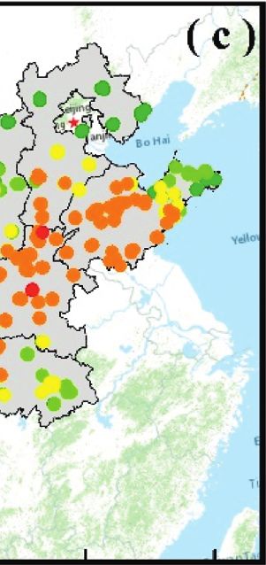
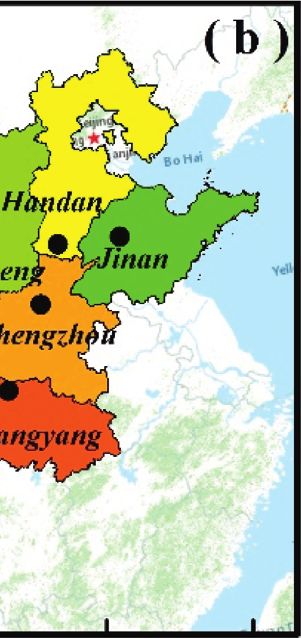
2 Advances in Meteorology

by Jiang et al. [7] with a positive matrix method showed that 2. Methods
the average annual concentrations of PM2.5 and PM10 were
the highest in winter and the lowest in summer. Niu et al. [8] 2.1. Air Quality Observations and Data Quality.
studied the temporal and spatial variation and chemical Observational pollution data from January 15 to January 22,
composition of PM2.5 in the Guanzhong Plain from March 2018, were used in this study. Real-time data were provided
2012 to March 2013. The average daily PM2.5 concentration by the China National Environmental Monitoring Center
was 134.7 μg·m−3, exceeding the Class II category of the (http://www.cnemc.cn) after being validated, with hourly
NAAQS. concentrations of six major pollutants: PM2.5, PM10, sulfur
 Severe atmospheric pollution is closely related not only to dioxide (SO2), nitrogen dioxide (NO2), carbon monoxide
emission sources but also to adverse meteorological condi- (CO), and ozone (O3). We calculated daily mean concen-
tions, terrain, pollutant transport pathways, and chemical trations of PM2.5 in seven cities (Handan, Zhengzhou, Xi’an,
reactions in atmosphere [9–11]. Human activities and mete- Yuncheng, Chengdu, Xiangyang, and Jinan) (Figure 1(b)).
orological conditions are the primary factors leading to var- We used the threshold of 75 μg·m−3 as the highest PM2.5
iation in pollutant concentration [12, 13]. For instance, if the concentration for acceptable air quality according to the
aridity index and average annual temperature increased by 1%, Class II category of the NAAQS (GB3095-2012). Mean PM2.5
PM2.5 concentrations would increase by 66.9 and 35.7, re- concentration in 30 provincial capitals and seven cities was
spectively [14]. But PM2.5-heavy pollution is often accompa- calculated with data from 302 monitoring sites during the
nied by high relative humidity [15, 16]. Moreover, stable pollution period (Figure 1(c)). As shown in Table 1, each city
weather conditions, low temperature, and wind speed can also had set up several air quality monitoring sites, most of which
aggravate the accumulation of regional pollutants in winter. were located in urban areas and some in suburban and rural
PM2.5 and PM10 become very high in the postmonsoon season areas as background sites. Daily mean PM2.5 concentrations
in Kolkata; PM concentrations are observed to be the lowest were calculated when valid data were available for more than
during the monsoon seasons; meanwhile, the NO2 and CO 20 h during the day and values were greater than zero [23].
concentrations demonstrate similar seasonal fluctuations [17]. We adopted the same method as the government reports
 Long-distance transportation among regions also plays daily concentrations of air pollutants to the public, averaging
an important role in PM2.5 pollution. In recent years, the the concentrations at all sites in each city to represent the
Hybrid Single-Particle Lagrangian Integrated Trajectory daily mean concentration of the city.
(HYSPLIT) model and the TrajStat model [18] have become
critical tools for studying long-distance transport and po-
tential pollutant sources. Many scholars have traced the 2.2. Meteorological Data. Hourly meteorological data from
transmission path of CO, O3, SO2, PM2.5, PM10, and other January 15 to January 22, 2018, were obtained from the
gaseous pollutants using HYSPLIT and TrajStat models National Meteorological Information Center of the China
[19–21]. Filonchyk and Yan [22] quantitatively investigated Meteorological Administration (http://data.cma.cn/) and
the causes of severe haze during spring and winter seasons in used to analyze the relationship between meteorological
northwest China based on the backward trajectory and the conditions and air pollution. Hourly meteorological data
HYSPLIT model. The results showed that the movement of included temperature, relative humidity, 2 min wind speed,
air masses in the north, northwest, and west of China is the 2 min wind direction, and sea-level pressure. Mean values of
main cause of haze during spring and winter in northwest each meteorological parameter were calculated using data
China. However, these studies only focused on the transport for all monitoring sites in a region.
direction and passing area in the near surface and did not
carry out statistical analyses of PM2.5 concentrations in
backward trajectories and clustering trajectories. 2.3. Multiscale Geographically Weighted Regression.
 Previous studies have focused on the spatial and temporal MGWR is a significant improvement on GWR because it
distribution of PM2.5 in a single city as well as influence factors allows one to study relationships at varying spatial scales and
and potential sources, which often neglects the impact of covariate-specific bandwidths to be optimized [24]. MGWR
pollutant transport among cities. To better understand the can be defined as
impact of pollutant transport in different cities, real-time y PM2.5 � βbw1 ui , vi PM10i + βbw2 ui , vi SO2i
pollutant data and meteorological data of major Chinese cities
were collected in this research during the haze period in + βbw3 ui , vi COi
January 2018. We investigated the correlations between air + βbw4 ui , vi NO2i + βbw5 ui , vi O3−8hi + εi ,
pollution and meteorological conditions and their spatial (1)
variation. We computed Weight Potential Source Contri-
bution Function (WPSCF) and Weight Concentration- where (ui ,vi ) represents the geographical coordinates of i
Weighted Trajectory (WCWT) models to quantify potential city, βbwi is the regression coefficient, and εi represents a
source distributions in different cities. This research aimed to random error term. We used the MGWR2.2 software to
provide a reference for the local government to manage undertake all calibrations (https://sgsup.asu.edu/sparc/
sudden air pollution incidents, propose a method for studying mgwr). The spatial kernel function type is Bisquare, the
long-distance transport, and identify potential sources of air bandwidth search type is Golden, and the parameter ini-
pollutants in PM2.5 haze pollution. tialization type is GWR estimation [25].

Advances in Meteorology 3

 N

 40°
 50° 0 500 1,000 km

 35°

 40°
 30°
 Latitude (N)

 25°
 30° 100° 105° 110° 115° 120°

 40°
 20°

 35°

 10°
 30°
 Elevation (m)
 High: 6000
 0° Low: –70 25°
 90° 100° 110° 120° 100° 105° 110° 115° 120°
 Longitude (E) Longitude (E)

 PM2.5 (μg m–3)
 350
 116-150
Figure 1: Topography of China (a), locations of the seven polluted cities (b), and the geographical distribution of PM2.5 monitoring stations
in this study (c).

2.4. Trajectory Data. In this study, 72 h backward trajecto- 2.6. Backward Trajectory Statistics and Calculation.
ries arriving at the centers of Handan (114.51°E, 36.62°N), Trajectory cluster calculation was carried out with TrajStat
Zhengzhou (113.64°E, 34.75°N), Xi’an (108.95°E, 34.27°N), [26] http://www.meteothinker.com/downloads/index.html).
Chengdu (104.07°E, 30.66°N), Yuncheng (111.02°E, 35.04°N), TrajStat provides two clustering options, Euclidean distance
Xiangyang (112.17°E, 32.07°N), and Jinan (116.99°E, 36.67°N) or angle distance. In this study, we used angle distance as we
were calculated every 6 h (at 00 h, 06 h, 12 h, and 18 h Co- intended to use the backward trajectories to determine how
ordinated Universal Time) during the pollution period. Data the air mass reached the center of the monitoring point. The
were obtained from the National Centers for Environmental angular distance between two backward trajectories is de-
Prediction (NCEP) reanalysis data and the HYSPLIT model fined as
(version 4.9) developed by the National Oceanic and At-
 1 n A + Bi − Ci 
mospheric Administration Air Resources Laboratory D12 � cos− 1 0.5 i ��� � , (2)
(NOAA ARL, https://ready.arl.noaa.gov/HYSPLIT.php). n i�1 Ai Bi

 where Ai � (X1 (i) − X0 )2 + (Y1 (i) − Y0 )2 , Bi � (X2 (i)
 −X0 )2 + (Y2 (i) − Y0 )2 , and Ci � (X2 (i) − X1 (i))2 + (Y2 (i)
2.5. Inverse Distance Weighted Interpolation. The inverse
 −Y1 (i))2 . D12 is the mean angle between two backward
distance weighted interpolation method is based on the
 trajectories. The variables X0 and Y0 define the position of
principle of similarity. The spatial variation of PM2.5 mass
 the study site.
concentration in China during the pollution period was
drawn in ArcGIS 10.3. We used the coordinate information
of 1,436 air quality monitoring stations in 338 cities as the 2.7. WPSCF Analysis. The Potential Source Contribution
“input point feature” and used daily PM2.5 mass concen- Function (PSCF) algorithm identifies source regions based
tration data at each site as the Z value field. We set the on airflow trajectories analysis and has been widely used to
maximum number of adjacent features and the minimum identify potential source areas for high-concentration pol-
number of adjacent features to 15 and 10, respectively. lutants at receptor sites [27]. The area covered by the

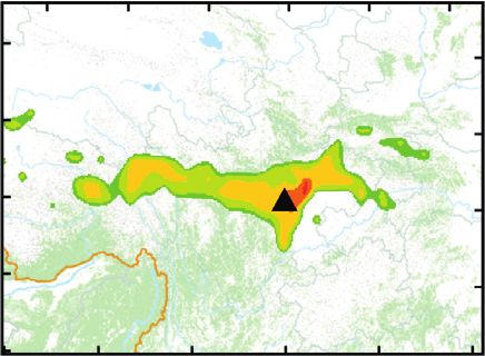
4 Advances in Meteorology

Table 1: Longitude-latitude, regional category, number of background sites, and available monitoring sites of 30 provincial capitals in
China.
City name Longitude Latitude Region Background sites Available sites
Changsha (CS) 112.98 28.20 Central 1 10
Wuhan (WH) 114.29 30.57 Central 1 11
Zhengzhou (ZZ) 113.65 34.76 Central 1 9
Fuzhou (FZ) 119.30 26.08 East 1 7
Hangzhou (HZ) 120.16 30.27 East 1 11
Hefei (HF) 117.28 31.86 East 1 10
Jinan (JN) 117.01 36.67 East 4 15
Nanchang (NC) 115.90 28.68 East 1 9
Nanjing (NJ) 118.77 32.05 East 4 13
Shanghai (SH) 121.47 31.24 East 1 10
Beijing (BJ) 116.38 39.92 North 1 12
Hohhot (HT) 111.66 40.82 North 0 8
Shijiazhuang (SJZ) 114.49 38.05 North 1 9
Taiyuan (TY) 112.57 37.87 North 2 10
Tianjin (TJ) 117.20 39.13 North 1 15
Changchun (CC) 125.32 43.89 Northeast 1 10
Harbin (HB) 126.64 45.74 Northeast 1 13
Shengyang (SY) 123.41 41.80 Northeast 3 13
Lanzhou (LZ) 91.13 29.66 Northwest 1 5
Urumqi (UQ) 87.61 43.79 Northwest 1 8
Xi’an (XA) 108.95 34.26 Northwest 1 13
Xining (XN) 101.79 36.61 Northwest 2 5
Yinchuan (YC) 106.27 38.47 Northwest 1 6
Guangzhou (GZ) 113.26 23.12 South 1 12
Nanning (NN) 108.31 22.81 South 1 8
Chengdu (CD) 104.08 30.66 Southwest 1 9
Chongqin (CQ) 106.51 29.56 Southwest 1 17
Guiyang (GY) 106.71 26.58 Southwest 1 10
Kunmin (KM) 102.70 25.04 Southwest 2 8
Lhasa (LS) 103.75 36.07 Southwest 0 6

backward trajectory is divided into equal i × j grid cells. The 2.8. WCWT Analysis. The PSCF method calculates the
PSCF value for the ijth cell is defined as proportion of pollution trajectories in a grid, reflecting the
 mij potential influence of the grid on the receptor site. Whether
 PSCFij � , (3) pollutant concentrations at the monitoring site are only
 nij
 slightly higher or much higher than the criterion, grid cells
where nij is the total number of trajectory endpoints that fall have the same PSCF value and it can be difficult to dis-
in the ijth grid cells and mij is the total number of trajectory tinguish moderate pollution sources from major sources. In
endpoints for which the monitored pollutant concentration the Concentration-Weighted Trajectory (CWT) method
exceeds a threshold value in the cells (Kong et al., 2013; [28]). [31], each grid cell is assigned a weighted concentration by
In this study, the grid cell size was 0.5°× 0.5 latitude-lon- averaging the sample concentrations that have associated
gitude and we defined 75 μg·m−3 as the threshold value of trajectories crossing that grid cell as follows:
PM2.5 mass concentration. To account for uncertainty, PSCF 1 M
values were multiplied by an arbitrary weight function Wij Cij � cl τ ijl , (5)
 M
 l�1 τ ijl l�1
[29, 30]. The weighting function reduced PSCF values when
the total number of the endpoints in a cell was fewer than where Cij is the average weighted concentration in the ijth
three times the average number of endpoints for all cells. We cell, l is the index of the trajectory, M is the total number of
calculated WPSCF values to identify the possible source trajectories, Cl is the concentration observed on the arrival of
areas of PM2.5 in a region. trajectory l, and τ ijl is the time spent in the ijth cell by
 ⎪
 ⎧ 1.00 nij > 80 ⎫ ⎪ trajectory l. The influence coefficient Wij is also used in the
 ⎪
 ⎪ ⎪
 ⎪
 ⎪
 ⎪ ⎪
 ⎪ WCWT method (WCWTij � Cij × Wij ).
 ⎨ 0.70 20 < n ij ≤ 80 ⎬
 Wij � ⎪ ⎪ ,
 ⎪
 ⎪ 0.42 10 < n ij ≤ 20 ⎪
 ⎪ (4) 3. Results and Discussion
 ⎪
 ⎪ ⎪
 ⎪
 ⎩ ⎭
 0.05 nij ≤ 10
 3.1. Air Pollution Characteristics. In 30 Chinese provincial
 WPSCFij � Wij · PSCFij . capitals during the pollution period, mean concentrations of
 PM2.5, PM10, O3, CO, NO2, and SO2 were 93.7 μg·m−3,

Advances in Meteorology 5

124.2 μg·m−3, 31.6 μg·m−3, 1.5 mg·m−3, 61.6 μg·m−3, and to night in Xi’an and Chengdu, which can be explained by
27.3 μg·m−3, respectively. These results can be explained by the static stability of the atmosphere [38]. During the pol-
the polluted air mass in northern China and adverse weather lution episode, the mean wind speed was 1.65 and 1.62 m·s−1
conditions during the pollution period. Northern cities in Xi’an and Chengdu, respectively, illustrating that the weak
receive relatively weak effects from monsoons, slower wind wind was conducive to the diffusion of pollutants. The
speeds, and small amount of precipitation, resulting in drier temperature was 2.2°C and 9.3°C in Xi’an and Chengdu,
air and more sandstorms, which more often occur in winter, respectively, and relative humidity was 61% and 87%, re-
so it is easier for pollutants to enter the air. In contrast, lower spectively. Thus, low temperature, low wind speed, and high
temperatures are not beneficial to pollutants diffusion, retain relative humidity may have led to the accumulation of PM2.5
pollutants near the surface, and lead to high concentrations in winter.
[32]. A similar phenomenon was observed in the previous High concentrations of PM2.5 appeared at midday (12:
study [33]. Table 2 shows the average concentrations of the 00–13:00) in Handan and Yuncheng (Figure 3(a)), which can
air quality index (AQI) and variations in six major pollut- be explained by high emissions from coal heating, cooking,
ants. The areas with the most severe air pollution and transportation [4, 37, 39]. The lowest PM2.5 concen-
(AQI ≥ 115) were distributed in central, northwestern, and trations were observed in the afternoon, when the boundary
northeastern China. These patterns may be caused by ex- layer becomes larger and the wind speed increased. After 17 :
cessive pollutant emissions from coal-fired heating, biomass 00, PM2.5 concentrations started to increase in Handan,
burning, and industrial combustion in winter [34, 35]. The Zhengzhou, Xi’an, Yuncheng, and Xiangyang because of
AQI of Shijiazhuang, Jinan, Taiyuan, Zhengzhou, Xi’an, and decreasing wind speed and increasing vehicle emissions.
Chengdu reached 170.5, 200.5, 116.2, 260.0, 228.8, and 117.1, PM2.5 pollution emitted from diesel truck traffic, which is
respectively. And the air quality levels reached a moderate or allowed only during nighttime, additionally increased PM2.5
severe pollution grade, which have significant impacts on burden because the emission factors of heavy-duty vehicles
human health. are six times higher than those from light-duty vehicles [40].

3.2. Spatial Analysis of PM2.5. Figure 2 shows the spatial
 3.4. Correlations between PM2.5 and Other Gaseous Pollutants.
distribution of daily mass concentrations of PM2.5 during the
 The Pearson correlation coefficient (r) was used to inves-
pollution period. Elevated concentrations were mainly located
 tigate the relationship between PM2.5 and PM10, CO, NO2,
in central, northwestern, and eastern China and concentrated
 O3, and SO2 using hourly data (Table 3). The analysis results
in southern Hebei, western Shandong, southern Shanxi,
 showed a strong positive correlation (r > 0.9) between PM2.5
northern Henan, central Shaanxi, and central Sichuan because
 and PM10 in the seven polluted cities, indicating that a
of the high emissions from fossil fuel combustion and adverse
 significant fraction of the PM2.5 was secondary PM, such as
weather conditions. Overall, PM2.5 pollution in central and
 ammonium sulfate, secondary organic aerosol, or fugitive
eastern China is more severe than in northern China due to
 dust, which typically have broader regional distributions
distinct emissions sources, weather features, and source ap-
 than anthropogenic primary pollutants [39]. We found large
portionment [36]. PM2.5 pollution in Handan (Hebei Prov-
 values of the ratio of PM2.5 to PM10 in Handan (0.67),
ince), Zhengzhou (Henan Province), Xi’an (Shaanxi
 Zhengzhou (0.79), Xi’an (0.70), Yuncheng (0.65), Chengdu
Province), Yuncheng (Shanxi Province), Chengdu (Sichuan
 (0.68), Xiangyang (0.87), and Jinan (0.64), which indicates
Province), Xiangyang (Hubei Province), and Jinan (Shandong
 the large contribution of secondary aerosols to PM2.5 con-
Province) was highest among major polluted cities, with daily
 centration in these regions. The ratio of PM2.5 to PM10 also
mean PM2.5 concentrations of 212.6 ± 95.5 μg·m−3,
 shows that PM2.5 is the main component of PM10. Similar
227.2 ± 109.9 μg·m−3, 186.7 ± 59.0 μg·m−3, 207.8 ± 83.1 μg·m−3,
 results were reported in the previous study [41]. A positive
111.4 ± 45.4 μg·m−3, 219.3 ± 87.8 μg·m−3, and 163.5 ± 64.7
 correlation between PM2.5 and CO was observed (r > 0.6),
μg·m−3, respectively.
 which revealed that the CO emission process is accompanied
 by the emission of fine particles.
3.3. Daily Mean PM2.5 Concentrations. Daily mean PM2.5 The correlation coefficients between PM2.5 and NO2 and
concentrations in the seven major polluted cities in SO2 in Handan were very high (PM2.5 and NO2: r � 0.88;
Figure 3(b) exceeded the Class II category of the NAAQS. PM2.5 and SO2: r � 0.64). This may be caused by the large
Hourly data were used to examine daily variability in PM2.5 amount of emissions from power plants, urban dust, and the
and identify potential emission sources [37]. Trends in combustion of fossil fuels. In Chengdu, the correlation
hourly mean PM2.5 concentrations in polluted cities were coefficients of PM2.5 with NO2 and SO2 were 0.55 and 0.64,
similar and exhibited multiple U-shaped curves, with higher respectively, mainly due to adverse weather conditions
values in the early morning (0:00–05:00) and at night (19: restricting diffusion and chemical conversion of traffic
00–23:00) and lower values during the middle of the day (12: pollutants. However, correlations between PM2.5 and NO2,
00–15:00). Such daily patterns can be explained by enhanced O3, and SO2 were lower in other cities (Table 3).
emissions from heating, unfavorable meteorological con- To further discuss the relationship between PM2.5 and
ditions, and variations in topography. other pollutants, we investigated the impact of other pol-
 A comparative study of seven major cities found that the lutants on PM2.5 by using the statistical advantage of the
PM2.5 hourly concentrations showed a steady trend from day MGWR model that each regression coefficient was based on

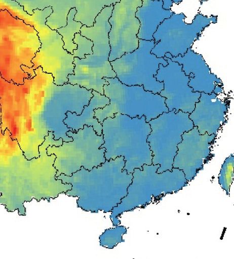
6 Advances in Meteorology

Table 2: Average concentrations of the air quality index (AQI) and six air pollutants in 30 provincial capitals in China during the pollution
period (mg m−3 for CO; μg m−3 for other pollutants).
City AQI PM2.5 PM10 CO NO2 O3_8h SO2
Beijing (BJ) 75.03 42.55 91.24 1.05 52.46 27.06 10.61
Chengdu (CD) 117.11 89.08 128.19 1.27 53.27 27.46 12.10
Fuzhou (FZ) 53.45 35.22 53.56 0.84 35.91 42.41 6.68
Guangzhou (GZ) 133.04 101.02 96.38 1.43 102.50 37.38 16.59
Guiyang (GY) 67.83 48.00 68.60 1.03 34.23 30.58 24.74
Harbin (HB) 99.79 75.54 72.27 1.17 46.61 35.21 45.03
Hangzhou (HZ) 109.93 81.54 115.96 1.12 65.73 17.63 13.84
Hefei (HF) 153.29 125.70 33.67 1.55 67.39 20.87 10.36
Hohhot (HT) 86.74 43.81 119.15 1.64 51.25 33.20 38.17
Jinan (JN) 200.52 156.94 241.90 2.04 80.58 22.21 43.91
Kunming (KM) 59.23 35.50 63.68 0.97 35.55 42.88 17.43
Lhasa (LS) 54.86 27.77 64.50 0.76 29.93 57.49 6.36
Lanzhou (LZ) 99.23 58.35 140.02 1.92 62.70 34.48 41.42
Nanchang (NC) 84.28 61.14 72.75 1.56 47.59 19.40 13.32
Nanjing (NJ) 181.68 141.39 179.42 1.58 79.65 21.33 17.13
Nanning (NN) 105.38 77.01 113.26 1.36 62.86 44.98 16.18
Shanghai (SH) 101.25 76.28 42.54 1.02 71.30 37.25 13.09
Shenyang (SY) 64.44 44.66 67.85 1.19 38.85 25.68 31.91
Shijiazhuang (SJZ) 170.48 133.20 204.43 2.53 68.15 14.46 42.72
Taiyuan (TY) 116.16 77.84 155.67 1.70 58.33 25.58 88.23
Tianjin (TJ) 73.83 50.33 75.41 1.75 41.02 13.88 13.06
Urumqi (UQ) 141.87 151.27 86.59 3.53 65.56 11.84 11.67
Wuhan (WH) 146.77 128.22 35.61 1.53 61.39 17.88 11.03
Xi’an (XA) 228.80 181.62 246.63 2.57 97.20 18.72 32.61
Xining (XN) 86.74 52.42 115.64 2.01 26.05 35.55 22.19
Yinchuan (YC) 57.21 32.64 75.06 1.36 19.01 27.94 29.65
Changchun (CC) 78.70 55.12 69.68 1.09 42.06 33.31 45.43
Changsha (CS) 130.39 124.42 24.44 1.29 49.02 27.88 14.54
Zhengzhou (ZZ) 260.03 222.70 212.38 2.26 83.27 21.02 29.23
Chongqin (CQ) 82.58 61.20 85.42 1.36 43.41 11.77 8.49

 50° 20180115 50° 20180116 50° 20180117 50° 20180118

 40° 40° 40° 40°
 Latitude (N)

 Latitude (N)
 Latitude (N)

 Latitude (N)

 30° 30° 30° 30°

 20° 20° 20° 20°

 80° 90° 100° 110° 120° 80° 90° 100° 110° 120° 80° 90° 100° 110° 120° 80° 90° 100° 110° 120°
 Longitude (E) Longitude (E) Longitude (E) Longitude (E)
 (a) (b) (c) (d)

 50° 20180119 50° 20180120 50° 20180121 50° 20180122

 40° 40° 40° 40°
 Latitude (N)
 Latitude (N)

 Latitude (N)

 Latitude (N)

 30° 30° 30° 30°

 20° 20° 20° 20°

 80° 90° 100° 110° 120° 80° 90° 100° 110° 120° 80° 90° 100° 110° 120° 80° 90° 100° 110° 120°
 Longitude (E) Longitude (E) Longitude (E) Longitude (E)
 (e) (f) (g) (h)
 PM2.5 (μgm–3)

 25 50 75 100 125 150 175 200 225 250 275 300 325 350 375
 −
 Figure 2: Spatial distribution of PM2.5 concentration (μg m 3) in China.

Advances in Meteorology 7

 260 450

 240 400

 220 350

 200 300
 PM2.5 (μg m–3)

 180 250
 200
 160
 150
 140
 100
 120
 50
 100
 0
 0 2 4 6 8 10 12 14 16 18 20 22 24 15 16 17 18 19 20 21 22
 Time (hours) Time (days)
 Handan Chengdu Handan Chengdu
 Zhengzhou Xiangyang Zhengzhou Xiangyang
 Xi’an Jinan Xi’an Jinan
 Yuncheng Yuncheng
 (a) (b)

 Figure 3: Hourly (a) and daily (b) mean PM2.5 concentrations in seven Chinese cities during the pollution period.

 Table 3: Pearson correlation coefficients between PM2.5, PM10, CO, NO2, O3, and SO2 in seven Chinese cities.
 Handan Zhengzhou Xi’an Yuncheng Chengdu Xiangyang Jinan
PM10 0.9787∗ 0.9614∗ 0.9321∗ 0.9880∗ 0.9820∗ 0.9583∗ 0.9416∗
CO 0.8277∗ 0.8594∗ 0.7593∗ 0.6057∗ 0.8068∗ 0.8650∗ 0.7180∗
NO2 0.8818∗ 0.4681 0.4562 0.4373 0.5533∗ 0.4829 0.4970
O3-8h −0.0681 −0.1522 −0.2227 −0.3735 −0.4369∗ −0.0007 0.0873
SO2 0.6386∗ 0.0782 0.3807 0.3695 0.6412∗ 0.1949 0.3145
Note. p < 0.05.

local regression. The model regression results were shown in Table 4: Global regression results of MGWR model.
Tables 4 and 5. In terms of the number of effective pa-
rameters, from the analysis of global regression results, the Descriptive index Value
goodness of fit (R2) was 0.908 (p < 0.05), and the residual Residual sum of squares (RSS) 5.156
sum of squares (RSS) was 51.56 (Table 4). According to the Log-likelihood −12.673
local regression results, the local R2 of all selected cities AICc 517.92
exceeds 0.80 (p < 0.05). These regression results showed that R2 0.908
 Adjust R2 0.889
the MGWR model uses fewer parameters to get the re-
gression results closer to the true value, which could be used
to evaluate the relationship between PM2.5 and other pol- of SO2 is −0.380, p < 0.05), PM2.5 has a significant positive
lutants. It can be clearly found from Table 5 that the rela- correlation with NO2 and SO2.
tionship between PM2.5 concentration and other pollutants
obtained by the MGWR model was similar to that obtained
by the Pearson correlation coefficient. The MGWR analysis 3.5. Meteorological Condition Analysis. The multiscale in-
results showed a strong positive correlation (the regression teraction of meteorological conditions affects air quality in a
coefficient > 1.0, p < 0.01) between PM2.5 and PM10 in the complex way [13]. Previous studies have shown that me-
seven polluted cities. In all selected cities, except Yuncheng teorological factors play an important role in the daily
(regression coefficient is −0.055, p < 0.05), PM2.5 had a variation of pollutant concentrations [13]. The Pearson
significant positive correlation with CO. There was a sig- product-moment correlation coefficient between the hourly
nificant positive correlation between PM2.5 and O3 in mean concentrations of major pollutants and local meteo-
Handan and Zhengzhou, which was contrary to the Pearson rological parameters (wind speed temperature, relative
correlation coefficient. The main reason was that the MGWR humidity, and sea-level pressure) in the seven cities is shown
model was more sensitive to nonlinear relationship than the in Figure 4. In general, the correlation coefficients showed
Pearson correlation coefficient in the regression process. In little difference among cities, indicative of regional pollution
addition, in all cities, except Jinan (the regression coefficient characteristics [20]. PM2.5, CO, PM10, and SO2

8 Advances in Meteorology

 Table 5: Statistical results of MGWR model between PM2.5, PM10, CO, NO2, O3, and SO2 in seven Chinese cities.
 Handan (0.881) Zhengzhou (0.880) Xi’an (0.894) Yuncheng (0.877) Chengdu (0.932) Xiangyang (0.876) Jinan (0.822)
PM10 1.050∗∗ 1.080∗∗ 1.197∗∗ 1.169∗∗ 1.159∗∗ 1.198∗∗ 1.029∗∗
CO 0.151 0.114 0.059∗ −0.055∗ 0.087 0.077∗ 0.191
NO2 0.142∗ 0.148∗ 0.144 0.124 0.197∗ 0.150∗ 0.146∗
SO2 0.354∗ 0.342 0.236 0.239∗ 0.326∗ 0.253 −0.380∗
O3-8h 0.041 0.031∗ −0.040∗ −0.010 −0.021 −0.024 0.047
Note. ∗ , p < 0.05; ∗∗
 , p < 0.01. Numbers in parentheses represent local R2.

 0.6 0.6

 0.4 0.4

 0.2 0.2
 Correlation

 Correlation
 0.0 0.0

 –0.2 –0.2

 –0.4 –0.4

 –0.6 –0.6
 Handan

 Zhengzhou

 Xi’an

 Yuncheng

 Chengdu

 Xiangyang

 Jinan

 Handan

 Zhengzhou

 Xi’an

 Yuncheng

 Chengdu

 Xiangyang

 Jinan
 PM2.5 NO2 PM2.5 NO2
 CO O3_8h CO O3_8h
 PM10 SO2 PM10 SO2

 (a) (b)

 0.6 0.6

 0.4 0.4

 0.2 0.2
 Correlation

 Correlation

 0.0 0.0

 –0.2 –0.2

 –0.4 –0.4

 –0.6 –0.6
 Handan

 Zhengzhou

 Xi’an

 Yuncheng

 Chengdu

 Xiangyang

 Jinan

 Handan

 Zhengzhou

 Xi’an

 Yuncheng

 Chengdu

 Xiangyang

 Jinan

 PM2.5 NO2 PM2.5 NO2
 CO O3_8h CO O3_8h
 PM10 SO2 PM10 SO2

 (c) (d)

Figure 4: The correlation between pollutant concentrations and temperature (a), wind speed (b), relative humidity (c), and sea-level
pressure (d).

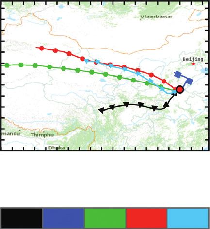
Advances in Meteorology 9

concentrations were positively correlated with temperature space, large numbers of backward trajectories are divided
in Handan, Yuncheng, Chengdu, Xiangyang, and Jinan, into different transport groups or clusters [45]. The calcu-
while O3 concentrations were negatively correlated with lated backward trajectories were divided into five main
temperature in all cities. This can be explained by the fact trajectory clusters from the total spatial variance using the
that solar radiation is the main stimulus for the chemical HYSPLIT and TrajSat models. Main transport pathways
reactions of NO2 and O3 and temperature, which are affected were divided into nine categories according to the results of
by atmospheric turbulence and influence regional pollutant the trajectory clusters (Figure 7): long northwest (LNW:
concentrations [3]. Handan C2, Zhengzhou C3, C4, and C5, Xi’an C2 and C3,
 Generally, pollutant concentrations decrease with in- Yuncheng C2, C3, and C4, Xiangyang C3 and C5, and Jinan
creasing wind speed. Deng et al. [42] and Wang et al. [43] C3 and C4), short northwest (SNW: Xi’an C4 and C5 and
found that low primary pollutant concentrations result in Jinan C1), long north (LN: Handan C3), short north (SN:
high O3 concentrations and cause a positive correlation Handan C4 and C5, Zhengzhou C2, Chengdu C4, and
between wind speed and O3 concentration. We found a Xiangyang C4), short southwest (SSW: Handan C1,
positive correlation between O3 concentration and wind Zhengzhou C1, Xi’an C1, and Jinan C2 and C5), long
speed in Handan, Xi’an, and Jinan (Figure 4(b)). We also southwest (LSW: Yuncheng C1 and C5 and Xiangyang C2),
found a negative correlation between pollutant concentra- long west (LW: Chengdu C1 and C3), short east (SE:
tions and wind speed in Zhengzhou and a positive corre- Chengdu C2), and short south (SS: Chengdu C5 and
lation between PM2.5, CO, PM10, NO2, and O3 with wind Xiangyang C1).
speed in Xi’an, possibly because strong winds can stir up The northwestern trajectory clusters (LNW and SNW)
dust. O3 concentration was weakly positively correlated with passing through some natural sources of aerosol emissions
relative humidity in the seven cities (Figure 4(c)). Primary including northern Xinjiang, southern Inner Mongolia,
pollutant concentrations were negatively correlated with northwestern Gansu, and central Shannxi were predominant
relative humidity in Handan, Yuncheng, Xiangyang, and and accounted for dominant trajectories 72.9%, 55.1%,
Jinan and positively correlated in other cities (Figure 4(c)), 80.2%, 90.6%, 38.5%, and 41.2% of clusters, respectively, in
which indicates that lower relative humidity is unfavorable Handan, Zhengzhou, Xi’an, Yuncheng, Xiangyang, and
for scrubbing gaseous pollutants. Pollutant concentrations Jinan. LW pathways made a large contribution of 53.1% in
were negatively correlated with sea-level pressure in all cities Chengdu. Particle matters accumulated more in short tra-
except Xiangyang, where a positive correlation was ob- jectories. As Table 6 shows, the highest mean PM2.5 con-
served, possibly for two reasons. First, the atmosphere would centrations were associated with SSW (Handan C1, Xi’an
be stable under the low air pressure, leading to the inversion C1, and Jinan C2 and C5), SN (Zhengzhou C2 and Xian-
layer taking place easily and the air convection slowing gyang C4), LSW (Yuncheng C1 and C5), and SS (Chengdu
down, thus resulting in higher concentrations of atmo- C5) pathways. Our results are consistent with those from a
spheric pollutants. The increase in air pressure may have led study from Perrone et al. [46], which found that a longer
to the enhancement of air advection as well as an increase in airflow trajectory had a faster speed not conducive to particle
wind speed, which plays a positive role in the diffusion of air deposition according to the principle of dynamics.
pollutants.
 PM2.5 concentrations in the study cities were influenced
not only by local emissions but also by the surrounding 3.7. Source Analysis. Figures 8 and 9 show the 72 h backward
pollution region. To further study the influence of wind trajectories and potential sources of PM2.5 with WPSCF and
speed and direction on pollutant diffusion, the wind rose and WCWT. The warm-colored areas of the map represent the
the distribution of hourly PM2.5 concentrations, wind speed, main potential sources of pollution that had a significant
and wind direction in the target cities were calculated effect on PM2.5 concentration. The cold-colored regions
(Figures 5 and 6). During the pollution episode, the lowest represent minor potential sources of pollution. Figures 8 and
wind speeds were found in Handan. And the wind speeds 9 show areas with WPSCF > 0.5 and WCWT > 100 μg·m−3
associated with north and northwesterly winds were low in (i.e., where main potential sources were concentrated).
Handan, Zhengzhou, and Yuncheng, while weak winds were PM2.5 pollution in these regions was mainly caused by ar-
associated with the south and southeasterly directions in tificial emissions. In areas with WPSCF < 0.5 and
Xi’an, Chengdu, and Xiangyang. In addition, east winds WCWT < 100 μg·m−3 (i.e., secondary potential sources),
were weak in Jinan (Figure 5). As shown in Figure 6, high PM2.5 pollution was related to the presence of arid and
PM2.5 concentrations were associated with weak winds, less semiarid areas and desert areas, such as the Badain Jaran
than 2–3 m·s−1. Previous studies have shown that low wind Desert, the Ulan Buh Desert, the Kubuqi Desert, and the
speeds can stimulate the accumulation of gaseous pollutants Tengger Desert in Inner Mongolia, where dust storms occur
[44], indicative of the influence of regional transport from frequently [47, 48].
the surrounding polluted regions. The identity and distribution of the main potential
 sources of PM2.5 in each polluted city differed. Our results
 suggest that regional transport from the northwest and south
3.6. Statistical Analysis of Trajectory Clustering. Cluster of Handan plays a dominant role in the formation of pol-
analysis is a widely applied multivariate statistical analysis lution events. Pollution sources were mainly distributed in
technique. According to the similarity principle of trajectory southern Hebei, south of Shanxi, and north of Shaanxi,

10 Advances in Meteorology

 N N N
 40 Handan 50 Zhengzhou 20 Xi’an
 30 NW NE 40 NW NE 15 NW NE
 30

 Wind frequency (%)

 Wind frequency (%)
 20

 Wind frequency (%)
 10
 20
 10 5
 10
 0 W E 0 W E 0 W E
 10 10 5
 20
 20 10
 30
 30 SW SE 15 SW
 40 SW SE SE
 40 Calm:3.125 50 Calm: 1.562 20 Calm:3.646
 S S S
 Wind speed (m/s) Wind speed (m/s) Wind speed (m/s)
 ≥4 1-2 ≥7 3-4 ≥6 2-3
 3-4 0-1 6-7 2-3 5-6 1-2
 2-3 5-6 1-2 4-5 0-1
 4-5 0-1 3-4

 (a) (b) (c)
 N N N
 20 Yuncheng 30 Chengdu 25 Xiangyang
 15 NW NE NW NE 20 NW NE
 20
 15
 Wind frequency (%)
 Wind frequency (%)

 Wind frequency (%)
 10
 10 10
 5 5
 0 W E 0 W E 0 W E
 5 5
 10
 10
 10
 20 15
 15 SW SE SW SE 20 SW SE
 20 Calm:4.167 30 Calm: 1.042 25 Calm: 1.042
 S S S

 Wind speed (m/s) Wind speed (m/s) Wind speed (m/s)
 ≥6 2-3 ≥6 2-3 ≥10 4-5
 5-6 1-2 5-6 1-2 9-10 3-4
 4-5 0-1 4-5 0-1 8-9 2-3
 3-4 3-4 7-8 1-2
 6-7 0-1
 5-6

 (d) (e) (f )
 N
 25 Jinan
 20 NW NE
 15
 Wind frequency (%)

 10
 5
 0 W E
 5
 10
 15
 20 SW SE
 25 Calm: 1.562
 S
 Wind speed (m/s)
 ≥6 2-3
 5-6 1-2
 4-5 0-1
 3-4

 (g)

 Figure 5: Wind rose plots for seven Chinese cities. Calms represent wind speeds

Advances in Meteorology 11

 4.0 8.0 8.0
 Handan Zhengzhou Xi’an

 3.0 6.0 6.0

 Wind speed (m/s)
 Wind speed (m/s)

 Wind speed (m/s)
 2.0 4.0 4.0

 1.0 2.0 2.0

 0.0 0.0 0.0
 0 45 90 135 180 225 270 315 360 0 45 90 135 180 225 270 315 360 0 45 90 135 180 225 270 315 360
 Wind direction (°) Wind direction (°) Wind direction (°)
 3 3 3
 PM2.5 (μgm ) PM2.5 (μgm ) PM2.5 (μgm )

 375 300 225 150 75 0 450 375 300 225 150 75 0 300 225 150 75 0

 (a) (b) (c)
 6.0 6.0 12.0
 Yuncheng Chengdu Xiangyang

 4.5 4.5 9.0
 Wind speed (m/s)
 Wind speed (m/s)

 Wind speed (m/s)
 3.0 3.0 6.0

 1.5 1.5 3.0

 0.0 0.0 0.0
 0 45 90 135 180 225 270 315 360 0 45 90 135 180 225 270 315 360 0 45 90 135 180 225 270 315 360
 Wind direction (°) Wind direction (°) Wind direction (°)
 PM2.5 (μgm3) PM2.5 (μgm3) PM2.5 (μgm3)

 375 300 225 150 75 0 150 75 0 450 375 300 225 150 75 0

 (d) (e) (f )
 6.0
 Jinan

 4.5
 Wind speed (m/s)

 3.0

 1.5

 0.0
 0 45 90 135 180 225 270 315 360
 Wind direction (°)
 PM2.5 (μgm3)

 300 225 150 75 0

 (g)

Figure 6: Distribution of PM2.5 concentrations with observed hourly wind direction and speed in each direction in seven Chinese cities.

distributed around Xi’an and were caused by motor vehicle Chengdu were located in surrounding areas due to unfa-
emissions, thermal power plants, and coal burning for vorable meteorological conditions in winter. High WPSCF
heating in winter. Ningxia and Gansu may also be important and WCWT values were mainly concentrated in the south of
potential sources of PM2.5 pollution in Xi’an since these Henan where population density and biomass burning are
areas are the main sources of dust in winter. Central Gansu, high. The high potential source regions for Jinan were
Ningxia, and Shaanxi were the main potential sources of distributed in southwestern Shandong, northeastern Henan,
pollution in Yuncheng. The high potential source regions for east of Shandong, and south of Hebei [50].

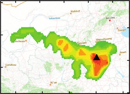
12 Advances in Meteorology

 48° 50° Zhengzhou 46°
 Handan Xi’an
 44° 44° 42°

 Latitude (N)
 Latitude (N)

 Latitude (N)
 38° 38°
 40°
 34°
 36° 32°
 30°
 26°
 32°
 100° 104° 108° 112° 116° 120° 84° 90° 96° 102° 110° 118° 86 90° 94° 98° 104° 110°
 Longitude (E) Longitude (E) Longitude (E)
 Cluster Cluster Cluster

 C1 C2 C3 C4 C5 C1 C2 C3 C4 C5 C1 C2 C3 C4 C5

 (a) (b) (c)
 46° 40° 44°
 Yuncheng Chengdu Xiangyang
 42° 36° 40°

 Latitude (N)

 Latitude (N)
 Latitude (N)

 38° 36°
 32°
 34° 32°
 28°
 30° 28°
 24°
 86 90° 94° 100° 106° 112° 88° 92° 96° 100° 104° 108° 88° 92° 96° 102° 108° 114°
 Longitude (E) Longitude (E) Longitude (E)
 Cluster Cluster Cluster

 C1 C2 C3 C4 C5 C1 C2 C3 C4 C5 C1 C2 C3 C4 C5

 (d) (e) (f )
 46° Jinan

 42°
 Latitude (N)

 38°

 34°

 30°

 102° 108° 114° 120° 126°
 Longitude (E)
 Cluster

 C1 C2 C3 C4 C5

 (g)

 Figure 7: Spatial distribution of cluster means in seven Chinese cities, with the large red dots representing cities.

Table 6: Mean backward trajectory clusters frequency (%) and PM2.5 mean concentrations (μg m−3) associated with the five trajectory
clusters in seven Chinese cities. Bold numbers represent the mean PM2.5 concentration of each trajectory cluster.
City Cluster1 (C1) Cluster2 (C2) Cluster3 (C3) Cluster4 (C4) Cluster5 (C5)
 12.50 72.92 8.33 4.17 2.08
Handan
 304.00 207.99 109.92 227.69 211.25
 10.42 12.50 38.54 21.88 16.67
Zhengzhou
 255.14 270.89 208.07 330.65 205.90
 19.79 12.50 35.42 15.63 16.67
Xi’an
 200.36 182.73 192.90 198.91 164.13
 5.21 17.71 35.42 37.50 4.17
Yuncheng
 235.56 233.98 191.93 200.75 228.65
 11.46 32.29 41.67 7.29 7.29
Chengdu
 112.90 119.31 120.79 98.50 135.93
 8.33 34.38 23.96 18.75 14.58
Xiangyang
 198.17 208.89 192.95 261.73 261.04
 6.25 14.58 62.50 7.29 9.38
Jinan
 162.11 183.07 189.33 143.35 191.00

Advances in Meteorology 13

 42°
 46° Handan Zhengzhou Yuncheng
 42° 38° Xi’an
 39°
 Latitude (N)

 Latitude (N)

 Latitude (N)

 Latitude (N)
 42°
 39° 36°

 38° 34°
 36° 36°

 34° 33° 32°
 33°

 94° 100° 106° 112° 118° 96° 102° 108° 114° 102° 106° 110° 114° 100° 104° 108° 112°
 Longitude (E) Longitude (E) Longitude (E) Longitude (E)
 (a) (b) (c) (d)

 36° Chengdu Xiangyang Jinan
 36° 40°
 Latitude (N)

 Latitude (N)

 Latitude (N)
 33° 38°
 33°
 30° 36°
 30° 34°
 27°

 92° 96° 100° 104° 108° 112° 102° 105° 108° 111° 114° 106° 110° 114° 118° 122°
 Longitude (E) Longitude (E) Longitude (E)
 (e) (f) (g)
 WPSCF

 0.3 0.4 0.5 0.6 0.7 0.8 0.9 1.0

Figure 8: Potential sources of PM2.5 in seven Chinese cities according to the Weight Potential Source Contribution Function (WPSCF), with
the large black triangles representing cities.

 42° 42°
 Handan 40° Zhengzhou Xi’an Yuncheng
 38°
 38° 40°
 Latitude (N)

 Latitude (N)

 Latitude (N)

 Latitude (N)
 39° 36°
 36° 38°
 34° 36°
 34°
 36°
 32° 32° 34°

 105° 108° 111° 114° 117° 104° 108° 112° 116° 102° 104° 106° 118° 110° 112° 100° 104° 108° 112°
 Longitude (E) Longitude (E) Longitude (E) Longitude (E)
 (a) (b) (c) (d)

 34° Chengdu 36° Xiangyang 40° Jinan

 34° 38°
 Latitude (N)

 Latitude (N)

 Latitude (N)

 32°
 32° 36°
 30° 30° 34°
 28° 32°
 28°
 102° 104° 106° 118° 110° 106° 110° 114° 118° 108° 112° 116° 120°
 Longitude (E) Longitude (E) Longitude (E)
 (e) (f) (g)
 WCWT (μgm–3)

14 Advances in Meteorology

Handan, Xi’an, Zhengzhou, and Yuncheng and PM2.5, PM10, the National Academy of Sciences, vol. 110, no. 32,
CO, and SO2 concentrations were positively correlated with pp. 12936–12941, 2013.
temperature, while the opposite occurred for NO2 and O3 [5] S. Menon, J. Hansen, L. Nazarenko, and Y. F. Luo, “Climate
concentrations in Handan, Xi’an, Zhengzhou, Yuncheng, effects of black carbon aerosols in China and India,” Science,
and Jinan. Correlations with relative humidity showed vol. 297, no. 5590, pp. 2250–2253, 2002.
 [6] C. Zhang, L. Litao Wang, M. Qi et al., “Evolution of key
significant regional differences. PM2.5, PM10, CO, and SO2
 chemical components in PM2.5 and potential formation
were negatively correlated with relative humidity in Handan, mechanisms of serious haze events in handan, China,” Aerosol
Yuncheng, Chengdu, and Jinan, while NO2 and O3 were and Air Quality Research, vol. 18, no. 7, pp. 1545–1557, 2018.
negatively correlated with wind speed. We identified calm [7] N. Jiang, S. Yin, Y. Guo et al., “Characteristics of mass
meteorological conditions as one of the main factors causing concentration, chemical composition, source apportionment
the haze event. of PM2.5 and PM10 and health risk assessment in the emerging
 The analysis of transport contributions indicated that the megacity in China,” Atmospheric Pollution Research, vol. 9,
northwestern trajectory yielded the greatest PM2.5 contri- no. 2, pp. 309–321, 2018.
butions, ranging between 41.2% and 90.6% in target cities, [8] X. Niu, J. Cao, Z. Shen et al., “PM2.5 from the Guanzhong
whereas the highest mean PM2.5 concentrations were gen- Plain: chemical composition and implications for emission
erally associated with SSW, SN, LSW, and SS pathways. The reductions,” Atmospheric Environment, vol. 147, pp. 458–469,
potential pollution sources calculated by WPSCF and 2016.
 [9] M. Crippa, F. Canonaco, J. G. Slowik et al., “Primary and
WCWT models were very similar and the highest values of
 secondary organic aerosol origin by combined gas-particle
WPSCF (>0.5) and WCWT (>100 μg·m−3) were distributed phase source apportionment,” Atmospheric Chemistry and
in densely populated and industrial areas. Physics, vol. 13, no. 16, pp. 8411–8426, 2013.
 [10] Y. Gao, X. Liu, C. Zhao, and M. Zhang, “Emission controls
Data Availability versus meteorological conditions in determining aerosol
 concentrations in Beijing during the 2008 Olympic Games,”
Data used in this paper can be obtained from Chao He Atmospheric Chemistry and Physics, vol. 11, no. 23,
(he_chao@whu.edu.cn) upon request. pp. 12437–12451, 2011.
 [11] J. He, Y. Yu, N. Liu, and S. Zhao, “Numerical model-based
 relationship between meteorological conditions and air
Conflicts of Interest quality and its implication for urban air quality management,”
 International Journal of Environment and Pollution, vol. 53,
The authors declare that they have no conflicts of interest. no. 3/4, pp. 265–286, 2013.
 [12] C. He, S. Hong, L. Zhang et al., “Global, continental, and
Acknowledgments national variation in PM2.5, O3, and NO2 concentrations
 during the early 2020 COVID-19 lockdown,” Atmospheric
This research was supported by funding from the China Pollution Research, vol. 12, no. 3, pp. 136–145, 2021.
Scholarship Council (Grant no. 201506270052), Shenzhen [13] J. J. He, Y. Yu, Y. C. Xie et al., “Numerical model based
Basic Research Project, China (Grant no. artificial neural network model and its application for
JCYJ20150630153917252), and Collaborative Innovation quantifying impact factors of urban air quality,” Water, Air, &
Center of Geospatial Technology in Wuhan University. The Soil Pollution, vol. 222, pp. 227–235, 2016.
 [14] Y. Huang, Q. Yan, and C. Zhang, “Spatial-temporal distri-
authors gratefully acknowledge the National Urban Air
 bution characteristics of PM2.5 in China in 2016,” Journal of
Quality Real-Time Publishing Platform for help with daily Geovisualization and Spatial Analysis, vol. 2, no. 2, p. 12, 2018.
mean PM10 concentrations data and the NOAA Air Re- [15] C.-H. Huang and C.-Y. Tai, “Relative humidity effect on PM2.5
sources Laboratory (ARL) for the provision of the HYSPLIT readings recorded by collocated beta attenuation monitors,”
model used in this publication. Environmental Engineering Science, vol. 25, no. 7, pp. 1079–
 1090, 2008.
References [16] R. Zalakeviciute, J. López-Villada, and Y. Rybarczyk, “Con-
 trasted effects of relative humidity and precipitation on urban
 [1] M. O. Andreae, O. Schmid, H. Yang et al., “Optical properties PM2.5 pollution in high elevation urban areas,” Sustainability,
 and chemical composition of the atmospheric aerosol in vol. 10, no. 6, p. 2064, 2018.
 urban Guangzhou, China,” Atmospheric Environment, vol. 42, [17] K. Biswas, A. Chatterjee, and J. Chakraborty, “Comparison of
 no. 25, pp. 6335–6350, 2008. air pollutants between Kolkata and siliguri, India, and its
 [2] J. J. Cao, S. C. Lee, K. F. Ho et al., “Spatial and seasonal relationship to temperature change,” Journal of Geo-
 variations of atmospheric organic carbon and elemental visualization and Spatial Analysis, vol. 4, no. 2, p. 25, 2020.
 carbon in Pearl River Delta Region, China,” Atmospheric [18] Y. Q. Wang, “MeteoInfo: GIS software for meteorological data
 Environment, vol. 38, no. 27, pp. 4447–4456, 2004. visualization and analysis,” Meteorological Applications,
 [3] J. He, S. Gong, Y. Yu et al., “Air pollution characteristics and vol. 21, no. 2, pp. 360–368, 2014.
 their relation to meteorological conditions during 2014-2015 [19] C. Cao, S. Zheng, and R. P. Singh, “Characteristics of aerosol
 in major Chinese cities,” Environmental Pollution, vol. 223, optical properties and meteorological parameters during three
 pp. 484–496, 2017. major dust events (2005-2010) over Beijing, China,” Atmo-
 [4] Y. Chen, A. Ebenstein, M. Greenstone, and H. Li, “Evidence spheric Research, vol. 150, pp. 129–142, 2014.
 on the impact of sustained exposure to air pollution on life [20] G. Wang, S. Cheng, J. Lang et al., “Characteristics of PM2.5 and
 expectancy from China’s Huai River policy,” Proceedings of assessing effects of emission-reduction measures in the heavy

Advances in Meteorology 15

 polluted city of Shijiazhuang, before, during, and after the [36] C. Song, L. Wu, Y. Xie et al., “Air pollution in China: status
 ceremonial parade 2015,” Aerosol and Air Quality Research, and spatiotemporal variations,” Environmental Pollution,
 vol. 17, no. 2, pp. 499–512, 2017. vol. 227, pp. 334–347, 2017.
[21] F. Zemmer, F. Karaca, and F. Ozkaragoz, “Ragweed pollen [37] J. Hu, L. Wu, B. Zheng et al., “Source contributions and
 observed in Turkey: detection of sources using back trajectory regional transport of primary particulate matter in China,”
 models,” Science of the Total Environment, vol. 430, pp. 101– Environmental Pollution, vol. 207, pp. 31–42, 2015.
 108, 2012. [38] W. Yang, G. Wang, and C. Bi, “Analysis of long-range
[22] M. Filonchyk and H. Yan, “The characteristics of air pol- transport effects on PM2.5 during a short severe haze in
 lutants during different seasons in the urban area of Lanzhou, Beijing, China,” Aerosol and Air Quality Research, vol. 17,
 Northwest China,” Environmental Earth Sciences, vol. 77, no. 6, pp. 1610–1622, 2017.
 no. 22, p. 763, 2018. [39] J. Hu, Y. Wang, Q. Ying, and H. Zhang, “Spatial and temporal
[23] L. T. Wang, Z. Wei, J. Yang et al., “The 2013 severe haze over variability of PM2.5 and PM10 over the North China plain and
 southern Hebei, China: model evaluation, source appor- the Yangtze river Delta, China,” Atmospheric Environment,
 tionment, and policy implications,” Atmospheric Chemistry vol. 95, pp. 598–609, 2014.
 and Physics, vol. 14, no. 6, pp. 3151–3173, 2014. [40] D. Westerdahl, X. Wang, X. Pan, and K. M. Zhang, “Char-
[24] A. S. Fotheringham, W. Yang, and W. Kang, “Multiscale acterization of on-road vehicle emission factors and micro-
 geographically weighted regression (MGWR),” Annals of the environmental air quality in Beijing, China,” Atmospheric
 Environment, vol. 43, no. 3, pp. 697–705, 2009.
 American Association of Geographers, vol. 107, no. 6,
 [41] R.-J. Huang, Y. Zhang, C. Bozzetti et al., “High secondary
 pp. 1247–1265, 2017.
 aerosol contribution to particulate pollution during haze
[25] C. Wu, F. Ren, W. Hu, and Q. Du, “Multiscale geographically
 events in China,” Nature, vol. 514, no. 7521, pp. 218–222,
 and temporally weighted regression: exploring the spatio-
 2014.
 temporal determinants of housing prices,” International
 [42] X. J. Deng, X. J. Zhou, D. Wu et al., “Effect of atmospheric
 Journal of Geographical Information Science, vol. 33, no. 3,
 aerosol on surface ozone variation over the Pearl River Delta
 pp. 1–23, 2018. region,” Science China Earth Sciences, vol. 41, pp. 93–102,
[26] Y. Q. Wang, X. Y. Zhang, and R. R. Draxler, “TrajStat: GIS- 2011.
 based software that uses various trajectory statistical analysis [43] Z. S. Wang, Y. T. Li, T. Chen et al., “Analysis on diurnal
 methods to identify potential sources from long-term air variation characteristics of ozone and correlations with its
 pollution measurement data,” Environmental Modelling & precursors in urban atmosphere of Beijing,” China Envi-
 Software, vol. 24, no. 8, pp. 938-939, 2009. ronmental Science, vol. 34, pp. 3001–3008, 2014, in Chinese.
[27] I. Hwang and P. K. Hopke, “Estimation of source appor- [44] Y. L. Sun, Z. F. Wang, W. Du et al., “Long-term real-time
 tionment and potential source locations of PM2.5 at a west measurements of aerosol particle composition in Beijing,
 coastal IMPROVE site,” Atmospheric Environment, vol. 41, China: seasonal variations, meteorological effects, and source
 no. 3, pp. 506–518, 2007. analysis,” Atmospheric Chemistry and Physics, vol. 15, no. 17,
[28] N. Liu, Y. Yu, J. He, and S. Zhao, “Integrated modeling of pp. 10149–10165, 2015.
 urban-scale pollutant transport: application in a semi-arid [45] Y. Xin, G. Wang, and L. Chen, “Identification of long-range
 urban valley, Northwestern China,” Atmospheric Pollution transport pathways and potential sources of PM10 in Tibetan
 Research, vol. 4, no. 3, pp. 306–314, 2013. plateau uplift area: case study of Xining, China in 2014,”
[29] F. Karaca, I. Anil, and O. Alagha, “Long-range potential Aerosol and Air Quality Research, vol. 16, no. 4, pp. 1044–
 source contributions of episodic aerosol events to PM10 1054, 2016.
 profile of a megacity,” Atmospheric Environment, vol. 43, [46] M. R. Perrone, S. Becagli, J. A. Garcia Orza et al., “The impact
 no. 36, pp. 5713–5722, 2009. of long-range-transport on PM1 and PM2.5 at a Central
[30] A. V. Polissar, P. K. Hopke, and J. M. Harris, “Source regions Mediterranean site,” Atmospheric Environment, vol. 71,
 for atmospheric aerosol measured at Barrow, Alaska,” Envi- pp. 176–186, 2013.
 ronmental Science & Technology, vol. 35, no. 21, pp. 4214– [47] A. M. Dillner, J. J. Schauer, Y. H. Zhang, L. M. Zeng, and
 4226, 2001. G. R. Cass, “Size-resolved particulate matter composition in
[31] Y.-K. Hsu, T. M. Holsen, and P. K. Hopke, “Comparison of Beijing during pollution and dust events,” Journal of Geo-
 hybrid receptor models to locate PCB sources in Chicago,” physical Research: Atmospheres, vol. 111, pp. 769–785, 2006.
 Atmospheric Environment, vol. 37, no. 4, pp. 545–562, 2003. [48] Y. Sun, G. Zhuang, A. Tang, Y. Wang, and Z. An, “Chemical
[32] M. K. Christensen and J. M. Pringle, “The frequency and cause characteristics of PM2.5 and PM10 in haze-fog episodes in
 of shallow winter mixed layers in the Gulf of Maine,” Journal Beijing,” Environmental Science & Technology, vol. 40, no. 10,
 of Geophysical Research, vol. 117, p. 1025, 2012. pp. 3148–3155, 2006.
[33] T. Liu, S. Gong, J. He et al., “Attributions of meteorological [49] P. Xiang, X. Zhou, J. Duan et al., “Chemical characteristics of
 and emission factors to the 2015 winter severe haze pollution water-soluble organic compounds (WSOC) in PM2.5 in
 episodes in China’s Jing-Jin-Ji area,” Atmospheric Chemistry Beijing, China: 2011-2012,” Atmospheric Research, vol. 183,
 and Physics, vol. 17, no. 4, pp. 2971–2980, 2017. pp. 104–112, 2017.
[34] F. Chai, J. Gao, Z. Chen et al., “Spatial and temporal variation [50] L. Zhu, X. Huang, H. Shi, X. Cai, and Y. Song, “Transport
 of particulate matter and gaseous pollutants in 26 cities in pathways and potential sources of PM10 in Beijing,” Atmo-
 spheric Environment, vol. 45, no. 3, pp. 594–604, 2011.
 China,” Journal of Environmental Sciences, vol. 26, no. 1,
 pp. 75–82, 2014.
[35] Y. Wang, Q. Ying, J. Hu, and H. Zhang, “Spatial and temporal
 variations of six criteria air pollutants in 31 provincial capital
 cities in China during 2013-2014,” Environment International,
 vol. 73, pp. 413–422, 2014.