Combining assumptions and graphical network into gene expression data analysis
←
→
Page content transcription
If your browser does not render page correctly, please read the page content below
Fofana et al. Journal of Statistical Distributions and
Applications         (2021) 8:9
https://doi.org/10.1186/s40488-021-00126-z

 RESEARCH                                                                                                                                        Open Access

Combining assumptions and graphical
network into gene expression data analysis
Demba Fofana1*                , E. O. George2 and Dale Bowman2

*Correspondence:
dfofana@yahoo.com                         Abstract
1
  University of Texas Rio Grande          Background: Analyzing gene expression data rigorously requires taking assumptions
Valley, Edinburg, TX 78539, USA
                                          into consideration but also relies on using information about network relations that
Full list of author information is
available at the end of the article       exist among genes. Combining these different elements cannot only improve
                                          statistical power, but also provide a better framework through which gene expression
                                          can be properly analyzed.
                                          Material and methods: We propose a novel statistical model that combines
                                          assumptions and gene network information into the analysis. Assumptions are
                                          important since every test statistic is valid only when required assumptions hold. So,
                                          we propose hybrid p-values and show that, under the null hypothesis of primary
                                          interest, these p-values are uniformly distributed. These proposed hybrid p-values take
                                          assumptions into consideration. We incorporate gene network information into the
                                          analysis because neighboring genes share biological functions. This correlation factor is
                                          taken into account via similar prior probabilities for neighboring genes.
                                          Results: With a series of simulations our approach is compared with other
                                          approaches. Area Under the ROC Curves (AUCs) are constructed to compare the
                                          different methodologies; the AUC based on our methodology is larger than others. For
                                          regression analysis, AUC from our proposed method contains AUCs of Spearman test
                                          and of Pearson test. In addition, true negative rates (TNRs) also known as specificities
                                          are higher with our approach than with the other approaches. For two group
                                          comparison analysis, for instance, with a sample size of n = 10, specificity
                                          corresponding to our proposed methodology is 0.716146 and specificities for t-test
                                          and rank sum are 0.689223 and 0.69797, respectively. Our method that combines
                                          assumptions and network information into the analysis is shown to be more powerful.
                                          Conclusions: These proposed procedures are introduced as a general class of
                                          methods that can incorporate procedure-selection, account for multiple-testing, and
                                          incorporate graphical network information into the analysis. We obtain very good
                                          performance in simulations, and in real data analysis.
                                          Keywords: Bayesian spatial network, Gene expression, Multiple testings

                                        © The Author(s). 2021 Open Access This article is licensed under a Creative Commons Attribution 4.0 International License,
                                        which permits use, sharing, adaptation, distribution and reproduction in any medium or format, as long as you give appropriate
                                        credit to the original author(s) and the source, provide a link to the Creative Commons licence, and indicate if changes were
                                        made. The images or other third party material in this article are included in the article’s Creative Commons licence, unless
                                        indicated otherwise in a credit line to the material. If material is not included in the article’s Creative Commons licence and your
                                        intended use is not permitted by statutory regulation or exceeds the permitted use, you will need to obtain permission directly
                                        from the copyright holder. To view a copy of this licence, visit http://creativecommons.org/licenses/by/4.0/.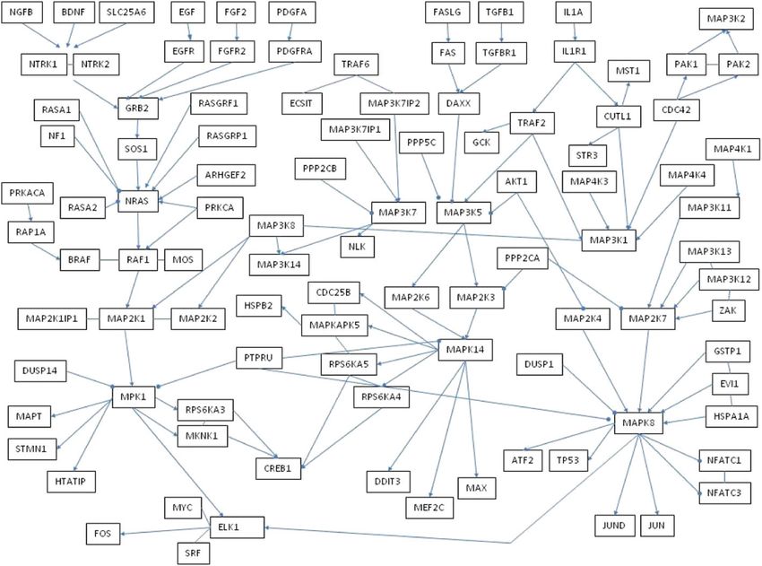
Fofana et al. Journal of Statistical Distributions and Applications   (2021) 8:9                                  Page 2 of 17

                    Introduction
                    x Gene expression data can be analyzed in a multiple testing setting as well as many
                    other statistical methods. The validity of each test depends on the underlying distribu-
                    tional assumptions of the test. A proper analysis of gene expression data requires taking
                    assumptions, usually normality, into consideration (Pounds and Fofana 2012; Pounds and
                    Rai 2009). In addition to incorporating distributional assumptions into the overall test-
                    ing, it may also be informative to incorporate any prior knowledge of association between
                    entities (Bowman and George 1995). Such associations are often recorded by graphical
                    networks (Wei and Pan 2008). Combining these different elements, besides gaining statis-
                    tical power, provides a framework through which analysis of gene expression data can be
                    improved. We propose a novel statistical approach that incorporates testing for distribu-
                    tional assumption validity with prior information provided by gene graphical network. In
                    particular, we use graphical networks to incorporate spatial dependence into the analysis
                    of gene expression data. The spatial correlation is taken into account by assuming similar
                    prior probabilities for neighboring genes.
                      We compare our approach with other methods through a series of simulations,
                    and demonstrate that hybrid-network leads to an improvement on power over other
                    approaches in most of the settings. The comparison of the different methodologies is
                    based on specificities and/or Area under the ROC Curve (AUC). The specificity of a test
                    is called the true negative rate; it is the proportion of samples that test negative using
                    the test in question that are genuinely negative. An ROC curve or a receiver operating
                    characteristic curve shows the performance of a classification model at all classification
                    thresholds. An ROC curve is constructed by reporting sensitivities, true positive rates, on
                    the y-axis and false positive rates on the x-axis.
                      The network analysis we use is the conditional autoregressive (CAR) model. CAR
                    models are commonly used to represent spatial autocorrelation in data relating to a set
                    of non-overlapping areal units. Those models are typically specified in a hierarchical
                    Bayesian framework, with inference based on Markov Chain Monte Carlo (MCMC) sim-
                    ulation. The most widely used software to fit CAR models is WinBUGS or OpenBUGS.
                    In our work, we use an R function BUGS(·) that helps run OpenBUGS inside R software.
                    Another R function, CARBayes(·), is described in Lee (2013) that can be used for Bayesian
                    spatial modeling with conditional autoregressive priors. Using CARBayes the spatial adja-
                    cency information can be specified as a neigbourhood matrix, whereas, with BUGS(·), the
                    user has to specify an adjacency matrix.

                    Material and methods
                    Network information can be represented by directed or undirected graphs. Graphs are
                    structures of discrete mathematics and have found applications in scientific disciplines
                    that consider networks of interacting elements, such as genes that interact by sharing
                    some biological resemblances. A graph consists of a set of nodes and a set of edges that
                    connect the nodes. Usually the nodes are the entities of interest. For instance, each gene
                    can be considered a node and the edges the relationships among the genes. A graph can
                    be used in a practical way by developing software to translate between representations, a
                    process sometimes referred to as “coercion”.
                      In data analysis, graphs provide a data structure for knowledge representation, for
                    example in the Gene Ontology (GO). Many studies incorporate gene network information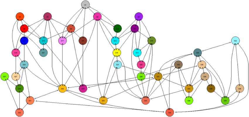
Fofana et al. Journal of Statistical Distributions and Applications    (2021) 8:9                                       Page 3 of 17

                      Fig. 1 Undirected Graphs

                    in data analysis through the GO project. Graphs provide a computational object that can
                    easily and naturally be used to reflect physical objects and relationships of interest. Graphs
                    are important to statistical methodology for exploratory data analysis. A knowledge-
                    representation graph can be juxtaposed with observed data to guide the discovery of
                    important phenomena in the data. In statistical inference, inferential statements about
                    relations between genes due to significantly frequent co-citation, or relation between gene
                    expression and protein complex can be made, (Wei and Pan 2008).
                      A graph may be directed or undirected. A directed edge is an ordered pair of end-
                    vertices that can be represented graphically as an arrow drawn between the end-vertices.
                    In such an ordered pair the first vertex is called initial vertex or tail and the second the
                    terminal vertex or head. An undirected graph disregards any sense of direction and treats
                    both head and tail identically, see Fig. 1.

                    Theory/Calculation
                    Statistical models for hybrid testing
                    Considerthe following multiple hypothesis testings

                          Hog : θ g = θ og vs H1g : θ g  = θ og , g = 1, · · · , G,                             (1)

                    with θg , a parameter for gene g, and G is the total number of genes, Hog , the null hypothe-
                    sis, and H1g is the alternative hypothesis. Suppose two mutually exclusive test procedures,
                    M1 and M2 , can be used to perform these statistical tests. When M1 is used, suppose
                    T1 = {T11 , · · · , T1G } represents the test statistics and P1 = {P11 , · · · , P1G } the corre-
                    sponding set of p-values, and suppose T2 = {T21 , · · · , T2G } and P2 = {P21 , · · · , P2G } the
                    corresponding quantities for procedure M2 .
Fofana et al. Journal of Statistical Distributions and Applications (2021) 8:9 Page 4 of 17
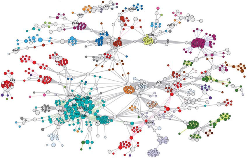
Fig. 2 Simulation Network
Suppose Ag = i is an indication that the assumption for gene g holds for procedure Mi
for testing Hog vs H1g , i = 1, 2. For testing
HogA : Ag = 1, g = 1, · · · , G, (2)
suppose Ta = {Ta1 , · · · , TaG } are the test statistics obtained from Ag with the corre-
sponding set of p-values Pa = {Pa1 , · · · , PaG }.
And then, from this method, we define an appropriate summary statistic and denote it by
P = {P1 , · · · , PG } with
P1g , if Ag = 1
Pg =
P2g , if Ag = 2
g = 1, · · · , G.
The following theorem states the distribution of Pg under the null hypothesis Hog of
Eq. (1).
Theorem Suppose there are only two mutually exclusive procedures M1 and M2 that
can be used to test the null hypothesis
H0 : θ = θ 0 . (3)
Let P1 be the p-value obtained if method M1 is used for testing the null hypothesis H0 ,
and P2 be the p-value if method M2 is used instead. Let P be defined by
P1 , if M1
P=
P2 , if M2 .
Then P is uniformly distributed under the null hypothesis H0 .
Proof First, we recall some probability theory basics. Let M1 , M2 , · · · , Mn be a partition
of a sample space , that is Mi ∩ Mj = ∅ ∀ i = j and ni Mi = . Then, for any event
E ⊂ ,
E = E ∩ ( ni Mi )
= ni (E ∩ Mi )
and then for any probability P,Fofana et al. Journal of Statistical Distributions and Applications (2021) 8:9 Page 5 of 17
n
P(E) = P E ∩ i Mi
n
P(E) = P (E ∩ Mi )
n i
= i P(E ∩ Mi ) (Law of total probability)
= ni P(E | Mi ) × P(Mi ) (Bayes’ rule).
Also, the law of total probability holds for conditional probability, that is
P(E | B) = ni P(E ∩ Mi | B), ∀ event B (Law of total probability)
n
= i P(E | Mi , B) × P(Mi | B) (Bayes’ rule).
n n
We recall that P() = P i Mi = i P(Mi ) = 1.
The question is to show that the hybrid p-value, P, follows a uniform distribution under
the null hypothesis (H0 ); that is FP (p) = P(P < p | H0 ) = p, ∀p ∈ (0, 1), with FP the
cumulative distribution function of P.
Under the null hypothesis (H0 ) of primary interest (gene is expressed, say) and under
M1 and M2 , respectively, both P1 and P2 are uniformly distributed, that is P(P1 < p |
M1 , H0 ) = p and P(P2 < p | M2 , H0 ) = p, see (Pounds and Rai 2009) for instance.
Recall that P is a random variable, since P1 and P2 are random variables. For the proof, we
consider M1 and M2 as two events. The notation | H0 means under the null hypothesis
(H0 ).
P(P < p | H0 ) = P (P < p)∩[ M1 ∪ M2 ] | H0 (since M1 and M2 form a partition)
= P (P < p) ∩ M1 | H0 + P (P < p) ∩ M2 | H0
(since M1 and M2 are mutually exclusive)(Law of total probability)
= P(P < p | M1 , H0 )P(M1 | H0 )+
P(P < p | M2 , H0 )P(M2 | H0 )
(Bayes’ rule).
= P(P1 < p | M1 , H0 )P(M1 | H0 ) + P ((P2 < p) | M2 , H0 ) P(M2 | H0 )
= pP(M1 | H0 ) + pP(M2 | H0 )
= pP(M1 | H0 ) + p(1 − P(M1 | H0 ))
= p.
Thus P is uniformly distributed under H0 .
Now, transform the p-values by
Zg = −1 1 − Pg , (4)
where is the cumulative distribution function of the standard normal distribution
N(0, 1), and Pg is the p-value corresponding to test g. The null distribution of Zg is the
standard normal under Hog of Eq. (1). Assume that under the alternative Zg ∼ N μ1 , σ12 ,
then
f (zg ) = π0 φ(zg ; 0, 1) + (1 − π0 ) φ zg ; μ1 , σ12 , (5)
where φ(·; μ1 , σ12 ) is the probability density function of N(μ1 , σ12 ), f is a density function.
Table 1 2−Group simulation specificity comparison
Sample size (ni ) T-test Wilcoxon test Hybrid-Network test
5 0.571726 0.557244 0.575314
10 0.689223 0.69797 0.716146
25 0.884244 0.918197 0.921273
50 0.9839 0.994575 0.994575Fofana et al. Journal of Statistical Distributions and Applications (2021) 8:9 Page 6 of 17
Bayesian hierarchical models for spatial data
Conditional autoregressive (CAR) models are commonly used to represent spatial auto-
correlation in data relating to a set of non-overlapping areal units. Those data are
prevalent in many fields like agriculture (Besag and Higdon 1999), and epidemiology (Lee
2011). There are three different CAR priors commonly used to model spatial autoregres-
sion. Each model is a special case of a Gaussian Markov random field (GMRF) that can be
written in a general form as
φ ∼ N 0, τ 2 Q−1 (6)
where Q is a precision matrix that controls for the spatial autocorrelation structure of
the random effects, and is based on a non-negative symmetric G × G neighborhood or
weight matrix W, W = (wkj ) where wkj = 1 if genes k and j are neighboring genes and
wkj = 0 otherwise, and φ = (φ1 , · · · , φG ), is a set of random effects. CAR priors are
commonly specified as a set of G univariate fully conditional distributions ξ(φk | φ −k )
for k = 1, · · · , G where φ −k = (φ1 , · · · , φk−1 , φk+1 , · · · , φG ), and G is the total number of
genes (Lee 2013; Lee 2011). The first CAR prior proposed by Besag et al. (1991) is as
G
j=1 wkj φj τ2
φk | φ −k ∼ N G , G . (7)
j=1 wkj j=1 wkj
The conditional expectation is the average of the random effects in neighboring genes,
while the conditional variance is inversely proportional to the number of neighbors. The
inverse proportionality of conditional variance is due to the fact that if random effects
are spatially correlated then the more neighbors a node has the more information there
is from its neighbors about the value of its random effect (subject-specific effect). This
first CAR prior is used to implement the hybrid-network methodology as in Wei and Pan
(2008). The second CAR prior proposed by Leroux et al. (1999) is given by
ρ G j=1 wkj φj τ2
φk | φ −k ∼ N G , G , (8)
ρ j=1 wkj + 1 − ρ ρ j=1 wkj + 1 − ρ
while the third CAR prior proposed by Stern and Cressie (1999) is defined by
ρ G j=1 wkj φj τ2
φk | φ −k ∼ N G , G , (9)
j=1 wkj j=1 wkj
where ρ is a spatial autocorrelation parameter, with ρ = 0 corresponding to indepen-
dence and with ρ = 1 corresponding to a strong spatial autocorrelation. A uniform prior
on the unit interval is specified for ρ, that is ρ ∼ ∪(0, 1), while the usual uniform prior
on (0, Mτ ) is assigned to τ 2 , with the default value being Mτ = 1000. The intrinsic CAR
prior by Besag et al. (1991) is obtained from the second and third CAR priors when ρ = 1,
while when ρ = 0 the difference is on the denominator in the conditional variances.
Table 2 3−Group simulation specificity comparison
Sample size (ni ) ANOVA test Kruskal-Wallis test Hybrid-Network test
5 0.579557 0.57232 0.585729
10 0.668287 0.668287 0.684932
25 0.89141 0.918197 0.929054
50 0.92437 0.9839 0.985663Fofana et al. Journal of Statistical Distributions and Applications (2021) 8:9 Page 7 of 17
Standard and spatial normal mixture model
Multipletesting is often an essential step in the analysis of high-dimensional data, such
as genomic or proteomic data. The data analysis can be based on p-values, z-scores, t-
scores, etc. These test statistics are obtained from data reduction techniques. The hybrid
p-values discussed in “Statistical models for hybrid testing” section is an example. Con-
sider for example a test statistic Z. We can assume that across hypotheses g = 1, · · · , G
the test statistic Zg follows a two-component mixture with density f as in (5). From this
two-component mixture two different types of mixture models, the standard and spatial
normal mixture models are considered. While spatial normal mixture models consider
network information in the analysis, the standard normal mixture models do not.
Standard normal mixture model
In a standard two-component mixture model, Zg has a density function f of the form
f (zg ) = π0 fo (zg ) + (1 − π0 )f1 (zg ), (10)
where π0 is the proportion of genes that are not expressed (null hypothesis), fo is the
distribution of Zg under the null hypothesis, and f1 is the distribution of Zg under the
alternative hypothesis.
Spatial normal mixture model
In a spatial normal mixture model, one defines gene-specific prior probabilities
πgs = P(Tg = s) for g = 1, · · · , G and s = 0, 1, (11)
where Tg is defined by
1 if gene g is expressed
Tg =
0 if gene g is not expressed
therefore, the marginal distribution of Zg is
f (zg ) = 1s=0 f zg | Tg = s P(Tg = s)
(12)
= πg0 fo (zg ) + πg1 f1 (zg ),
where zg is the expression value of gene g for g = 1, · · · , G, and πg1 = 1 − πg0 . It is
believed that genes on the same network, that is a group of genes with the same func-
tion, share the same prior probability of expression while different networks have possibly
varying prior probabilities. The prior probabilities πgs , based on a gene network, are
related to two latent Markov random fields xs = xgs ; g = 1, · · · , G , s = 0, 1 by a logistic
transformation:
exp(xgs )
P(Tg = s) = πgs = . (13)
exp(xg0 ) + exp(xg1 )
Each of the G-dimensional latent vectors xs is distributed according to an intrinsic
Gaussian conditional auto-regression model (ICAR) (Besag and Kooperberg 1999). The
distribution of each spatial latent variable xgs conditional on x−gs = {xks ; k = g} depends
only on its direct neighbors. To be more specific,
⎛ ⎞
1 σ 2
xgs | x−gs ∼ N ⎝ xls , cs ⎠ (14)
mg mg
l∈δgFofana et al. Journal of Statistical Distributions and Applications (2021) 8:9 Page 8 of 17
where δg is the set of indices for the neighbors of gene g, and mg is the corresponding
number of neighbors. The other model specifications are articulated in this way
(Zg | Tg = s) ∼ N μs , σs2 , (15)
g = 1, · · · , G and s = 0, 1. Network structure is summarized in a matrix format called an
adjacent matrix: Adj = (aij ), i = 1, · · · , G; j = 1, · · · , G, where
1, if i = j and genes i and j are related
aij =
0, otherwise.
Prior distributions
In a standard normal mixture model, a beta distribution is often assumed as the prior
distribution for π0 . In a spatial normal mixture model, gene-specific prior probabili-
ties are introduced. For the spatial normal mixture model, the prior probabilities for
πgs , based on a gene network, are related to two latent Markov random fields (MRFs),
as mentioned previously. From Eq. (14), we assume priors on the variance components
σcs2 ∼ inverse-gamma(0.01, 0.01), the corresponding precision σ12 has gamma(0.01, 0.01)
cs
with mean 1 and variance 100. σcs2 acts as a smoothing parameter for the spatial field
and consequently controls the degree of dependency among the prior probabilities of the
genes. The size of σcs2 determines how similar the πgs are. The smaller the σcs2 are, the more
similar the πgs .
Maximum a posterior estimation
A frequentist estimation of a standard mixture model via maximum a posterior estimation
(MAPE) is used to show the effectiveness of Bayesian estimation for mixture models.
Consider a standard mixture model, Eq. (10), with
Z ∼ N μs , σs2 (16)
Fig. 3 Comparison of AUCFofana et al. Journal of Statistical Distributions and Applications (2021) 8:9 Page 9 of 17
with θ s = μs , σs2 , s = 0, 1 and Z is a gene expression test statistic. A direct approach to
estimate π0 , π1 , θ 0 , and θ 1 is to compute the likelihood function
L(π0 , π1 , θ 0 , θ 1 ) = nk=1 G f (zgk )
n g=1 G (17)
= k=1 g=1 π0 fo (zgk , θ 0 ) + π1 f1 (zgk , θ 1 )
and the log likelihood as
n G
l(π0 , π1 , θ 0 , θ 1 ) = log[ π0 fo (zgk , θ 0 ) + π1 f1 (zgk , θ 1 ] . (18)
k=1 g=1
Obtaining MAPE’s of the parameters directly is not possible. To estimate the parame-
ters the expectation-maximization (EM) algorithm may be used. In order to use the EM
algorithm, define latent variables v = (vgk , zgk ) | k = 1, · · · , n and g = 1, · · · , G where
1, if g ∈ G1
vgk =
0, if g ∈ G0
with G0 (genes not expressed) and G1 (expressed genes) are null hypothesis and alterna-
tive groups respectively, n is the sample common to all genes. If we include latent variables
we get complete data, the observed z s and the unobserved v s. The maximum a posterior
function for the complete data is
n
G
1−vgk v
Lc (π0 , π1 , θ 0 , θ 1 | z, v) = π0 fo (zgk , θ 0 ) π1 f1 (zgk , θ 1 ) gk . (19)
k=1 g=1
Taking the log on Eq. (19) we get the log maximum a posterior function as
n G
lc (π0 , π1 , θ 0 , θ 1 | z, v) = (1 − vgk )log[ π0 fo (zgk , θ 0 )] +vgk log[ π1 f1 (zgk , θ 1 ] .
k=1 g=1
(20)
The EM algorithm can be used to obtain MAPE’s of π0 , π1 , θ 0 and θ 1 , if (z1k , z2k , · · · , zGk )
are assumed to be independent.
However, since there is a graphical network among genes, (z1k , z2k , · · · , zGk ) are not
independent. In order to take into account gene graphical network a Bayesian methodol-
ogy is used. Network analysis is brought into the analysis by generating latent variables
according to GMRFs as in Eq. (14). After assigning prior distributions to the parameters,
posterior distributions can be found using a partial Gibbs sampler and some Metropolis
Hasting algorithms. We use OpenBugs software to get the MAPE’s of π0 , π1 , θ 0 , and θ 1 .
Statistical inference
The decision rule and acceptance of null hypotheses is based on probabilities from poste-
rior distributions. For each gene g, the point estimate of p(H0g | Data) is computed and
compared to a threshold τ , for g = 1, · · · G. H0g is rejected when p̂(H0g | Data), the point
estimate, of p(H0g | Data) is less than a threshold τ .
The p-values pg obtained from the hybrid method are transformed, and the transformed
statistics zg = −1 (1 − pg ) are used, with −1 the standard normal quantile func-
tion. Through Bayesian modeling, network information is added to the analysis. With the
Bayesian inference these posterior estimates are π̂g0 = p̂(H0g | Data). Inferences for the
Bayesian hierarchical models are obtained using MCMC simulations, with a combinationFofana et al. Journal of Statistical Distributions and Applications (2021) 8:9 Page 10 of 17
Fig. 4 Gene Graphical Network
of Gibbs sampling and Metropolis steps. Gibbs sampling is used to do MCMC simulation
for fully conditional posteriors with closed forms. For those that are not in closed forms
the Metropolis-Hasting algorithm is used.
Results
Simulations
To compare the hybrid-network method with other methods, we conducted simulation
studies designed to mimic real data analysis. We conducted standard two-group compari-
son studies (treatment vs control), k-group (k > 2) comparison (ANOVA), and regression
analysis. The k-group comparison is directly applicable to a genomic study comparing
human ependymoma, a brain tumor that occurs in three distinct anatomic regions: Pos-
terior Fossa (PF), Spine (SP), and Supratentorial (ST). Regression analysis is often useful
to determine whether, for example, gene expression levels are related to a particular
covariate such as DNA synthesis rate (INHIBO).
For each of the three types of analyses conducted in the simulation studies, two differ-
ent tests can be used. The first one requires the normality assumption while the second
may be appropriate when the normality assumption does not hold. For the two-group
comparison the hybrid-network method chooses between the standard t-test for normally
distributed data and the Wilcoxon test when the normality assumption fails. For k-group
(k > 2) comparison, the hybrid-network method chooses between the standard ANOVA
test and the Kruskal-Wallis test. For the regression analysis, the Pearson test for linear
dependency is chosen when the normal assumption holds and the Spearman test if the
normality assumption does not hold.Fofana et al. Journal of Statistical Distributions and Applications (2021) 8:9 Page 11 of 17
In Eq. (12), we use π̂g0 , the estimate of πg0 . And, the decision rule consists of rejecting
the null hypothesis, Hg0 , for gene g, if π̂g0 is less than a threshold, τ . The conclusion is that
the corresponding gene g is expressed. For cancer data analysis, for instance, if a gene is
expressed, health researchers will target that gene in finding cure.
The comparison of the different methodologies is mainly based on specificities (not to
reject the null hypotheses when they are true, we call them sometimes true negatives). We
could provide both specificities and sensitivities (reject the null hypotheses when they are
not true, we call them sometimes true positives); but we have decided to compute only
specificities because the simulations are computationally intensive.
K-group comparison study
In a group comparison study, gene expression data can be modeled as:
Ygij = μg + τgi + gij , (21)
where Ygij is the expression level for gene g of the jth individual in the ith group,
g = 1, · · · , G, i = 1, · · · , k; j = 1, · · · ni ,
k is the number of groups, ni is the sample size of group i, and
gij ∼ N(0, 1) or gij ∼ t(ν), or gij ∼ another distribution.
A 2-group comparison (k = 2), interest is in statistical tests of the form
Hg0 : μg1 = μg2 vs HgA : μg1 = μg2 , (22)
g = 1, · · · , G. Some gene expression levels may be normally distributed while others are
not normally distributed. In the two-group comparison study, two tests are often used.
The t-test is used when the normality assumption holds and the Wilcoxon test, a non
parametric test, is often used when the normality assumption does not hold. For each gene
g, a t-test, a Wilcoxon-Mann-Whitney rank sum test, and a Shapiro-Wilk test statistics are
computed. Diagnoses for adequacy of the t-test statistics are made through residuals. We
compute the residuals from the t-test statistic. We define the residuals on observation, j,
in treatment, i, for gene, g, as
egij = Ygij − Ŷgij (23)
where Ŷgij is an estimate of the corresponding observation Ygij obtained as follows:
Ŷgij = μ̂g + τ̂gi
= Ȳg·· + Ȳgi· − Ȳg·· (24)
= Ȳgi· .
If the model is adequate, residuals should be structure-less; that is, they should contain
no obvious patterns. Through an analysis of residuals, many types of model inadequacies
and violations of the underlying assumptions can be discovered. We use the residuals to
check for normality. A probit plot of residuals is an extremely useful procedure to test for
normality. If the underlying error distribution is normal, this plot will resemble a straight
line. Also outliers can be detected through residuals. Outliers show up on probability
plots as being very different from the main body of the data. Plotting the residuals in time
order of data collection is helpful in detecting correlation between the residuals. This is
useful for checking independence assumptions on the errors.Fofana et al. Journal of Statistical Distributions and Applications (2021) 8:9 Page 12 of 17
To compare the hybrid-network method with other methods, we perform a simulation
study. In this setup, there are two groups of sample sizes varying from 5, 10, 25, and 50.
The number of gene expressions having a normal distribution, N(μ, 1), is 30. For these
gene expressions, μ = 0 for the null hypothesis and μ = 1 for the alternative. The remain-
ing gene expressions have log-normal distribution, log-normal (μ, 1), with μ = 0 in some
cases and μ = 1 in other cases. And a graphical network, Fig. 2, is built among genes with
212 number of edges. We translate this graphical network into an adjacent matrix.
The results are presented in Table 1, they show that hybrid-network procedure dom-
inates the other methodologies in most of the settings, since the hybrid-network test
specificities are higher than the specificities of the other methods. When the sample
size is equal to 5, for instance, the specificity corresponding to the t-test is 0.571726,
the specificity corresponding to the Wilcoxon test is 0.557244, and the specificity for the
hybrid-network test is 0.575314.
Hybrid ANOVA-Kruskal Wallis study
In a k-group comparison study, a statistical model can be written as Eq. (21). For the
model (21), μg is a parameter common to all treatments for gene g called the overall mean,
and τgi is a parameter unique to the ith treatment for gene g called the ith treatment effect.
Consider the following multiple hypothesis tests
Hg0 : μg1 = μg2 = · · · = μgk vs HgA : μgi = μgl for at least one pair (i, l) (25)
or equivalently, by using the effects models
Hg0 : τg1 = τg2 = · · · = τgk = 0 vs HgA : τgi = 0 for at least one i. (26)
The hypotheses may be tested using an ANOVA test or the Kruskal-Wallis depending on
the normality assumption. If the normality assumption is valid, the ANOVA test is more
powerful than the Kruskal-Wallis; and the latter may be more powerful when the normal-
ity assumption does not hold. The proposed methodology, hybrid-network, combines a
test of assumptions and graphical network information into the analysis. For each gene g,
an ANOVA p-value, pag , a Kruskal-Wallis p-value, Pgw , and a Shapiro-Wilk p-value, Pgs are
computed. We define a hybrid p-value, Pgh , as
Pga , if Pgs ≥ α
Pgh =
Pgk , if Pgs < α,
for g = 1, · · · , G where α is a given threshold. The hybrid p-value Pgh is transformed into
a hybrid z-statistic, zgh , as follows:
zgh = −1 1 − Pgh . (27)
We use zgh to build a CAR model from the given network with the marginal distribution
of zgh given by
f zgh = πg0 fo zgh + πg1 f1 zgh , (28)
where zgh is the expression value for gene g, g = 1, · · · , G.Fofana et al. Journal of Statistical Distributions and Applications (2021) 8:9 Page 13 of 17
Table 3 Human ependymoma microarray data
Genes Gr1 Gr1 ··· Gr2 Gr2 ···
AKT1 12.48167 11.75317 ··· 10.95536 11.51737 ···
ARHGEF2 14.99632 13.81004 ··· 13.45263 14.02982 ···
ATF2 12.93096 13.14289 ··· 13.44182 12.72238 ···
BDNF 3.392317 4.542258 ··· 4.716991 5.738768 ···
BRAF 9.111918 10.3433 ··· 10.07682 9.107217 ···
CDC25B 10.33114 11.04207 ··· 11.7139 11.76408 ···
.. .. .. .. .. .. ..
. . . . . . .
This shows the human ependymoma expression data: genes as gene annotation, groups (Gr1 and Gr2) as sample annotation and
real values as gene expression levels.
The prior probabilities πgs , based on a gene network, are related to two latent Markov
random fields xs = {xgs ; g = 1, · · · , G}, s = 0, 1 by a logistic transformation:
exp(xgs )
P(Tg = s) = πgs = . (29)
exp(xg0 ) + exp(xg1 )
The distribution of each spatial latent variable xgs conditional on x−gs = {xks ; k = g}
depends only on its direct neighbors. The proposed CAR prior distribution from (Besag
and Kooperberg 1999) is used as
⎛ ⎞
1 σ 2
xgs | x−gs ∼ N ⎝ xls , cs ⎠ , (30)
mg mg
l∈δg
where δg is the set of indices for the neighbors of gene g, and mg is the corresponding
number of neighbors.
The hybrid-network methodology, through a series of simulations, is compared to other
methods. The setup of these simulations consists of three groups of sample size varying
from 5, 10, 25, and 50. The number of genes with the normal distribution N(μ, 1), μ = 0
for the null hypothesis and μ = 1 for the alternative, is 30. The number of genes with the
log-normal distribution, log-normal(μ, 1), with μ = 0 in some cases and μ = 1 in other
cases, is 7 and the number of genes with the Cauchy distribution, Cauchy(θ, 1), with θ = 0
in some cases and θ = 1 in other cases, is 7. A graphical network is built among genes
with 212 edges. We present the simulations results in Table 2. They show that hybrid-
network procedure dominates other procedures in most of the cases. When the sample
size is 25, for instance, the specificities from the ANOVA test, the Kruskal Wallis and the
hybrid-network test are 0.89141, 0.918197, and 0.929054, respectively.
Regression analysis
In microarray regression analysis, a statistical model can be written as
Ygj = βg0 + Xgj βg1 + gj (31)
where Ygj is the gene expression level for the g th gene in the jth individual with
g = 1, · · · , G, j = 1, · · · , n
and some
gj ∼ N(0, 1) or gj ∼ t(ν), or gj ∼ another distribution.Fofana et al. Journal of Statistical Distributions and Applications (2021) 8:9 Page 14 of 17
Fig. 5 Tumor Data 2-Group Comparison
The question is whether a response variable and a covariate are correlated. To test for
correlation between gene expression with a covariate such as a phenotype, the analysis can
be based on Pearson test p-values (Pp ), and on Spearman test p-values (Psp ). We can use
Shapiro-Wilk p-values (Ps ) to test for the normality assumptions. Consider, the regression
analysis in matrix format
Y g = Xg β g + g (32)
where
⎡ ⎤ ⎡ ⎤ ⎡ ⎤
Yg1 1 Xg1 g1
⎢Y ⎥ ⎢1 X ⎥
⎢ ⎥
⎢ g2 ⎥ ⎢ g2 ⎥ β ⎢ g2 ⎥
Yg = ⎢ ⎥ ⎢ ⎥ ⎢ ⎥
g0
⎢ .. ⎥ ; X g = ⎢ .. .. ⎥ g; β = ; g = ⎢ .. ⎥ . (33)
⎣ . ⎦ ⎣. . ⎦ βg1 ⎣ . ⎦
Ygn 1 Xgn gn
We denote the least squares estimators of β g as bg
−1
bg = Xg Xg Xg Y g . (34)Fofana et al. Journal of Statistical Distributions and Applications (2021) 8:9 Page 15 of 17
Let the vector of the fitted values Ŷgi be denoted as Ŷg , and the vector of the residual terms
egi = Ygi − Ŷgi be as eg . The fitted values are represented by
Ŷg = Xg bg (35)
and the residuals by
eg = Yg − Ŷg . (36)
p sp
For each gene g, compute its Pearson p-value, Pg , compute its Spearman p-value, Pg ,
and from the residuals from Pearson test, a Shapiro-Wilk test of normality is performed,
and for each gene g a p-value, Pgs , is calculated. Finally, a hybrid p-value, Pgh is computed as
p
Pg , if Pgs ≥ α
Pgh = sp
Pg , if Pgs < α
where α is a given threshold.
Each hybrid p-value, Pgh , is transformed into a hybrid z-statistic, zgh , as follows:
zgh = −1 1 − Pgh . (37)
Using zgh , the marginal distribution of zgh is given as
f (zgh ) = πg0 fo zgh + πg1 f1 zgh , (38)
where zgh is the expression value of gene, g, g = 1, · · · , G.
We compare the hybrid-network with the other procedures through a simulation setup.
The setup consists of a sample size of 25. The number of genes with the normal distri-
bution, N(μ, 1), is 30, μ = 0 for the null hypothesis and μ = 1 for the alternative, and
the number of genes with the log-normal distribution, log-normal(μ, 1), with μ = 0 in
some cases and μ = 1 in other cases, is 14. We vary the cutoff point, τ , as in Wei and
Pan (2008). And a graphical network is built among genes with 212 number of neighbors.
The results of the analysis are presented in Fig. 3. In order to compare the hybrid-testing
with other methods, we use AUCs to judge the performance of the proposed method. A
greater AUC corresponds to a better methodology. They show that the hybrid-network
performs better than the other competing procedures.
Application to human ependymoma microarray
We compare the hybrid-network procedure with the t-test and the Wilcoxon test using
human ependymoma data. The data consists of gene expression levels, gene annotation,
sample annotation, and a gene graphical network. Figure 4 illustrates a graphical network
of the genes under consideration, and Table 3 is a subset of the human ependymoma
expression data. In this analysis, there are two groups, the sample sizes are n1 = 37 for
group1, n2 = 42 for group2, with the total number of genes of 102, and the number of
edges is 196. The data and the R codes can be requested from the corresponding author.
Using Shapiro-Wilk p-values, it appears that some of the expression data are normally
distributed and the others are not, with Shapiro-Wilk test p-values less than α = 5%
for some genes. Figure 5 shows histograms of p-values from the t-test, p-values from the
rank sum test, and p-values based on the Shapiro-Wilk test of normality, respectively.
The last graph of Fig. 5 presents the plot of the p-values from the t-test with respect toFofana et al. Journal of Statistical Distributions and Applications (2021) 8:9 Page 16 of 17
Fig. 6 Tumor Data: Analysis Results
the corresponding p-values from the rank sum test. Using the t-test when the normal-
ity assumption is assumed, and the Wilcoxon test otherwise. We apply the hybrid-testing
procedure to analyze the data. We incorporate a graphical network to accommodate inter-
actions between genes, as these have been noted to play a crucial role in cell functions
(Shojaie and Michailidis 2009).
In order to compare the hybrid-network procedure with the other procedures, we
report results for the first six genes. We use box plots as visual methods of comparing
groups. Under each Box plot, we report the results, π̂·0 , with t representing the t-test
statistic , rs for Wilcoxon test statistic, and hybN for hybrid-network statistic. We also
present the p-values from Shapiro Wilk test (Shp) under each box plot. The results are
reported on Fig. 6.
With a cutoff point of τ = 0.1, (τ is is a classification threshold, it is like, say α, the
level of significance, see Wei and Pan (2008)), all the three methods find that genes AKT1,
ATF2, and CDC25B are not expressed. Only the hybrid-network test finds that the other
three genes, ARHGEF2, BDNF and BRAF are expressed. This finding is in accordance
with the box plot results. The gene selection is based on R head(·) function, that selects
the 6-first results. By doing so, we have tried to avoid criticism of biasness in selecting
genes to analyze. First, we sort the genes and then pick the 6-first genes for comparing
the different methodologies.Fofana et al. Journal of Statistical Distributions and Applications (2021) 8:9 Page 17 of 17
Discussion and conclusion
To the best of our knowledge the Hybrid-Network procedure is the very first one that
considers assumptions and a graphical network into the analysis of gene expression data.
It has a broad variety of applications and entails layers of complexities.
In simulations and in real data analysis, we show that the hybrid-Network proce-
dures perform well. Hybrid-network procedures can be applied to group comparison
analysis and to regression analysis. In the near future we are implementing a Hybrid-
Network routine that will help researchers analyze gene expressions data in a better and
proper manner. In our future research, we plan to apply this method to next generation
sequencing data.
Abbreviations
AUC: Area under the ROC curve; ROC: Receiver operating characteristic; GMRF: Gaussian Markov random field
Acknowledgments
This version is presented at the Joint of Statistical Meeting, JSM (The American Statistical Association, Chicago, IL 2016)
and is accepted on JSM Proceedings. The authors are highly indebted to participants at this conference for their valuable
comments.
Authors’ contributions
DF: literature search, model design, simulation, coding, data analysis, data interpretation, writing, critical revision. EOG:
model design, writing, critical revision. DB: writing, critical revision, data acquisition. All authors have read and approved
the final manuscript.
Funding
The International Conference on Statistical Distributions and Applications (ICOSDA).
Availability of data and materials
Data and coding are available upon request from the corresponding author.
Declarations
Competing interests
The authors declare that they have no competing interests
Author details
1 University of Texas Rio Grande Valley, Edinburg, TX 78539, USA. 2 University of Memphis, Memphis, TN 38152, USA.
Received: 28 July 2020 Accepted: 25 May 2021
References
Besag, J., Higdon, D.: Bayesian Analysis of Agricultural Field Experients. J. R. Stat. Soc. Ser. B. 61, 691–746 (1999)
Besag, J., Kooperberg, C.: On conditional and intrinsic autoregressions. Biometrika. 82, 733–746 (1999)
Besag, J., York, J., Mollié, A.: Bayesian Image Restoration with Two Applications in Spatial Statistics. Ann. Inst. Stat. Math.
43, 1–59 (1991)
Bowman, D., George, E. O.: Saturated Model for Analyzing Exchangeable Binary Data: Applications to Clinical and
Developmental Toxicity Studies. J. Am. Stat. Assoc. 90, 431 (1995)
Lee, D.: A Comparison of Conditional Autoregressive Models Used in Bayesian Disease Mapping. Spat. Spatiotemporal
Epidemiol. 2, 79–89 (2011)
Lee, D.: CARBayes: An R package for Bayesian Spatial Model with Conditional Autoregressive Priors. J. Stat. Softw. 55, 13
(2013)
Leroux, B., Lei, X, Breslow, N.: Estimation of Disease Rates in Small Areas: A New Mixed Model for Spatial Dependence. In:
Halloran, M. E., Berry, D. (eds.) Statistical Models in Epidemiology, the Environment, and Clinical Trials, pp. 135–178.
Springer, New York, (1999)
Pounds, S., Fofana, D.: Hybrid Multiple Testing (2012). http://www.bioconductor.org/packages/2.12/bioc/html/
HybridMTest.html. [accessed 12.17.12]
Pounds, S., Rai, S. N.: Assumption adequacy averaging as a concept to develop more robust methods for differential gene
expression analysis. Comput. Stat. Data Anal. 53, 1604-1612 (2009)
Shojaie, A., Michailidis, G.: Analysis of Gene Sets Based on the Underlying Regulatory Network. J. Comput. Biol. 16,
407–426 (2009)
Stern, H., Cressie, N.: Inference for extremes in disease mapping. In: Lawson, A., Biggeri, A., Boehning, D., Lesaffre, E., Viel,
J.-E., Bertollini, R. (eds.) Disease Mapping and Risk Assessment for Public Health, pp. 63–84. Wiley, Chichester, (1999)
Wei, P., Pan, W.: Incorporating Gene Networks into Statistical Tests for Genomic Data via a Spatially Correlated Mixture
Model. Bioinformatics. 24, 404–411 (2008)
Publisher’s Note
Springer Nature remains neutral with regard to jurisdictional claims in published maps and institutional affiliations.You can also read