Comparing decision mining approaches with regard to the meaningfulness of their results
←
→
Page content transcription
If your browser does not render page correctly, please read the page content below
Comparing decision mining approaches with
                                                 regard to the meaningfulness of their results
arXiv:2109.07335v1 [cs.LG] 15 Sep 2021

                                                          Beate Scheibel1 and Stefanie Rinderle-Ma2
                                             1
                                              Research Group Workflow Systems and Technology, Faculty of
                                                        Computer Science, University of Vienna,
                                                               beate.scheibel@univie.ac.at
                                         2
                                             Chair of Information Systems and Business Process Management
                                                               Department of Informatics
                                                        Technical University of Munich, Germany
                                                              stefanie.rinderle-ma@tum.de

                                                                                 Abstract
                                                     Decisions and the underlying rules are indispensable for driving process
                                                 execution during runtime, i.e., for routing process instances at alternative
                                                 branches based on the values of process data. Decision rules can comprise
                                                 unary data conditions, e.g., age > 40, binary data conditions where the
                                                 relation between two or more variables is relevant, e.g. temperature1 <
                                                 temperature2, and more complex conditions that refer to, for example,
                                                 parts of a medical image. Decision discovery aims at automatically de-
                                                 riving decision rules from process event logs. Existing approaches focus
                                                 on the discovery of unary, or in some instances binary data conditions.
                                                 The discovered decision rules are usually evaluated using accuracy, but
                                                 not with regards to their semantics and meaningfulness, although this is
                                                 crucial for validation and the subsequent implementation/adaptation of
                                                 the decision rules. Hence, this paper compares three decision mining ap-
                                                 proaches, i.e., two existing ones and one newly described approach, with
                                                 respect to the meaningfulness of their results. For comparison, we use one
                                                 synthetic data set for a realistic manufacturing case and the two real-world
                                                 BPIC 2017/2020 logs. The discovered rules are discussed with regards to
                                                 their semantics and meaningfulness.

                                         1       Introduction
                                         Process mining enables process discovery, conformance checking, and process
                                         enhancement [1]. One important aspect of process discovery is the derivation of
                                         decision points and the corresponding decision rules based on event logs [2]. The
                                         discovered decision rules are usually of the form v(ariable) op(erator) c(onstant),

                                                                                      1
i.e., a variable compared to a constant value (referred to as unary data condi-
tion), e.g., temperature below 50°. However, real-world processes often include
more complex decision rules [3]. Then, restricting discovery to unary conditions
can lead to semantically incorrect decision rules that perform well because of
overfitting, but do not appropriately depict the underlying decision logic. The
first step towards decision rules reflecting real-world needs is to consider binary
data conditions. These conditions involve two or more variables that are in a
specific relation to each other, e.g., t1 < t2 where t1 and t2 are variables and their
values are written during process runtime. Approaches such as BranchMiner [4]
enable the discovery of binary data conditions. However, again the focus is on
accuracy of the results; their semantics is not considered despite the increased
complexity of the rules.
Considering the semantics and meaningfulness of decision mining results is
especially important with respect to transparency and explainability which are
requirements for process mining [5]. Another challenge is validity. A distinction
between internal and external validity is made, where internal validity can be
loosely translated to the accuracy, whereas external validity refers to whether
the result can be generalized [5]. This translates to decision mining as well.
The discovered decision rules should be accurate, generalizable as well as trans-
parent in the sense that they depict the underlying logic. Transparency and
explainability are current challenges for machine learning in general [6], and
for decision mining in particular. Decision rules should be accurate as well as
contain meaningful rules. A first step is the ability to discover more complex
decision rules. However, this might also lead to an increased number of dis-
covered rules, which in turn amplifies the need to check for meaningfulness in
addition to accuracy.
This paper compares three decision mining approaches that enable the dis-
covery of unary and binary data conditions with respect to the semantics and
meaningfulness of the results. The first approach features a basic decision tree
implementation. The second approach is BranchMiner (BM) [4] which is avail-
able as a compiled tool without source code or detailed documentation. There-
fore, a third approach – the Extended Decision Tree (EDT) – is provided. It
builds upon the concepts of the basic tree implementation and integrates ideas
from [4] in order to enable dynamic testing and ensure transparency and com-
prehensibility of the rules. This approach is currently restricted to binary data
conditions with comparison operators, which is sufficient for the purposes of this
paper. The three approaches are compared based on two real life datasets and
one synthetic dataset. Based on the observations from the comparison we pro-
vide recommendations for the interpretation and validation of decision mining
results.
Section 2 presents a running example from the manufacturing domain. The
decision mining approaches to be compared will be described in Sect. 3. The
results are described in Sect. 4 and analyzed in Sect. 5. In Sect. 6 the related
work is discussed and Sect. 7 provides a conclusion.
22 Running Example: Measuring Process in Man-
ufacturing
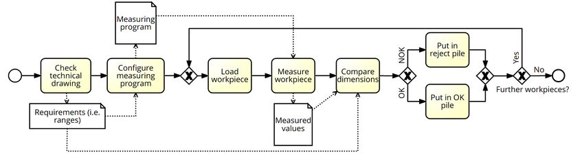
This section describes a use case from the manufacturing domain to illustrate
the challenges described in Sect. 1. In the manufacturing domain producing
workpieces and checking their quality is a core task. Workpieces are manu-
factured manually or using different machines and subsequently checked if they
adhere to the conditions (nominal value and tolerances) specified in the technical
drawing or CAD model. Measuring can be done manually or using a coordinate
measuring machine. If a measuring machine is used, the measuring program
specifies which features have to be measured for a particular workpiece. This
program has to be configured manually and is based on the technical drawing.
After the workpiece is measured, the measured values have to be checked to
make sure they adhere to the specified conditions. Then it is either placed on
the scrap pile or on a tray for further use and the process can start again. If the
measuring is done manually, some measuring tool, e.g., a calliper will be used.
The rest of the process is performed the same way. The corresponding process
model is depicted in Fig. 1.
During runtime the events reflecting the process execution are stored in a
process event log. Listing 1 shows an excerpt of a process event log for the
process model in Fig. 1. The uuid identifies the trace of a particular process
instance. The logged events reflect the execution of process tasks Prepare
attribute list and Measure workpiece with their timestamps and associated
data elements.
Figure 1: BPMN model of measuring process (modeled using Signavio© ).
Listing 1: Example log in XES format
1
2
3
4 < s t r i n g key =’ c o n c e p t : name ’
5 v a l u e =’Check t e c h n i c a l drawing ’/ >
6 < s t r i n g key =’ r a n g e s ’
7 value = ’[[20 ,25] ,[10 ,15] ,[30 ,35]] ’/ >
8
10
311 ...
12
13 < s t r i n g key =’ c o n c e p t : name ’
14 v a l u e =’ Measure w o r k p i e c e ’/ >
15 < s t r i n g key =’ m e a s u r e d v a l u e s ’
16 value = ’[24 ,12 ,31] ’/ >
17
19
20 ...
21
This process includes one decision point i.e., Dimensions in tolerance?,
which can be answered by ’Yes’ or ’No’ and the respective paths lead to either
Put in OK Pile or Put in NOK Pile. However, the underlying decision rule
is more complex (i.e., ’all measured features have to be in the specified toler-
ance zone’) and can only be obtained by discussing the process with a domain
expert. When performing this process manually, the decision is made by the
employee, who documents the measured values either digitally or on a piece of
paper. When automating the entire process, the attribute list, the list of
all essential features with the respective tolerances is stored digitally. When
the feature is measured, it can be automatically checked if it lies within the
tolerance range. This can be hard-coded as part of the process. However, it
is more challenging to automatically discover the underlying decision rule from
the event log. Table 1 can be obtained by merging the event data from one
trace into one row. It shows the identifier (the uuid), the tolerance ranges, the
measured values (abbreviated as ’meas’ in the following), as well as the result,
i.e., if the workpiece was specified as ’OK’ or ’NOK’. All list values have to be
split up into single values, in order to be used as input for the three decision
mining approaches.
Table 1: Data for running example 1.
uuid ranges meas result
0001 [(20,25),(10,15),(30,35)] [24,12,31] OK
0002 [(20,25),(10,15),(30,35)] [23,13,33] OK
0003 [(20,25),(10,15),(30,35)] [24,10,37] NOK
3 Discovering Decision Rules with Extended Data
Conditions
In general, algorithms for decision mining have to fulfill a major requirement:
the resulting decision rules have to be human readable. Therefore decision trees
are typically used for decision mining instead of black-box approaches such as
neural networks [2]. In the following, we illustrate the challenges of the basic
decision mining approach based on the running example (cf. Sect. 2), before
the BranchMiner [4] is described, and the Extended Decision Tree is introduced.
4meas0 > 21
false true
NOK meas1 < 19
NOK meas2 > 31
NOK meas2 < 69
NOK meas1 > 9
NOK meas0 < 79
NOK OK
Figure 2: Decision tree generated by basic approach.
3.1 Basic Decision Tree - BDT
Most approaches for discovering decision rules use decision trees. Well-known
algorithms include CART [7] and C4.5 [8]. Decisions are treated as a classifica-
tion problem. In the running example, the decision tree can be used to classify
a certain workpiece in ’OK’ or ’NOK’. The possible input formats include nu-
merical data and, depending on the implementation, categorical data. For the
running example, a CART implementation [9] generates the decision tree in Fig.
2, after the lists have been transformed into single valued variables. The classifi-
cation uses unary data conditions, as current decision tree implementations are
not able to discover binary data conditions. The basic approach works in many
cases and can achieve high accuracy. However, valuable semantic information
is lost in the process as we do not know the exact ranges and the underlying
relations which can lead to misleading rules and lower accuracy if the input data
changes. For example, the learning set could contain only a slight variation in
values. Thus the learned conditions contain smaller ranges than stated in the
drawing. This is the case in the running example, as well. If the conditions con-
tained in Fig. 2 are aggregated, the tolerance ranges are (22,78),(10,18),(32,69)
instead of the ranges specified in the drawing: (20,80),(10,20),(30,70). Here, the
discovered rule contains no semantic information and is slightly inaccurate.
3.2 BranchMiner - BM
BranchMiner [4] uses Daikon [10], a tool for discovering invariants in Software,
to detect invariants in event logs. Invariants refer to data conditions that are
true at one point in the process, e.g., before Event E takes place Variable v
has to have a specific value. It is able to discover unary as well as binary data
conditions and even linear relationships e.g. v1 ∗ 10 < v2. Binary conditions
are discovered using latent variables. Latent variables are additional variables
that are generated by combining all variables with each other using arithmetic
5Table 2: Running example with latent variables.
range1 range1 meas2
uuid range1 range5 meas0 meas2 ... >= >=column has to be defined. Numeric variables are used as input variables. As for
BM, latent variables enable the discovery of binary conditions. Latent variables
are generated by taking two variables and comparing them using an operator
⊗, with ⊗ ∈ {, ≤, ≥, 6=, =}. The resulting logical value is stored in a new
variable.
This is done for all variables and all comparison operators. The result for the
running example can be partially seen in Tab. 2. The data element ranges from
Tab. 1 was split into singular values (range0-range5), similar measured values
was split into meas0-meas2, this was also done for BDT. Three latent variables
are shown, i.e., range1>=range5, range>=meas0 and meas2discovered decision rule, and then compared to the actual result to check if the
instance was correctly classified.
In addition to accuracy, the recall and precision value for the discovered
rules are calculated, based on the definition by [13]. To calculate these values,
a ground truth has to be known, which refers to the conditions that are part
of the actual underlying decision rule. As the ground truth is only defined for
the running example, the other rules are estimated, based on the information
available.
Recall refers to the ratio of discovered relevant conditions to the number of
conditions in the ground truth. ’Relevant’ in this context means conditions that
are also part of the ground truth decision rule.
T otal number of discovered relevant conditions
Recall :=
T otal number of ground truth conditions
Precision refers to the ratio of discovered relevant conditions to the number of
all discovered conditions.
T otal number of discovered relevant conditions
P recision :=
T otal number of ground truth conditions
The recall value can be used to evaluate if all underlying conditions have been
discovered. Precision can be used to evaluate the complexity and comprehen-
sibility of the discovered rules, i.e., if precision is 1, only relevant conditions
are extracted. It is necessary to find a balance between these two values, as it
is desirable to discover as many underlying conditions as possible without too
many meaningless conditions which would add complexity and therefore lead
to less comprehensible rules. Therefore, the F1 measure [14] can be used as it
combines these recall and precision into one metric.
precision ∗ recall
F1 := 2 ∗
precision + recall
The closer to 1, the higher are recall and precision and therefore the better is the
ground truth represented by the discovered rule. Inversely, the closer to 0 this
value is, the worse it represents the underlying rule. The calculation of the F1
measure is only possible if precision and recall are not zero, as otherwise an error
will occur, due to division by 0. The comparison of the discovered conditions
with the conditions contained in the ground truth rule is done manually.
4.1 Synthetic Data Set (Running Example)
This data set consists of synthetic data for 2000 workpieces based on the process
model depicted in Fig. 1. As result variable, we define the column ’res’ that
specifies if the workpiece is ’OK’ or ’NOK’(1 / Branch1 → OK, 0 → NOK).
The remaining variables are used as input columns. The ground truth is known
for this case, as it was used to simulate the data and can be seen in Ground
Truth, Synthetic.
8Ground Truth, Synthetic:
meas0 >= range0 AND meas0 = range2 AND
meas1 = range4 AND meas2 9.5 implies that 9.6 is already in the valid range which could lead
to false results. As this approach is not able to correctly detect the binary
conditions, recall and precision are 0 and therefore the F1 measure is undefined.
Rule BDT, Synthetic:
WHEN meas1 > 9.5 AND meas1 meas1 = f alse AND meas1 =
meas2 = true AND meas0 < range0 = f alse AND range1 >= meas0 = true AND
range4 > meas2 = f alse THEN Y = 1,
Accuracy: 100%,
Recall: 1, Precision: 1, F1 : 1
94.2 BPIC 2017 The BPIC 2017 data set2 captures a loan application process. The result is defined as the decision if the loan conditions were accepted (1/Branch1 → accepted, 0 → not accepted). As input all numerical variables are used as no prior information is available which variables are relevant for the decision rules. The ground truth decision rule is estimated, and will reflect the underlying rule only partly. However, we assume that that the offered amount being at least the same as the requested amount is a precondition for acceptance. Ground Truth, BPIC2017: Of f eredAmount >= RequestedAmount For BDT, the accuracy is 72% and the conditions are meaningless with recall and precision values of 0 and seem overly complex. For example the variable N umberOf T erms is used several times and is unlikely to have an impact on the decision. Rule BDT, BPIC2017: WHEN CreditScore 47.5 AND Selected
N umberOf T erms. 3 The accuracy is 73% and slightly exceeds the ones of BDT
and BM for BPIC2017. The F1 measure is 0.25, due to a recall value of 1 and
the precision value of 0.14. However, the value of 1 as recall value is most likely
an overestimation as only one underlying condition was defined, whereas the
true ground truth probably contains more conditions.

    Rule EDT, BPIC2017:
    WHEN N umberOf T erms
Rule BM, BPIC2020:
WHEN !(OverspentAmount > RequestedBudget) THEN Branch1,
Accuracy: 84.5%,
Recall: 0, Precision: 0, F1 : Undefined
The accuracy of 83% for EDT is below the accuracy values obtained for BDT
and BM on BPIC2020. However, the discovered rule Rule EDT, BPIC2020
seems more meaningful: it states that as soon as the requested budget is smaller
than the totally declared one, i.e., the money that was spent, overspent is true,
leading to an overall F1 value of 1. The resulting decision tree can be seen in
Fig. 4
Rule EDT, BPIC2020:
WHEN RequestedBudget < T otalDeclared = true THEN Y = 1,
Accuracy: 83%,
Recall: 1, Precision: 1, F1 : 1
RequestedBuget < T otalDeclared
false true
Not Overspent Overspent
Figure 4: Decision tree generated by EDT for BPI20.
5 Discussion
The ground truth is only known for the running example. The results for the
other two datasets are interpreted using the available description. All results
can be seen in Tab. 3.
For the running example, BDT extracts unary conditions similar to the
dimension ranges, leading to an accuracy of 100%. However, the accuracy can
drop if the ranges change or if the measured values lie closer to the ends of the
ranges. BM detects unary and binary conditions, with an accuracy of 98.7%.
The discovered rule partly reflects the underlying rule. EDT discovered all
underlying conditions and achieves an accuracy of 100%. It is interesting that
EDT achieves a more meaningful result than BM, even though it is based on
BM. The more meaningful results also reflects in a higher F1 value, which is 1
for EDT and 0.16 for BM.
For the BPIC17, the accuracy for all approaches is around 70%. BDT leads
to an extensive rule, however the discovered conditions seem meaningless. BM
detects a single binary condition, which also contains no semantic meaningful-
ness. EDT generates an extensive rule. However, only one of the discovered
conditions is meaningful. With this exception, none of the approaches was able
12Table 3: Results.
Rule Accuracy Recall Precision F1 Measure
BDT, Synthetic 100% 0 0 U*
BM, Synthetic 98% 0.16 0.16 0.16
EDT, Synthetic 100% 1 1 1
BDT, BPIC2017 72% 0 0 U
BM, BPIC2017 70% 0 0 U
EDT, BPIC2017 73% 1 0.14 0.25
BDT, BPIC2020 100% 0 0 U
BM, BPIC2020 84% 0 0 U
EDT, BPIC2020 83% 1 1 1
*U - Undefined, due to division by 0
to detect meaningful decision rules, which is also reflected in the corresponding
F1 values. This can be an indication that the discovery of the underlying rules
is not possible with the tested approaches or that is is not possible at all, i.e.,
the decision depends on additional factors that are not part of the log files, e.g.
a loan offer from a different bank.
For the BPIC20, BDT and BM each discover one condition that does not
contain meaningful content, leading to an undefined F1 value. In contrast, EDT
generates one binary condition that is meaningful, i.e., it was overspent if the
requested budget is smaller than the actual spent amount, which is also reflected
in the F1 value. BM and EDT achieve an accuracy around 80%. Interestingly,
the highest accuracy was achieved by BDT. This is possible due to overfitting of
the data, i.e., only cases where the OverspentAmount was greater than 10.11
are part of the dataset. Overfitting can be partly prevented by splitting training
and test set, however in this case it was not possible to avoid overfitting.
From the evaluation some statements can be derived: Firstly, the accuracy
of decision rules can be high, up to 100%, even though the discovered rules do
not display the underlying decision logic. Conversely, a lower accuracy does not
mean that the rules do not contain meaningful decision logic. If the ground
truth is available, recall and precision and therefore the F1 value can be used
to evaluate the meaningfulness of the extracted rules. Secondly, the ground
truth can be a combination of unary and binary data conditions, or cannot be
discovered, because the conditions are more complex or the deciding factors are
not part of the event log. Thirdly, the data quality is important. This includes
completeness, i.e., are all possible values represented by the training data, as
well as noise, i.e., the more noise the data contains the more difficult it is to
find meaningful rules. And fourth, BM and EDT discover different conditions,
even though they build upon the same principle of creating latent variables. A
possible explanation could be the different ways of choosing variables to include
in the decision tree. BM preselects variables using information gain as metric,
whereas in EDT all variables are used as input for the decision tree algorithm
13which is responsible for choosing the ones containing the most information.
Another possibility is, that the different decision tree implementations lead to
different results. Interestingly, BM would be able to detect more complex re-
lations, but no linear relationships or relations using arithmetic operators were
discovered. This leads to the assumption that such relations are not part of the
used datasets and BM may yield better results if such relationships are con-
tained. The additional decision trees in EDT can provide added value and more
insight on when a specific data condition is used. Therefore a complementary
approach, i.e. a combination of multiple approaches may be able to generate
the most accurate and meaningful rules.
The following recommendations can support the discovery of meaningful and
accurate decision rules.
• The possibility of binary data conditions should be taken into account,
especially in regards to choosing a decision mining algorithm.
• Multiple decision mining algorithms can be used in conjunction to discover
potential rules.
• The discovered decision rules can be seen as candidate rules.
• A domain expert should be able to identify meaningful decision rules from
the candidate rules.
• A comparison between possible values and actual values in the dataset
can yield more insight into the decision logic.
• The possibility that no meaningful decision rules can be discovered should
be kept in mind.
• If the ground truth is available, recall and precision and therefore the F1
value can be use to evaluate the meaningfulness of the extracted rules.
However, many challenges with regard to semantics and meaningfulness of de-
cision rules remain.
5.1 Future Challenges
Some variables are meaningful as part of unary conditions, e.g. ’Monthly Cost’
in BPIC17, other variables only in relation to other variables, e.g., measurements
in the running example. Determining if a variable should be best used in a unary
or in a binary condition could simplify the discovery. Generally, developing a
metric to specify the meaningfulness of a decision rule if no underlying rules
are known, could be used, in conjunction with the accuracy, to find the most
appropriate rules. Furthermore, the integration of more complex decision logic
should be explored, e.g. time-series data. The running example also contained
some other challenges in process mining, e.g. the information contained in the
engineering drawing has to be converted into a more structured format before it
is included as part of the event log. Additionally, the current approaches cannot
14include lists as input format. Future challenges therefore remain to integrate
non-structured variables.
5.2 Limitations and threats to validity
This study is limited to three datasets, one of them consisting of synthetic data.
Therefore, the ability of the approaches to produce meaningful rules cannot
be generalized. However, it shows that a high accuracy is not equivalent to
meaningfulness. Furthermore, not all complex rules are covered by the used
approaches, e.g. time series data. In addition, only numerical data variables
are taken into account. These limitations will be part of future work.
6 Related Work
[15] introduced the term Decision Mining (DM), by describing an approach to
discover the different paths that can be taken in a process. [2] give an overview
of the state-of-the-art where DM is seen as a classification problem and typi-
cally employs decision trees as these are able to generate human readable rules.
[16] focus on the data-dependency of decisions, investigating the relationship
between the data-flow and the taken decisions. [17] describe an approach that
is able to work with overlapping rules that are beneficiary if data is missing
or the underlying rules are not fully deterministic. [18] deal with infrequently
used paths that would often be disregarded as noise, but can reveal interest-
ing conditions that rarely evaluate to true. [3] present an approach to discover
rules that involve time-series data, e.g., if the temperature is above a certain
threshold for a certain time. However, all of these approaches only take unary
conditions into account. To the best of our knowledge, BranchMiner [4] is the
first approach focusing on binary data conditions. [19, 20] deal with discovering
Declare constraints that also involve binary data conditions. [21] builds on the
work of [4], but in the context of creating DMN [22] models from event logs.
This paper is complementary to the above mentioned works in that it builds
upon existing approaches and evaluates them on real life datasets in order to
differentiate between accuracy and semantically meaningful rules.
7 Conclusion
In this paper, we compared three decision mining approaches with regards to
their ability to detect meaningful decision rules from event logs using three
different datasets, two containing real life data. The evaluation of decision rules
with regards to semantics and meaningfulness has not been an area of focus
so far. The results show that each of the three approaches discovered accurate
decision rules, but only some contained meaningful decision logic. One main
observation is that a high accuracy does not guarantee meaningful rules and
additional measures have to be taken. We stated some guidelines to improve
meaningfulness. This can be done using different decision mining approaches
15to generate a set of candidate rules, which are then evaluated by a domain
expert. In future work, we will evaluate decision mining results with domain
experts and develop metrics for meaningfulness if the underlying rules are not
known, as complement to accuracy.
Overall, this study provides a first step towards explainable decision mining
through understandable decision mining results.
Acknowledgment
This work has been partially supported and funded by the Austrian Research
Promotion Agency (FFG) via the Austrian Competence Center for Digital Pro-
duction (CDP) under the contract number 881843.
References
[1] W. van der Aalst, “Data Science in Action,” in Process Mining:
Data Science in Action, W. van der Aalst, Ed. Berlin, Heidelberg:
Springer, 2016, pp. 3–23. [Online]. Available: https://doi.org/10.1007/
978-3-662-49851-4 1
[2] M. d. Leoni and F. Mannhardt, “Decision Discovery in Business Processes,”
in Encyclopedia of Big Data Technologies, S. Sakr and A. Zomaya,
Eds. Cham: Springer International Publishing, 2018, pp. 1–12. [Online].
Available: http://link.springer.com/10.1007/978-3-319-63962-8 96-1
[3] R. Dunkl, S. Rinderle-Ma, W. Grossmann, and K. Anton Fröschl, “A
Method for Analyzing Time Series Data in Process Mining: Application
and Extension of Decision Point Analysis,” in Information Systems Engi-
neering in Complex Environments, ser. Lecture Notes in Business Infor-
mation Processing, S. Nurcan and E. Pimenidis, Eds. Cham: Springer
International Publishing, 2015, pp. 68–84.
[4] M. de Leoni, M. Dumas, and L. Garcı́a-Bañuelos, “Discovering Branching
Conditions from Business Process Execution Logs,” in Fundamental Ap-
proaches to Software Engineering, ser. Lecture Notes in Computer Science,
V. Cortellessa and D. Varró, Eds. Berlin, Heidelberg: Springer, 2013, pp.
114–129.
[5] S. Leewis, M. Berkhout, and K. Smit, “Future Challenges in Decision Min-
ing at Governmental Institutions,” in AMCIS 2020 Proceedings, Aug. 2020.
[6] R. Guidotti, A. Monreale, S. Ruggieri, F. Turini, F. Giannotti, and
D. Pedreschi, “A Survey of Methods for Explaining Black Box Models,”
ACM Comput. Surv., vol. 51, no. 5, pp. 93:1–93:42, Aug. 2018. [Online].
Available: http://doi.org/10.1145/3236009
16[7] L. Breiman, J. Friedman, C. J. Stone, and R. A. Olshen, Classification and
Regression Trees. Taylor & Francis, Jan. 1984.
[8] Quinlan, J. R., C4.5: Programs for Machine Learning. Morgan Kaufmann
Publishers, 1993.
[9] F. Pedregosa, G. Varoquaux, A. Gramfort, V. Michel, B. Thirion, O. Grisel,
M. Blondel, P. Prettenhofer, R. Weiss, V. Dubourg, J. Vanderplas, A. Pas-
sos, D. Cournapeau, M. Brucher, M. Perrot, and E. Duchesnay, “Scikit-
learn: Machine Learning in Python,” Journal of Machine Learning Re-
search, vol. 12, pp. 2825–2830, 2011.
[10] M. D. Ernst, J. H. Perkins, P. J. Guo, S. McCamant, C. Pacheco,
M. S. Tschantz, and C. Xiao, “The Daikon system for dynamic
detection of likely invariants,” Science of Computer Programming,
vol. 69, no. 1, pp. 35–45, Dec. 2007. [Online]. Available: https:
//www.sciencedirect.com/science/article/pii/S016764230700161X
[11] F. Eibe, M. A. Hall, and Witten, Ian H., The WEKA Workbench. On-
line Appendix for ”Data Mining: Practical Machine Learning Tools and
Techniques”, 4th ed. Morgan Kaufman, 2016.
[12] A. Blanco-Justicia, J. Domingo-Ferrer, S. Martı́nez, and D. Sánchez,
“Machine learning explainability via microaggregation and shallow
decision trees,” Knowledge-Based Systems, vol. 194, p. 105532, Apr.
2020. [Online]. Available: https://www.sciencedirect.com/science/article/
pii/S0950705120300368
[13] K. M. Ting, “Precision and Recall,” in Encyclopedia of Machine Learning,
C. Sammut and G. I. Webb, Eds. Boston, MA: Springer US, 2010, p.
781. [Online]. Available: https://doi.org/10.1007/978-0-387-30164-8 652
[14] “F1-Measure,” in Encyclopedia of Machine Learning, C. Sammut and
G. I. Webb, Eds. Boston, MA: Springer US, 2010, pp. 397–397. [Online].
Available: https://doi.org/10.1007/978-0-387-30164-8 298
[15] A. Rozinat and W. M. P. van der Aalst, “Decision Mining in ProM,” in
Business Process Management, ser. Lecture Notes in Computer Science,
S. Dustdar, J. L. Fiadeiro, and A. P. Sheth, Eds. Berlin, Heidelberg:
Springer, 2006, pp. 420–425.
[16] M. de Leoni and W. M. P. van der Aalst, “Data-aware process mining:
discovering decisions in processes using alignments,” in Proceedings of the
28th Annual ACM Symposium on Applied Computing, ser. SAC ’13. New
York, NY, USA: Association for Computing Machinery, Mar. 2013, pp.
1454–1461. [Online]. Available: https://doi.org/10.1145/2480362.2480633
[17] F. Mannhardt, M. d. Leoni, H. A. Reijers, and W. M. P. v. d. Aalst,
“Decision Mining Revisited - Discovering Overlapping Rules,” in Advanced
17Information Systems Engineering. Cham: Springer, Jun. 2016, pp.
377–392. [Online]. Available: https://link.springer.com/chapter/10.1007/
978-3-319-39696-5 23
[18] F. Mannhardt, M. de Leoni, H. A. Reijers, and W. M. P. van der Aalst,
“Data-Driven Process Discovery - Revealing Conditional Infrequent Behav-
ior from Event Logs,” in Advanced Information Systems Engineering, ser.
Lecture Notes in Computer Science, E. Dubois and K. Pohl, Eds. Cham:
Springer International Publishing, 2017, pp. 545–560.
[19] V. Leno, M. Dumas, F. M. Maggi, M. La Rosa, and A. Polyvyanyy,
“Automated discovery of declarative process models with correlated
data conditions,” Information Systems, vol. 89, p. 101482, Mar. 2020.
[Online]. Available: https://www.sciencedirect.com/science/article/pii/
S0306437919305344
[20] F. M. Maggi, M. Dumas, L. Garcı́a-Bañuelos, and M. Montali, “Discovering
Data-Aware Declarative Process Models from Event Logs,” in Business
Process Management, ser. Lecture Notes in Computer Science, F. Daniel,
J. Wang, and B. Weber, Eds. Berlin, Heidelberg: Springer, 2013, pp.
81–96.
[21] E. Bazhenova, S. Buelow, and M. Weske, “Discovering Decision Models
from Event Logs,” in Business Information Systems, ser. Lecture Notes in
Business Information Processing, W. Abramowicz, R. Alt, and B. Franczyk,
Eds. Cham: Springer International Publishing, 2016, pp. 237–251.
[22] O. M. Group (OMG), “Decision Model and Notation - DMN,” 2020.
[Online]. Available: https://www.omg.org/spec/DMN/1.3/
18You can also read