ANALYSIS OF HYSTERETIC DAMPING IN AXIALLY LOADED PILES

University of Rhode Island
DigitalCommons@URI

Open Access Master's Theses

2021

ANALYSIS OF HYSTERETIC DAMPING IN AXIALLY LOADED PILES
Charlotte Reich
University of Rhode Island, charlotte_reich@uri.edu

Follow this and additional works at: https://digitalcommons.uri.edu/theses

Recommended Citation
Reich, Charlotte, "ANALYSIS OF HYSTERETIC DAMPING IN AXIALLY LOADED PILES" (2021). Open Access
Master's Theses. Paper 2098.
https://digitalcommons.uri.edu/theses/2098

This Thesis is brought to you for free and open access by DigitalCommons@URI. It has been accepted for inclusion
in Open Access Master's Theses by an authorized administrator of DigitalCommons@URI. For more information,
please contact digitalcommons@etal.uri.edu.

ANALYSIS OF HYSTERETIC DAMPING IN AXIALLY LOADED PILES

 BY

 CHARLOTTE REICH

 A THESIS SUBMITTED IN PARTIAL FULFILLMENT OF THE

 REQUIREMENTS FOR THE DEGREE OF

 MASTER OF SCIENCE

 IN

 CIVIL ENGINEERING

 UNIVERSITY OF RHODE ISLAND

 2021

MASTER OF SCIENCE

 OF

 CHARLOTTE REICH

APPROVED:

Thesis Committee:

Major Professor: Aaron S. Bradshaw

 Christopher D.P. Baxter

 Gopu R. Potty

 Brenton DeBoef
 DEAN OF THE GRADUATE SCHOOL

 UNIVERSITY OF RHODE ISLAND

 2021

ABSTRACT

The objective of this thesis was to evaluate a simplified quasi-static modeling approach

to estimate the hysteretic damping of axially loaded piles for offshore wind jacket

structures. The objectives were achieved through analysis and modeling of existing pile

load test data at two test sites from the literature. The investigation of axial cyclic load

test data involved the analysis of the load-displacement hysteresis loops to quantify the

hysteretic damping. The modeling used a static t-z analysis to estimate the hysteretic

damping. The measured and modeled damping ratios were compared and it was found

that the model underpredicts the measured damping at all cyclic displacement and cyclic

load levels. The results are promising in that the proposed model might be useful for

providing a lower bound and thus conservative estimate of damping as the model

ignores interface slippage up to the point where the maximum shaft resistance is

reached, which would increase the damping.

 ii

ACKNOWLEDGMENTS

I would like to say thank you to many people for helping and guiding me through this

thesis at my last year at the University of Rhode Island. At first, I would like to extend

my full gratefulness to my major professor Dr. Aaron Bradshaw, for all his guidance

and help throughout my studies, projects, and thesis. Thank you for never giving up on

me and never letting me down. I was able to get advice, suggestions, support and help

throughout the last years of my studies from you. Without you this thesis would not

have been possible. The weekly meetings had kept the project moving along and helped

me answer many questions that came up. Thank you for all your time and support.

To my other professors at the University of Rhode Island, Dr. Christopher Baxter and

Dr. James Hu, I would like to offer my thanks for your help and guidance throughout

my studies.

Finally, I would like to thank my parents, Constanze and Holger Reich, my sister,

Henriette Reich. You have always been there for me and made so much possible for me

that I cannot write up in words. My grandparents, Heidemarie and Arthur Reich, as well

as my grandparents, Dieter and Sonnhild Heymann, my aunt and my uncles, I would

also like to thank. Your outstanding support, endless supply of love, generosity, and

interest in my studies at URI and TU Braunschweig make me feel incredibly grateful

and continuously motivated me to complete my bachelor and master studies. You are

the ones to whom I owe everything.

 iii

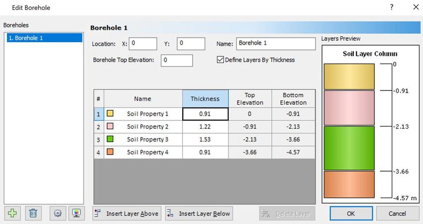
TABLE OF CONTENTS

ABSTRACT ................................................................................................................... ii

ACKNOWLEDGMENTS ............................................................................................ iii

LIST OF TABLES ........................................................................................................ vi

LIST OF FIGURES ..................................................................................................... vii

CHAPTER 1 – INTRODUCTION .................................................................................1

CHAPTER 2 – LITERATURE REVIEW ......................................................................3

 2.1 Loads and Damping in an OWT ...........................................................................3

 2.2 Hysteretic Damping in Soils .................................................................................6

 2.3 Hysteretic Damping in Axially Loaded Piles........................................................7

CHAPTER 3 – METHODOLOGY ..............................................................................12

 3.1 Test Sites .............................................................................................................12

 3.2 Analysis of Damping from Load Test Data ........................................................13

 3.2 Modeling Hysteretic Damping ............................................................................18

CHAPTER 4 – DISCUSSION AND RESULTS ..........................................................30

 4.1 Measured Results ................................................................................................30

 4.1.1 Dunkirk Pile ................................................................................................ 30

 4.1.2 URI Pile ....................................................................................................... 34

 4.2 Modeled Results ..................................................................................................37

 4.2.1 Dunkirk Pile ................................................................................................ 37

 iv

4.2.2 URI Pile ....................................................................................................... 40

CHAPTER 5 – SUMMARY AND CONCLUSION ....................................................44

APPENDICES ..............................................................................................................45

 APPENDIX A – MATLAB CODES ........................................................................45

 APPENDIX B – RS PILE INPUT DATA AND RESULTS ....................................50

BIBLIOGRAPHY .........................................................................................................54

 v

LIST OF TABLES

Table 1: Pile dimensions from the two test sites .......................................................... 13

Table 2: Soil Layers used for modeling at Dunkirk Site.............................................. 19

Table 3: Soil Layers used for modeling at URI Site .................................................... 19

Table 4: Relative density and soil friction angles used in the analysis at the Dunkirk Site

...................................................................................................................................... 21

Table 5: Parameters for API Model at Dunkirk Site .................................................... 22

Table 6: Relative density and interface friction angle used in the analysis at the URI Site

...................................................................................................................................... 23

Table 7: Parameters for API Model at URI Site .......................................................... 23

Table 8: Results of non-adjusted hysteresis loops at Dunkirk Site .............................. 31

Table 9: Results of adjusted hysteresis loops at Dunkirk Site ..................................... 32

Table 10: Results of non-adjusted hysteresis loops at URI Site .................................. 35

Table 11: Results of adjusted hysteresis loops at URI Site .......................................... 35

Table 12: Summary of modeling results at Dunkirk Site............................................. 42

Table 13: Summary of modeling results at URI Site ................................................... 43

 vi

LIST OF FIGURES

Figure 1: External loads acting on an offshore wind turbine (Nikitas, 2016) ................ 4

Figure 2: Illustration of an offshore wind Jacket structure showing (a) axial loading, and

(b) distributed spring model, and (c) lumped spring model (Bradshaw, 2022) ............. 5

Figure 3: Graphical illustration of shear modulus reduction and damping curves

(Bradshaw, 2022) ........................................................................................................... 6

Figure 4: Conceptual curves that are developed as part of the Analysis proposed by

Bradshaw (2022) ............................................................................................................ 8

Figure 5: CPT data from the Dunkirk Site (Bradshaw and Coulson, 2018) ................ 12

Figure 6: CPT data from the URI Site (Keefe et al. 2021) .......................................... 13

Figure 7: Typical load test data presented in Jardine and Standing (2000) ................. 14

Figure 8: Non-adjusted loops at Dunkirk ..................................................................... 15

Figure 9: Cycling loading loops at URI Site ................................................................ 16

Figure 10: Non-adjusted vs. adjusted loop for URI Site .............................................. 16

Figure 11:Non-adjusted vs. adjusted loop for Dunkirk Site ........................................ 17

Figure 12: Relative density of sand at Dunkirk Site (Jardine & Standing, 2000) ........ 21

Figure 13: Relative Density of sand at URI Site (Keefe, 2020)................................... 23

Figure 14: Estimation of the interface friction angle (Lehane et. al 2007) .................. 26

Figure 15: Grain size distribution curves at the URI Site (Keefe, 2020) ..................... 26

Figure 16: Typical output of the matlab program ........................................................ 28

Figure 17: Typical RS Pile results for the test pile at the URI Site ............................. 29

Figure 18: Plot of damping vs. cyclic load of field data at Dunkirk Site ..................... 33

 vii

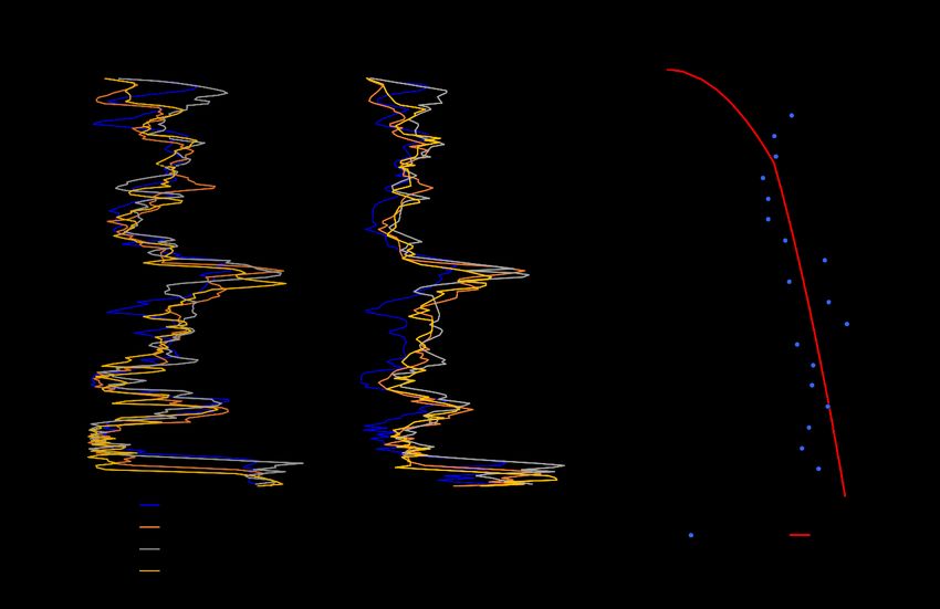
Figure 19: Plot of damping vs. cyclic displacement of field data at Dunkirk Site ...... 33

Figure 20: one way adjusted data vs. two way adjusted data for loops at Dunkirk Site

...................................................................................................................................... 34

Figure 21: Plot of damping vs. cyclic load of field data at URI Site ........................... 36

Figure 22: Plot of damping vs. cyclic displacement of field data at URI Site ............. 37

Figure 23: Load displacement curve for Dunkirk Site ................................................. 38

Figure 24: Plot of damping vs. cyclic load of modeled and measured data at Dunkirk

...................................................................................................................................... 39

Figure 25: Plot of damping vs. cyclic displacement (D-z curve) of modeled and

measured data at Dunkirk............................................................................................. 39

Figure 26: Load displacements curves for URI Site .................................................... 40

Figure 27: Plot of Damping vs. Cyclic Load of Modeled & Measured Data at URI Site

...................................................................................................................................... 41

Figure 28: Plot of damping vs. cyclic displacement (D-z curve) of modeled and

measured data at URI Site ............................................................................................ 41

Figure 29: Matlab Code of Measured Data for both Sites ........................................... 45

Figure 30: Soil properties API Method at URI Site ..................................................... 50

Figure 31: Soil properties UWA Method at URI Site .................................................. 50

Figure 32: Borehole at URI Site .................................................................................. 51

Figure 33: Pile properties for URI Site ........................................................................ 51

Figure 34: Soil properties API Method at Dunkirk Site (RS pile) ............................... 52

Figure 35: Soil properties UWA method at Dunkirk Site (RS pile) ............................ 52

Figure 36: Borehole Dunkirk Site (RS pile) ................................................................ 53

 viii

Figure 37: Pile properties at Dunkirk Site (RS pile) .................................................... 53

 ix

CHAPTER 1 – INTRODUCTION

As more and more offshore wind turbines (OWT) are being constructed in the United

States, is important to consider the environmental loads needed for design. These loads

are cyclic or dynamic in nature and can occur during normal operation as well as during

extreme events such as hurricanes. For a jacket structure, the loads from wind and waves

are mainly resisted by the axial capacity of the supporting piles.

Damping, which is the dissipation of energy stored in a dynamic system, has an

important role in the dynamic response of the structure. Typically, damping is ignored

in the design of piles for jacket structures but can possibly reduce the loads in the

structure, thereby extending the fatigue life. This thesis will focus on the hysteretic

damping, which is important at the typical vibration frequencies experienced by an

OWT.

A simple methodology was recently proposed by Bradshaw (2022) to estimate the

hysteretic damping of an axially loaded pile. The framework is based on a ‘t-z’ analysis,

which is commonly used to design piles for axial loading. In the approach the ‘t-z’

curves are developed from well-established empirical equations for modulus reduction

and damping ratio, which were developed from a database of dynamic element test

results. The damping ratio at the pile head is calculated through integration of the

dissipated energy and strain energy density within the deformed soil.

 1

The objective of this thesis was to test the validity of the proposed approach. This was

accomplished through analysis and modeling of existing cyclic pile load test data from

two test sites in the literature. The sites were located in Dunkirk, France and Davisville,

Rhode Island. The damping ratio of the test pile at the pile head was calculated for the

load tests by calculating the area within the hysteresis loops. The damping ratio was

also estimated for the test piles using the proposed modeling approach and the results

were compared.

Chapter 2 presents a brief literature review of the importance of static and dynamic

behavior of soil, dynamic loading, stiffness, and different methods that were used.

Chapter 3 is devoted to explaining the methodology to obtain the hysteretic damping

both for the analysis of the load test data as well as the numerical modeling. Chapter 4

presents and compares the measured and modeled hysteretic damping. Chapter 5

provides a summary and conclusions.

 2

CHAPTER 2 – LITERATURE REVIEW

This chapter presents a review of the literature that is relevant to this study.

2.1 Loads and Damping in an OWT

There exist four main sources of loads that act on an offshore wind turbine, which are

shown in Figure 1, and include the wind load, wave load, rotor load (1P) and blade

passing load (3P). They all have different characteristics in terms of amplitude and

frequency content. The wind and wave load can occur in different directions and at

different times. The rotor load is caused by mass and aerodynamic imbalances. The 3P

load is caused by the blades that are passing by the tower creating a wind shadowing

effect on the tower. These loads create cyclic vertical, horizontal, and moment reactions

on the supporting piles. The frequencies of the loads are on the order of 0.1 Hz for waves

loads to upwards of 0.3 to 0.6 Hz for the blade passing frequency (Bradshaw, 2022).

There are different damping mechanisms that occur within an Offshore Wind Turbine

(OWT) structure, including (Versteijlen, 2011):

- Aerodynamic Damping: caused by the turning rotor and due to movement of the tower

in the air

- Sloshing Damper: this is a system that uses a moving mass to dampen the vibrators

- Structural Damping: structural vibrations cause friction in the microcracks of the steel

leading to energy dissipation in the form of heat

- Soil Damping: material damping combined with geometric damping or radiation of

mechanical waves in the soil

 3

- Hydrodynamic Damping: viscous damping by the water around the OWT

Of the different mechanisms, the soil damping has some of the largest contributions but

perhaps is the most uncertain and difficult to predict. Hysteretic damping is frequency

independent and therefore, occurs at all frequency ranges. Geometric damping is

frequency dependent becoming more significant at frequencies above about 1 Hz

(Carswell et al. 2015). Since most OWT vibrations will be below 1 Hz many previous

studies have only focused on hysteretic damping.

 Figure 1: External loads acting on an offshore wind turbine (Nikitas, 2016)

As part of the design process, dynamic structural analyses are performed to approximate

the natural frequencies and evaluate the structural loads. In a jacket structure the lateral

loads acting on the structure are transferred into axial ‘push-pull’ loads on the piles. The

tensile loading on the pile is critical because the only resistance the pile has is through

skin friction (soil-pile shaft resistance) as seen in Figure 2a. If the load is in compression

then the structure also gets support through end-bearing resistance. As shown in Figure

 4

2, there are several ways how the stiffness (and damping) can be represented in a

dynamic model. However, it is common to conservatively neglect soil damping in

design. One way is shown in Figure 2b in which soil springs are assigned at different

points along the embedded length of the pile. This is commonly referred to as the

Winkler or ‘t-z’ approach and is commonly used in the analysis of OWT jacket

structures (Anoyatis et al. 2012, Michaelidis et. al. 1997). Although springs are shown

in the figure, soil damping could also be represented as dashpots or dampers also placed

at discrete points down the pile. A second way to represent the pile in a dynamic model

is shown in Figure 2c. Here the pile and soil are lumped together into an equivalent

spring (and dashpot) placed at the mudline level.

Figure 2: Illustration of an offshore wind Jacket structure showing (a) axial loading,
 and (b) distributed spring model, and (c) lumped spring model (Bradshaw, 2022)

 5

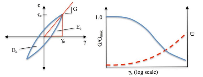
2.2 Hysteretic Damping in Soils

Hysteretic damping in soils refers to internal energy losses (i.e. dissipated energy)

within the soil mainly from inter-particle friction. Dynamic element tests, such as the

resonant column, can be used to measure hysteretic damping in soils. A typical cyclic

stress-strain curve of soil is shown in Figure 3. When the soil is exposed to symmetrical

cyclic loading, the stress-strain curve forms a loop for each cycle commonly referred to

as a ‘hysteresis loop’. The area within the hysteresis loop describes the energy dissipated

(Ee). It is common to describe these losses as a damping ratio defined by the following

equation:

 1 ℎ
 = (1)
 4 

Where Eh=dissipated energy per unit volume, and Ee= elastic strain energy per unit

volume. The secant shear modulus (G) can also be defined by taking the slope of the

stress strain loops at the points of load reversal. As shown on the right side of Figure 3,

the damping ratio and shear modulus are commonly presented as normalized modulus

and damping curves plotted against cyclic shear strain.

 Figure 3: Graphical illustration of shear modulus reduction and damping curves
 (Bradshaw, 2022)

 6

2.3 Hysteretic Damping in Axially Loaded Piles

The analytical response for a single pile subjected to dynamic vertical loads has been

shown in El Naggar and Novak (1994), Michaelides (1997) & Novak (1974) to name a

few. These approaches are largely theoretical and represent both geometric and/or

hysteretic damping in a variety of ways. Recently, Bradshaw (2022) proposed a simple

approach to estimate hysteretic damping in piles by integrating the dissipated and elastic

strain energy densities throughout the deformed soil mass. The advantages of the

method are that it (i) uses well-established modulus reduction and damping curves

developed for earthquake site response analyses, and (ii) the analysis is performed

within a ‘t-z’ framework, which is commonly used for pile design in engineering

practice. Since the method will be used later in the thesis, the details are presented below

using Figure 4 as an example.

 7

Figure 4: Conceptual curves that are developed as part of the Analysis proposed by
 Bradshaw (2022)

The first step is to construct the interface shear stress-axial displacement curve, also

called the ‘t-z’ curve shown in Figure 4a. The pile is assumed to be embedded in an

elastic soil and a vertical slice is considered forming an elastic whole-space with a hole

for the pile. The pile interface shear stress acts on the inside of the hole and the shear

stress at any point in the elastic material is calculated by the following:

 8

 0
 = 0 (2)
 
Where τ=shear stress at some radial distance r, 0 =interface shear stress, 0 =pile radius,

r=radial distance, F=function depending on loading frequency, radial distance, and soil

shear wave velocity. At the frequencies of interest for an OWT, F=1. Also, the elastic

space is broken up into concentric slices and the following equation is used to estimate

the shear stress at a given slice:
 0
 = 0 (3)
 
where =shear stress on a slice i, 0 =interface shear stress, 0 =pile radius, and =radial

distance to slice i. The secant shear modulus is estimated for each slice using the

following equation:

 = [ ] (4)
 
where =small strain shear modulus, [ ]=normalized modulus which depends
 
on the applied strain level. can be estimated using any number of modulus
 
reduction curves from the literature. The shear strain in each slice is therefore calculated

from the following basic definition:
 
 = (5)
 
The displacement of the pile is obtained through integration of the shear strains in the

radial direction:

 9

 

 = ∑ Δ (6)
 =1

where =pile interface displacement, =total number of slices, and Δ =radial width

of the slice. The ‘t-z’ curve is defined as 0 versus .

The next step is to construct the damping curve. For each level of applied interface shear

stress (and shear strain), the following equations are used to calculate the average elastic

strain energy density and dissipated energy density at a point representing the average

value within each radial slice:

 1
 = (7)
 2 

 ℎ = 4 (8)

where =elastic strain energy density in slice i, and ℎ =dissipated energy density in

slice i, and =damping ratio in slice i. The damping ratio can be estimated using any

number of damping curves available in the literature. Now integrating this across all

slices gives the following:
 
 ∗ = ∑ 2 Δ (9)
 =1

 ℎ∗ = ∑ 2 Δ ℎ (10)
 =1

 10

where ∗ =elastic energy per unit length of pile, ℎ∗ =dissipated energy per unit length of

pile, =radial distance to slice i. The ∗ and ℎ∗ varies with displacement as shown in

Figure 4b.

The damping ratio at the pile head is obtained by integrating the energy per unit length

with depth down the pile:

 1 ∑ ∗
 =1 ℎ ℎ 
 = (11)
 4 ∑ ∗
 =1 ℎ 

 ∗ ∗
where =number of soil layers, = average elastic energy in layer j, and ℎ =

average dissipated energy in layer j, ℎ =height of layer j.

 11

CHAPTER 3 – METHODOLOGY

The goal of this chapter is to provide a description of the pile load test sites, the analysis

of the pile load test data, and modeling of the test piles.

3.1 Test Sites

The test pile data that were used in this thesis were obtained from two previous field

studies that focused on the axial cyclic behavior of pipe piles in sands. The first study

site was located in Dunkirk, France as summarized in Jardine and Standing (2000). The

second site was located in Davisville, RI as summarized in Keefe (2020) and Keefe et

al. (2021). The Cone PenetrationTest (CPT) data from both sites are shown in Figures

5 and 6.

 Figure 5: CPT data from the Dunkirk Site (Bradshaw and Coulson, 2018)

 12

Figure 6: CPT data from the URI Site (Keefe et al. 2021)

The dimensions of the piles are summarized in Table 1. Note that the piles at Dunkirk

are much closer to full scale. All load tests were performed on open-ended pipe piles in

tension for both monotonic and one-way cyclic loading.

Table 1: Pile dimensions from the two test sites

 Dunkirk URI

 Length (m) 19.32 4.57

 Wall Thickness (mm) 13.5 6.35

 Radius (m) 0.2375 0.057

3.2 Analysis of Damping from Load Test Data

The data from Keefe (2021) were available electronically and thus could be imported

directly to Matlab for processing. The data from Jardine and Standing (2000) were not

available electronically so the data were digitized from the printed figures using the

 13

program Plot Digitizer that was available with a free license. An example of the data

showing the hysteresis loops is shown in Figure 7.

 Figure 7: Typical load test data presented in Jardine and Standing (2000)

As shown in Figure 7 not all the hysteresis loops could be digitized because of overlap.

Therefore, only the loops that were clearly identifiable were digitized resulting in up to

6 loops on each of 7 different test piles.

The values were taken evenly on each side of the loop. Afterwards the values were

modified in Excel. For plotting, the axes were flipped such that the X-Axis had

displacement [m or mm], and the Y-Axes had load [kN or kPa]. This can be seen in

Figure 8, where the loop in the middle was forcedly closed and therefore shifted to the

left side.

 14

Figure 8: Non-adjusted loops at Dunkirk

Due to the one way loading in tension, the loops contained some permanent

displacement. The permanent displacement was removed using the procedure proposed

by Lovholt (2019). This involved a linear incremental shifting of the displacements such

that the end point of the loop (point B on Figure 9) matched the starting point of the

loop (point A on the same figure). Therefore the distance marked “c” on the figure is

the permanent displacement.

 15

Figure 9: Cycling loading loops at URI Site

An example the adjusted loops are shown in Figures 10 (URI) and 11 (Dunkirk) for both

sites. If this correction was not done, the area, damping and secant stiffness would have

incorrect values for later comparisons.

 Figure 10: Non-adjusted vs. adjusted loop for URI Site

 16

Figure 11:Non-adjusted vs. adjusted loop for Dunkirk Site

A MATLAB code was developed (Appendix A) to calculate the area within a given

hysteresis loop and to calculate the secant stiffness. The program uses the trapezoidal

rule to numerically integrate the data. The following equations were used to calculate

the area within the loop:

 ( ) + ( + 1)
 ( ) = ( ) ( ( + 1) − ( )) (12)
 2

where = current step [-], = small area within two values, = force, load [kN], =

displacement [m]. The area within the loop was then calculated:

 = ∑ ( ) (13)

 17

where DW = sum of the small areas [kNm]. The elastic energy was calculated by the

following equation:

 1 ( ( ) − ( )) ( ( ) − ( ))
 = (14)
 2 2 2

with W = area under the shear modulus (G) [kNm]

The damping ratio D [%] was calculated from the following equation:

 1 
 = 100 [%] (15)
 4 

Finally, the stiffness k [kN/m] of the system was calculated by equation:

 max ( ) − min ( )
 = (16)
 max ( ) − min ( )

3.2 Modeling Hysteretic Damping

The goal of the modeling effort was to make a prediction of the hysteretic damping ratio

of the test piles and the pile head. The modeling process involved five steps including:

(1) developing a design soil profile, (2) estimating the unit shaft friction, (3) calculating

t-z and energy curves, (4) performing t-z analysis, and (5) calculating the damping ratio

at the pile head. The details of these steps are discussed in subsequent subsections.

Step 1. Develop Design Soil Profile

At each test site, CPT data were used to develop a design soil profile for the analysis

and summarized in Table 2 and 3. The soil at both test sites is sandy soil.

 18

Table 2: Soil Layers used for modeling at Dunkirk Site

 Depth of Layer Thickness Depth to midpoint average qc

 [m] [m] of layer z [m] [kPA]

 0-3 3 1.5 17122

 3-9 6 6 11677

 9-11 2 10 17480

 11-14 3 12.5 22090

 14-15.5 1.5 14.75 23848

 15.5-17 1.5 16.25 24048

 17-18.5 1.5 17.75 15195

 18.5-20 1.5 19.25 18623

Table 3: Soil Layers used for modeling at URI Site

 Depth of Layer Depth to midpoint average qc
 Thickness [m]
 [m] of layer z [m] [kPa]

 0 – 0.91 0.91 0.455 3043

 0.91 – 2.13 1.22 1.52 5358

 2.13 – 3.66 1.53 2.895 9096

 3.66 – 4.57 0.91 4.115 20374

 19

Step 2. Estimate Unit Shaft Friction

Two methods were used in this thesis to calculate the unit shaft friction including the

API ‘Main Text’ method and the UWA-05 method. These methods and input parameters

are described below.

API Method

The unit shaft resistance determines the maximum interface shear stress in the t-z curve.

The API (2007) ‘Main Text’ method was used to estimate the unit shaft resistance as

follows:

 = ′ = ′ tan( ′ ) (17)

Where = shaft friction factor chosen of Table 6.4.3-1 from API (2007) by the density

of each soil layer, ′ = vertical effective stress at the layer midpoint of each layer, =

lateral earth pressure coefficient, ′ = peak soil-pile interface friction angle, assuming

the pile is drained during loading. For steel interfaces, the interface friction angle is

typically taken as 2/3 of the peak friction angle of the soil. CPT correlations were used

to estimate the effective friction angle in each layer using Kulhawy and Mayne (1990):

 ( ⁄ )
 ′ = 17.6 + 11 log (18)
 ′
 (√ ⁄ )
 [ ]

With = toe resistance, ′ = effective stress and = atmospheric pressure (=100

kPa). The results are shown in Table 4.

 20

Figure 12: Relative density of sand at Dunkirk Site (Jardine & Standing, 2000)

Table 4: Relative density and soil friction angles used in the analysis at the Dunkirk Site

 Depth of Layer Soil Friction
 Dr [%] Density
 [m] Angle φ’[°]

 0-3 103 Very dense 45

 3-9 60 Medium dense 41

 9-11 76 Dense 42

 11-14 71 Dense 42

 14-15.5 77 Dense 42

 15.5-17 70 Dense 42

 17-18.5 59 Medium dense 40

 18.5-20 53 Medium dense 41

 21

The static pullout pile capacity ( ) was calculated from the following equation:

 = ∑ (19)

Therefore, for the Dunkirk Site a summary of the most important parameters are shown

in Table 5. The ultimate pullout capacity is the sum of the shaft resistance with is here

for the modelled pile 1528 kN.

Table 5: Parameters for API Model at Dunkirk Site

 Vertical
 Pile Shaft
 Effective fmax Gmax
 z [m] Beta [-] Surface Resistance
 Stress σ’v [kPa] [kPa]
 Area [m2] [kN]
 [kPa]

 1.5 26 0.56 14 4.31 62 41355

 6 89 0.37 33 8.61 282 88301

 10 129 0.46 59 2.87 170 105944

 12.5 154 0.46 71 4.31 305 115652

 14.75 177 0.46 81 2.15 175 122290

 16.25 192 0.46 88 2.15 190 127013

 17.75 207 0.37 77 2.15 165 132306

 19.25 222 0.37 82 2.15 177 136683

The process was repeated for the URI site. The results are summarized in Tables 6 and

7. The pullout capacity of the pile was estimated to be about 17 kN.

 22

Figure 13: Relative density of sand at URI Site (Keefe, 2020)

Table 6: Relative density and interface friction angle used in the analysis at the URI
Site

 Depth of Layer Soil Friction
 Dr [%] Density
 [m] Angle φ’[°]

 0-0.91 48 Medium Dense 40

 67 70 Dense 41

 2.13 – 3.66 83 Dense 42

 3.66 – 4.57 82 Dense 45

Table 7: Parameters for API Model at URI Site

 Vertical
 Pile Shaft
 Effective fmax Gmax
 z [m] Beta [-] Surface Resistance
 stress σ’v [kPa] [kPa]
 2
 Area [m ] [kN]
 [kPa]

 23

0.455 8.95 0.37 3.31 0.326 1.08 9191

 1.522 14.85 0.46 6.83 0.437 2.98 24619

 2.895 28.14 0.46 12.95 0.548 7.09 88847

 4.115 39.94 0.46 18.37 0.326 5.99 104694

UWA-05

The UWA-05 method uses CPT data directly to estimate static pile capacity. The

method is summarized in Lehane et al. (2007) and Randolph and Gouvernec (2011) and

the equations are summarized below.

 0.2
 = min [1, ( ) ] (20)
 1.5

Where IFR = the incremental filling ratio and = the inner pile diameter,

 2
 = 1 − ( ) (21)
 0

 = effective area ratio , 0 = outer pile diameter. The radial effective stress after pile

installation is found by following equation:

 −0.5
 2 ℎ
 ′ = max ( , 2) (22)
 0

 24

Where = the CPT uncorrected cone tip resistance, = the stress drops from qc around

the pile tip (Randolph and Gourvenec, 2011), = the effective area ratio described

 ℎ
below, and is a relation of the pile’s slenderness ratio, otherwise defined as a ratio of
 0

height above the pile tip to outside pile diameter. The value, a, is taken as 0.03 for open

ended piles in tension.
 
 ( ⁄ )
 1 = 0.5 (23)
 ′
 ( ⁄ )

 = [185( 1 )−0.75 ] (24)

Where G = soil shear modulus, = uncorrected cone tip resistance and 1 = cone tip

resistance normalized by effective overburden stress. Normal stress changes due to

shear band dilation were estimated using the following:

 4 
 ( 0.02)
 0 (25)
 Δ ′ =
 1000

Where ∆ ′ = the change in radial effective stress due to shear band expansion.

 = 0.75( ′ + Δσ′ )tan ( ′ ) (26)

Where ′ = the constant volume friction angle of the soil. The capacity was determined

the same way as the API method.

 25

The constant volume interface angle for the Dunkirk site was taken as 27° throughout

all layers as measured in interface shear tests. For the URI site, the constant volume

interface angle was estimated from Figure 14. The D50 was selected for each layer based

on the grain size curves shown in Figure 15.

 Figure 14: Estimation of the interface friction angle (Lehane et. al 2007)

 Figure 15: Grain size distribution curves at the URI Site (Keefe, 2020)

 26

Step 3: Generate t-z and Energy curves

Dr. Bradshaw developed a Matlab program to make the calculations and the code is

presented in the Appendix. It is based on Equations 2 through 11. The damping ratio

per unit volume was calculated using the modulus reduction and damping curves

developed by Ishibashi and Zhang (1993). For a given pile, the calculations were

performed for each of the layers in the soil profile. The key input parameters include

the unit shaft friction, soil friction angle, small strain shear modulus, and heterogeneity

coefficient. The heterogeneity coefficient is defined by the following (Randolph and

Wroth 1978):

 /2
 ρ= (27)
 
Where GL/2= shear modulus halfway down the pile, and GL= shear modulus at the pile

toe. Based on the Gmax profiles a value of 0.7 was used for URI and 0.77 for Dunkirk.

The output is the t-z curve, dissipated and elastic strain energy per unit length of pile,

and the damping ratio for the layer. A typical result from one of the soil layers for the

URI pile is shown in Figure 15.

 27

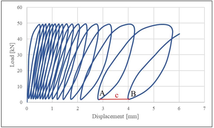
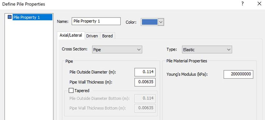
Figure 16: Typical output of the matlab program

Step 4: Perform T-Z Analysis

RS Pile software was used to perform the t-z analysis. The input parameters are the pile

dimensions soil properties and the t-z curves for each layer. An axial tensile load was

applied in increments to the pile head and the resulting pile displacements were

calculated at the pile head and at the midpoint of each layer. An example of the RS Pile

displacement output is shown in Figure 17 for the URI site. All RS-Pile files and data

are also presented in the Appendix. Whereas the soil layers were defined in Table 6 ,

the ground water table is at 0.91 m and the different colours next to the pile show axal

displacement.

 28

Figure 17: Typical RS Pile results for the test pile at the URI Site

Step 5: Calculate the Damping Ratio at Pile Head

The pile displacements calculated at the midpoint of each layer were used to select the

dissipated energy and elastic energy for each layer using the curves generated in Step 3

(Figure 16b). The damping ratio at the pile head was calculated from Equation 11.

 29

CHAPTER 4 – DISCUSSION AND RESULTS

4.1 Measured Results

4.1.1 Dunkirk Pile

The results interpreted from the load test data are summarized in Tables 8 and 9 and

plotted in Figures 18 and 19. The adjusted loops have a lower damping ratio than the

raw loops whereas the stiffness is higher in the adjusted loops. The damping ratio of the

adjusted loops ranged from 4% to 46%. Generally, the damping ratio does not appear to

correlate with the applied load level but increases with an increase in cyclic

displacement. This is consistent with typical soil behavior that shows that damping ratio

increases with increasing cyclic strain.

 30

Table 8: Results of non-adjusted hysteresis loops at Dunkirk Site

 Cyclic Cyclic
 Average
Pile Test Code Loop Load Displacement DW [Nm] W [Nm] D [%] k [kN/m]
 Load [kN]
 [kN] [mm]
 1 897.7 448.9 4.5 4.4 2.1 16.6 205.9
 R3 CY3 2 950.6 475.3 5.6 8.1 2.6 24.4 166.0
 3 1120.4 560.2 9.2 21.2 4.3 38.9 101.6
 R4 CY3 1 1210.1 605.1 4.1 4.1 1.6 20.5 185.1
 1 1195.7 597.9 3.3 2.3 1.2 15.0 228.6
 R5 CY2
 2 1217.3 608.7 3.7 3.8 1.4 22.1 203.6
 1 654.6 327.3 3.3 1.8 1.1 13.0 209.6
 2 639.2 319.6 3.4 2.3 1.2 15.5 206.3
 3 753.2 376.6 4.6 5.7 1.6 28.7 149.7
 R5 CY 3
 4 756.9 378.5 4.9 6.7 1.7 31.8 140.7
 5 844.1 422.0 5.6 8.6 1.9 35.7 122.6
 6 745.3 372.6 6.4 10.3 2.2 37.0 109.1
 1 742.7 371.3 4.6 8.6 1.6 43.0 150.3
 2 734.8 367.4 4.7 8.9 1.6 43.7 144.8
 R6 CY 4 3 690.1 345.1 4.7 8.8 1.6 43.5 148.2
 4 725.6 362.8 6.5 13.4 2.3 47.4 105.3
 5 711.7 355.8 4.7 9.0 1.6 44.2 145.2
 1 -10.3 -5.1 9.1 -14.0 2.7 41.2 65.8
 C1 CY 1 2 -38.7 -19.3 9.7 -15.1 2.9 41.6 61.8
 3 47.1 23.5 9.9 -14.7 3.0 39.8 60.6
 1 -83.5 -41.7 2.5 -1.8 0.5 26.7 167.9
 2 -66.2 -33.1 2.8 -2.8 0.5 40.8 136.1
 3 -90.7 -45.4 3.6 -3.8 0.7 43.6 106.8
 4 -30.5 -15.2 4.8 -5.5 0.9 47.7 78.4
 5 -17.6 -8.8 9.4 -11.7 2.0 47.2 44.1
 C1 CY 3
 6 -11.8 -5.9 11.0 -12.3 2.3 42.7 37.7
 7 -20.1 -10.1 11.6 -12.6 2.4 41.5 36.3
 8 -18.7 -9.3 12.2 -13.0 2.6 40.6 34.3
 9 -15.6 -7.8 11.5 -12.2 2.4 40.2 36.6
 10 -9.2 -4.6 9.5 -9.5 2.0 38.3 44.0

 31

Table 9: Results of adjusted hysteresis loops at Dunkirk Site

 Cyclic
 Average Cyclic
Pile Test Code Loop Displacement DW [Nm] W [Nm] D [%] k [kN/m]
 Load [kN] Load [kN]
 [mm]
 1 898.8 449.4 4.2 3.2 2.0 12.8 221.3
 R3 CY3 2 951.1 475.5 4.6 4.6 2.2 17.0 202.5
 3 1122.8 561.4 6.2 8.3 2.9 22.6 151.2
 R4 CY3 1 1195.9 598.0 3.7 1.9 1.4 10.7 206.4
 1 1198.9 599.4 3.0 1.4 1.1 9.4 245.7
 R5 CY2
 2 1219.3 609.6 3.2 1.8 1.2 11.7 233.6
 1 654.4 327.2 3.0 1.2 1.0 9.6 231.5
 2 638.2 319.1 3.0 1.4 1.0 11.1 230.5
 3 754.1 377.1 3.4 2.6 1.2 17.9 204.8
 R5 CY 3
 4 756.9 378.5 3.4 3.2 1.2 21.4 200.7
 5 844.1 422.0 3.7 3.3 1.3 20.6 186.6
 6 751.0 375.5 4.1 4.7 1.4 26.3 170.4
 1 744.1 372.1 3.5 5.6 1.2 37.4 199.1
 2 734.3 367.2 3.7 6.1 1.3 38.4 187.4
 R6 CY 4 3 690.5 345.3 3.5 5.8 1.2 38.4 197.1
 4 726.5 363.3 4.3 7.4 1.5 39.7 160.2
 5 712.1 356.0 3.6 6.0 1.2 38.8 191.5
 1 -12.3 -6.2 8.6 -13.9 2.6 43.2 69.0
 C1 CY 1 2 -38.7 -19.3 8.7 -14.9 2.6 45.5 68.5
 3 42.3 21.2 8.7 -15.0 2.6 46.4 68.8
 1 -84.7 -42.4 2.6 -1.8 0.5 26.2 165.8
 2 -66.2 -33.1 2.8 -2.8 0.5 40.7 135.9
 3 -90.7 -45.4 3.6 -43.7 0.7 43.7 107.3
 4 -30.5 -15.2 4.8 -5.5 0.9 47.7 78.5
 5 -20.8 -10.4 9.4 -11.6 2.0 47.3 44.1
 C1 CY 3
 6 -18.2 -9.1 10.1 -12.2 2.1 46.3 40.9
 7 -22.7 -11.4 10.4 -12.5 2.2 45.8 40.3
 8 -23.2 -11.6 10.9 -12.8 2.3 44.9 38.2
 9 -20.8 -10.4 10.1 -12.0 2.1 45.2 41.4
 10 -18.4 -9.2 8.1 -9.3 1.7 44.3 50.9

 32

50
 45 non-adjusted loops
 40 adjusted loops
 35

 Damping [%]
 30
 25
 20
 15
 10
 5
 0
 0 100 200 300 400 500 600 700
 Cyclic Load [kN]

 Figure 18: Plot of damping vs. cyclic load of field data at Dunkirk Site

As shown in Figure 18 the adjusted loops have a lower damping then the non- adjusted

loops. The adjusted loops have a smaller area when closed and therefore is the damping

also smaller because it is the area in between the hysteresis loop. Following this the

stiffness is decreasing. The ranges of the cyclic loading are between 300 and 600 kN .

 Figure 19: Plot of damping vs. cyclic displacement of field data at Dunkirk Site

 33

When looking at Figure 19 the displacement of the adjusted loops have almost a linear

relationship between damping ratio and displacement.

Figure 20: one way adjusted data vs. two way adjusted data for loops at Dunkirk Site

In Figure 20 are the adjusted loops (adjusted) compared for both the one way and two

way loading tests. It shows that the cyclic displacement is higher during the two way

loading tests then the one way loading tests.

4.1.2 URI Pile

The results interpreted from the URI load test data are summarized in Tables 10 and 11

and plotted in Figures 21 and 22. The damping ratio of the adjusted loops ranged from

12% to 40%. Similar trends are observed with cyclic load and displacement as Dunkirk.

 34

Table 10: Results of non-adjusted hysteresis loops at URI Site
 Average Cyclic Cyclic
Pile Test Cyclic Loading Stage Loop Load Load Displacement DW [Nm] W [Nm] D [%] k [kN/m]
 [kN] [kN] [mm]
 1 1.9 0.9 3.2E-02 4.2E-05 2.6E-05 13.0 50.4
 Stage 1 2 2.0 1.0 2.7E-02 5.2E-05 2.0E-05 20.8 54.8
 3 2.0 1.0 2.8E-02 5.7E-05 2.0E-05 22.1 52.9
 4 2.3 1.1 4.1E-02 6.6E-05 3.9E-05 13.5 46.4
 Stage 2 5 2.3 1.2 4.2E-02 7.9E-05 4.2E-05 15.1 46.9
 6 2.2 1.1 4.1E-02 1.0E-04 4.0E-05 20.0 47.9
 7 2.8 1.4 5.4E-02 1.1E-04 6.2E-05 14.0 43.0
 Pile 2 Stage 3 8 2.7 1.4 5.1E-02 1.6E-04 5.9E-05 21.0 45.5
 9 2.6 1.3 4.7E-02 1.4E-04 5.6E-05 20.1 49.4
 10 2.9 1.5 7.2E-02 2.9E-04 1.1E-04 21.5 41.5
 Stage 4 11 3.0 1.5 6.3E-02 1.7E-04 8.3E-05 16.6 42.1
 12 3.0 1.5 6.1E-02 2.3E-04 8.2E-05 22.0 43.4
 13 3.5 1.8 1.2E-01 8.1E-04 1.8E-04 35.3 24.4
 Stage 5 14 3.4 1.7 2.1E-01 2.0E-03 3.1E-04 51.5 13.8
 15 3.3 1.7 2.4E-01 2.4E-03 3.5E-04 54.8 11.9

Table 11: Results of adjusted hysteresis loops at URI Site
 Average Cyclic Cyclic
Pile Test Cycling loading Stage Loop Load Load Displacement DW [Nm] W [Nm] D [%] k [kN/m]
 [kN] [kN] [mm]
 1 1.9 0.9 3.2E-02 4.4E-05 2.6E-05 13.3 50.2
 Stage 1 2 1.9 1.0 2.6E-02 4.9E-05 2.0E-05 19.8 56.5
 3 1.9 1.0 2.7E-02 5.5E-05 2.0E-05 21.9 53.2
 4 2.2 1.1 4.2E-02 8.0E-05 3.9E-05 16.1 45.3
 Stage 2 5 2.4 1.2 4.2E-02 7.3E-05 4.1E-05 14.2 46.7
 6 2.2 1.1 4.1E-02 1.0E-04 3.9E-05 20.5 47.7
 7 2.9 1.5 5.3E-02 9.2E-05 6.0E-05 12.2 43.1
 Pile 2 Stage 3 8 2.8 1.4 4.9E-02 1.3E-04 5.7E-05 18.6 46.1
 9 2.6 1.3 4.9E-02 1.6E-04 5.7E-05 22.5 48.0
 10 2.9 1.5 7.4E-02 3.1E-04 1.1E-04 22.6 40.4
 Stage 4 11 3.0 1.5 6.2E-02 1.7E-04 8.2E-05 16.5 42.3
 12 3.0 1.5 6.1E-02 2.2E-04 8.1E-05 22.1 43.6
 13 3.5 1.8 9.6E-02 4.4E-04 1.4E-04 24.6 31.3
 Stage 5 14 3.4 1.7 1.4E-01 2.1E-04 1.0E-03 38.7 20.8
 15 3.4 1.7 1.6E-01 1.1E-03 2.2E-04 40.5 18.2

 35

Figure 21: Plot of damping vs. cyclic load of field data at URI Site

The damping is increasing with the cyclic load. Also is shown when more cyclic load is

happening the Damping has a bigger discrepancy of the non-adjusted loops towards the

adjusted loops. Most of the tests war taken between a load of 1-1.5 kN. Therefore, most

of the damping is happening between 10 and 25%.

 36

Figure 22: Plot of damping vs. cyclic displacement of field data at URI Site

In Figure 22 the cyclic behavior of the displacement is linear, and the Damping ratio is

increasing linearly with the cyclic displacement. Most of the tests had a Damping ratio

of 10-25%.

4.2 Modeled Results

In the following sections, the modeled data are compared to the field data.

4.2.1 Dunkirk Pile

Figure 23 compares the modeled and measured monotonic load-displacement behavior.

The modeled and measured ultimate capacities were consistent. The API model had a

higher estimated capacity then the UWA model. The good agreement gives additional

confidence in the t-z model.

 37

Figure 23: Load displacement curve for Dunkirk Site

The developed results for cyclic loads of the Dunkirk pile are summarized in Table 12.

The modeled results are compared with the measured damping in Figures 24 and 25 for

the Dunkirk site. The modeled damping ratio generally fell on the lower end of the

measured results.

 38

Figure 24: Plot of damping vs. cyclic load of modeled and measured data at Dunkirk

 Figure 25: Plot of damping vs. cyclic displacement (D-z curve) of modeled and
 measured data at Dunkirk

 39

4.2.2 URI Pile

The monotonic load displacement curves for the URI pile are shown in Figure 26. As

shown in the figure, the modeled capacities are significantly higher than the measured

capacities. As described in Keefe et al. (2021) the lower than expected capacity was

likely due to friction fatigue during pile driving which was magnified by the small pile

diameter.

 Figure 26: Load displacements curves for URI Site

A summery of the cyclic modeling results is presented in Table 13. The modeled results

are compared with the measured damping in Figures 27 and 28 for the URI site. The

modeled damping ratio generally fell on the lower range of measured results.

 40

Figure 27: Plot of Damping vs. Cyclic Load of Modeled & Measured Data at URI Site

 Figure 28: Plot of damping vs. cyclic displacement (D-z curve) of modeled and
 measured data at URI Site

 41

Table 12: Summary of modeling results at Dunkirk Site

 API Model UWA Model

 Cyclic Cyclic
 Cyclic Damping Cyclic Damping
 Displacement Displacement
 Load [kN] RAtio[%] Load [kN] Ratio [%]
 [mm] [mm]

 0 0 0 0 0 0

 100 5.56 0.44 100 5.70 0.4467

 200 8.65 0.95 200 9.00 1.0217

 300 10.98 1.55 300 11.06 1.8168

 400 10.05 2.36 400 12.15 2.7585

 500 9.82 3.26 500 12.89 3.889

 600 10.03 4.26 600 14.53 5.902

 700 10.49 5.49 612.5 22.60 18.18

 725 10.77 11.39

 42

Table 13: Summary of modeling results at URI Site

 API model UWA model

 Cyclic Cyclic
 Cyclic Damping Cyclic Damping
 Displacement Displacement
 Load [kN] Ratio [%] Load [kN] Ratio [%]
 [mm] [mm]

 2.50 3.63 0.04 2.5 12.13 0.22

 5 6.46 0.10 5 18.40 0.50

 7.50 7.58 0.16 7.5 20.98 0.85

 8.50 19.71 0.95 10 23.28 1.30

 8.75 25.73 8.33 11 23.65 1.49

 9 25.73 20.19 12 28.42 6.49

 43

CHAPTER 5 – SUMMARY AND CONCLUSION

The objective of this thesis was to test the validity of a newly proposed approach to

estimate the damping ratio of an axially loaded pile. This was accomplished through

modeling and analysis of existing cyclic pile load test data from two test sites in the

literature. The sites were located in Dunkirk, France and Davisville, Rhode Island. The

damping ratio of the test pile at the pile head was calculated for the load tests by

calculating the area within the load-displacement hysteresis loops. The damping ratio

was also estimated for the test piles using the proposed modelling approach and the

results were compared. Both the measured and modeled results show that damping

increases with cyclic displacement. The model underpredicts the measured damping at

all cyclic displacement and cyclic load levels. The results are promising in that the

proposed model might be useful for providing a lower bound and thus conservative

estimate of damping as the model ignores interface slippage up to the point where the

maximum shaft resistance is reached., which would increase the damping.

 44

APPENDICES

 APPENDIX A – MATLAB CODES

Matlab code used to calculate damping ratio and stiffness from the measured pile load

test data

 Figure 29: Matlab Code of Measured Data for both Sites

 45

Matlab code used to model the t-z and energy curves.

 46

47

48

49

APPENDIX B – RS PILE INPUT DATA AND RESULTS

 Figure 30: Soil properties API Method at URI Site

 Figure 31: Soil properties UWA Method at URI Site

 50

Figure 32: Borehole at URI Site

Figure 33: Pile properties for URI Site

 51

Figure 34: Soil properties API Method at Dunkirk Site (RS pile)

Figure 35: Soil properties UWA method at Dunkirk Site (RS pile)

 52

Figure 36: Borehole Dunkirk Site (RS pile)

Figure 37: Pile properties at Dunkirk Site (RS pile)

 53

BIBLIOGRAPHY

Anoyatis, G., & Mylonakis, G. (2012). Dynamic Winkler modulus for axially loaded
piles. Geotechnique, 62(6), 521-536.

Bradhsaw, A.; Coulson, R. (2018). Axial cyclic degradation of marine piles: a strain-
based fatigue limit

Bradshaw, A. (2022) “Approach to Estimate Hysteretic Soil Damping in Piled Jacket
Structures.” Proceedings of the ASCE 2022 ASCE Geo-Congress. (in press).

Bryden, C., Arjomandi, K., & Valsangkar, A. (2018). Effect of material damping on the
dynamic axial response of pile foundations. In Proc., 6th Int. Structural Specialty Conf.
Fredericton, NB, Canada: Canadian Society for Civil Engineers.

Bryden, C., Arjomandi, K., & Valsangkar, A. (2020). Dynamic axial response of tapered
piles including material damping. Practice Periodical on Structural Design and
Construction, 25(2), 04020001.

Carswell, W., Johansson, J., Løvholt, F., Arwade, S. R., Madshus, C., DeGroot, D. J.,
& Myers, A. T. (2015). Foundation damping and the dynamics of offshore wind turbine
monopiles. Renewable energy, 80, 724-736.

White, D. J., Clukey, E. C., Randolph, M. F., Boylan, N. P., Bransby, M. F., Zakeri, A.,
& Jaeck, C. (2017, May). The state of knowledge of pipe-soil interaction for on-bottom
pipeline design. In Offshore Technology Conference. OnePetro.

Damgaard, M., Ibsen, L. B., Andersen, L. V., & Andersen, J. K. (2013). Cross-wind
modal properties of offshore wind turbines identified by full scale testing. Journal of
Wind Engineering and Industrial Aerodynamics, 116, 94-108.

El Naggar, M. H., & Novak, M. (1994). Non-linear model for dynamic axial pile
response. Journal of geotechnical engineering, 120(2), 308-329.

Gazetas, G., & Makris, N. (1991). Dynamic pile‐soil‐pile interaction. Part I: analysis of
axial vibration. Earthquake Engineering & Structural Dynamics, 20(2), 115-132.

Gupta, B. K., & Basu, D. (2018). Dynamic analysis of axially loaded end-bearing pile
in a homogeneous viscoelastic soil. Soil Dynamics and Earthquake Engineering, 111,
31-40.

Ishibashi, I., & Zhang, X. (1993). Unified dynamic shear moduli and damping ratios of
sand and clay. Soils and foundations, 33(1), 182-191.

 54

Jardine, R. J., & Standing, J. R. (2000). Pile load testing performed for HSE cyclic
loading study at Dunkirk, France. V. 1.

Jardine, R. J., & Standing, J. R. (2012). Field axial cyclic loading experiments on piles
driven in sand. Soils and foundations, 52(4), 723-736.

Kramer, S. L. (1996). Geotechnical earthquake engineering. Pearson Education India.

Lehane, B. M., Schneider, J. A., & Xu, X. (2005). The UWA-05 method for prediction
of axial capacity of driven piles in sand. Frontiers in offshore geotechnics: ISFOG, 683-
689.

Loukidis, D., Salgado, R., & Abou-Jaoude, G. (2008). Assessment of axially-loaded
pile dynamic design methods and review of INDOT axially-loaded pile design
procedure.

Løvholt, F., Madshus, C., & Andersen, K. H. (2019). Intrinsic Soil Damping from
Cyclic Laboratory Tests with Average Strain Development. Geotechnical Testing
Journal, 43(1), 194-210.

Menq, F. Y. (2003). Dynamic properties of sandy and gravelly soils. The University of
Texas at Austin.

Michaelides, O., Gazetas, G., Bouckovalas, G., & Chrysikou, E. (1998). Approximate
non-linear dynamic axial response of piles. Geotechnique, 48(1), 33-53.

Novak, M. (1974). Dynamic stiffness and damping of piles. Canadian Geotechnical
Journal, 11(4), 574-598.

Poulos, H. G. (1988). Cyclic stability diagram for axially loaded piles. Journal of
geotechnical engineering, 114(8), 877-895.

Randolph, M. F., Jeer, H. A., Khorshid, M. S., & Hyden, A. M. (1996, May). Field and
laboratory data from pile load tests in calcareous soil. In Offshore Technology
Conference. OnePetro.

Randolph, M. F., & Wroth, C. P. (1978). Analysis of deformation of vertically loaded
piles. Journal of the geotechnical engineering division, 104(12), 1465-1488.

Randolph, M., & Gourvenec, S. (2011). Offshore Geotechnical Engineering. CRC
press.

Trochartis, A. M., Bielak, J., & Christiano, P. P. (1987). Hysteretic dissipation of piles
under cyclic axial load. Journal of geotechnical engineering, 113(4), 335-350.

 55

Versteijlen, W. G., Metrikine, A., Hoving, J. S., Smidt, E. H., & De Vries, W. E. (2011).
Estimation of the vibration decrement of an offshore wind turbine support structure
caused by its interaction with soil. In Proceedings of the EWEA Offshore 2011
Conference, Amsterdam, The Netherlands, 29 November-1 December 2011. European
Wind Energy Association.

 56