Computer vision enables short- and long-term analysis of Lophelia pertusa polyp behaviour and colour from an underwater observatory - Uni Bielefeld
←
→
Page content transcription
If your browser does not render page correctly, please read the page content below
www.nature.com/scientificreports

                         OPEN      Computer vision enables short-
                                   and long-term analysis of Lophelia
                                   pertusa polyp behaviour and colour
Received: 8 August 2018
Accepted: 4 March 2019             from an underwater observatory
Published: xx xx xxxx
                                   Jonas Osterloff 1, Ingunn Nilssen2, Johanna Järnegren3, Tom Van Engeland                        4,6
                                                                                                                                         ,
                                   Pål Buhl-Mortensen5 & Tim W. Nattkemper 1
                                   An array of sensors, including an HD camera mounted on a Fixed Underwater Observatory (FUO) were
                                   used to monitor a cold-water coral (Lophelia pertusa) reef in the Lofoten-Vesterålen area from April
                                   to November 2015. Image processing and deep learning enabled extraction of time series describing
                                   changes in coral colour and polyp activity (feeding). The image data was analysed together with data
                                   from the other sensors from the same period, to provide new insights into the short- and long-term
                                   dynamics in polyp features. The results indicate that diurnal variations and tidal current influenced
                                   polyp activity, by controlling the food supply. On a longer time-scale, the coral’s tissue colour changed
                                   from white in the spring to slightly red during the summer months, which can be explained by a
                                   seasonal change in food supply. Our work shows, that using an effective integrative computational
                                   approach, the image time series is a new and rich source of information to understand and monitor the
                                   dynamics in underwater environments due to the high temporal resolution and coverage enabled with
                                   FUOs.

                                   Because of their high biodiversity and importance as habitat for fish, the cold-water coral (CWC) reefs receive
                                   much attention from academia and authorities as well as NGO’s and the general public1,2. CWC habitats are
                                   commonly found in deep waters, often far from shore, and accessing these systems is challenging. Despite
                                   the challenges, CWC in the North East Atlantic and US-waters are reasonably well studied, on shorter time
                                   scales. In the NE Atlantic, the stony coral Lophelia pertusa is the dominant CWC reef builder3,4, forming large
                                   three-dimensional structures that provides habitat for many other species. In addition to its function as biological
                                   hotspot, CWC reefs also play an important part in biogeochemical cycles and processing of organic matter in the
                                   deep-sea5–7.
                                       Forty years ago, knowledge on geographical distribution of CWC reefs was only based on reported by-catch
                                   from fishermen, in addition to a limited number of surveys3. Active knowledge gathering provided by academia
                                   and industry has traditionally been based on physical sampling by dredging and/or grabbing8–10. Such sampling
                                   methods are destructive for the sampled organisms and the habitat. Furthermore they do not collect all groups of
                                   reefs associated species in a representative way11.
                                       With increased use of remotely operated vehicles (ROV) in the 1980s, it became possible to study the seafloor
                                   and its habitats and organisms directly. Several CWC reefs were discovered during seafloor mapping and pipe-
                                   line surveys for the Norwegian offshore oil and gas industry12. The Sula reef, the Morvin field and the Breisund
                                   area are examples of the latter3 (and the MAREANO on-line map service: www.mareano.no). However, despite
                                   extensive mapping and visual surveys in some geographical areas, knowledge about the distribution of these
                                   ecosystems worldwide is still limited.

                                   1
                                     Biodata Mining Group, Faculty of Technology, Bielefeld University, PO Box 33501, Bielefeld, Germany. 2Equinor,
                                   Research and Technology, 7005, Trondheim, Norway. 3Norwegian Institute for Nature Research, P.O. Box 5685
                                   Torgarden, 7485, Trondheim, Norway. 4NIOZ Royal Netherlands Institute for Sea Research, Department of Estuarine
                                   and Delta Systems, Utrecht University, Korringaweg 7, 4401NT Yerseke, the Netherlands. 5Research Group Benthic
                                   Habitat, Institute of Marine Research, 5817, Bergen, Norway. 6Department of Biology, Ecosystem Management
                                   Group, University of Antwerp, Universiteitsplein 1, 2610, Wilrijk, Belgium. Correspondence and requests for
                                   materials should be addressed to T.W.N. (email: tim.nattkemper@uni-bielefeld.de)

        Scientific Reports |   (2019) 9:6578 | https://doi.org/10.1038/s41598-019-41275-1                                                            1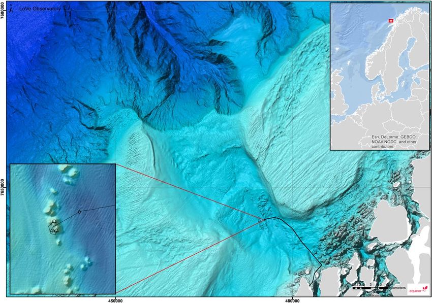
www.nature.com/scientificreports/                                                              www.nature.com/scientificreports

                           Figure 1. The location of the LoVe observatory. Map generated using Esri ArcGIS 10.2.2 for Desktop.
                           Bathymetry data downloaded from Mareano (http://www.mareano.no/kart/mareano.html#maps/3192) and
                           publicly available. Display of infrastructure data granted by Equinor.

                                From present knowledge it seems that geographic location and local conditions, such as prey availability and
                           depth, influence the diet13. In some locations CWC appear to mainly be feeding on zooplankton13–15. In coastal
                           and oceanic waters in northern Norway copepods are by far the most dominant group within the mesozooplank-
                           ton, and the most important herbivorous planktotrophic species is the copepod Calanus finmarchicus16. Wax ester
                           serve as the storage lipid in C. finmarchicus and can comprise up to 50% of this copepod’s dry weight17. Calanus
                           finmarchicus also contains the carotenoid astaxanthin18, which is a red pigment often used as a food dye to attain
                           coloration in cultivated salmonids and crustaceans19.
                                In addition to the visual documentation with mobile sensor platforms, an increasing number of fixed under-
                           water observatories (FUO) are equipped with digital cameras. This way visual information with high temporal
                           resolation can be collected over a large time period in order to monitor small areas in CWC ecosystems. The
                           in-situ image collections have the potential to provide new insights in ecosystem processes and natural environ-
                           mental variations on both short (hours and days) and long term (seasons and years). The polyp behaviour of L.
                           pertusa has previously been studied to further understand the biology of the coral and to investigate the possi-
                           bility of using the polyps as an indicator of stress20–23. In general, the polyp behaviour reflects feeding patterns,
                           and probably other physiological processes3,24. During a petroleum drilling campaign in the Norwegian sea in
                           2009–2010, the first attempt to measure polyp activity of CWC from a fixed platform in situ was made23.
                                Computational support is necessary to efficiently process and interpret the huge amounts of image data gath-
                           ered both from mobile platforms and fixed ocean observatories. This computational support ranges from data
                           management and development of databases to complex analyses such as image enhancement, segmentation
                           and classification. An additional advantage of computerized image analyses is their objectivity and repeatabil-
                           ity. Analyses conducted by humans frequently have low intra-/inter- observer agreement25. This problem may
                           be caused by human selective vision and limitation in dividing attention to a variety of simultaneous informa-
                           tion26,27, such as detecting different organisms and/or their movements over time. Furthermore, detecting small
                           scale changes in object features, such as colour change, is hard for the human brain without a proper scale or
                           colour reference. Several studies have documented that observers have considerable difficulties in recognizing
                           changes in colour or orientation, in particular, when distracting patterns can influence the subjects’ visual atten-
                           tion (see for instance28,29).
                                At present, only a limited number of approaches for computational marine image analysis has been presented.
                           Previous studies have solved different image analysis tasks, such as CWC segmentation in ROV images30,31
                           coral classification32, marine resource assessment33,34 or megafauna classification35–37. Computational meth-
                           ods for image data from stationary observatories have been developed to solve tasks such as object detection/
                           screening38,39, monitoring of shrimp distribution in and underneath a L. pertusa reef40, quantification of colour
                           change in L. pertusa over time41 and detection and classification of polyp activity in selected parts of a L. pertusa
                           reef42. Recently, also a short time series study has been published on the gorgonian coral Paragorgia arborea,
                           including manual assessment of visual features of the corals43. A comprehensive overview for underwater image
                           pre-processing can be found in44.
                                This study represents the next step, where images computationally extracted from a stationary observatory are
                           combined with other sensor data. Image time series and sensor data are obtained from the Lofoten-Vesterålen
                           (LoVe) ocean observatory (love.equinor.com). The aim of the data analyses is to identify and describe, if any,
                           short and long-term dynamics in the behaviour and visual features of L. pertusa. The main factors that might
                           influence the behavioural changes are discussed. Short-term dynamics refer here to short periods of hours to days
                           and long-term dynamics are defined as period of months or the total time period analysed, about seven months.

Scientific Reports |   (2019) 9:6578 | https://doi.org/10.1038/s41598-019-41275-1                                                             2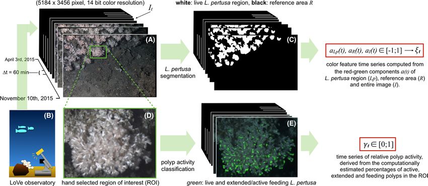
www.nature.com/scientificreports/ www.nature.com/scientificreports
Original temporal
Feature resolution Sensor name Supplier
Temperature f t(T) [° Celsius] 60 min AADI 4319A/ADII 4117D Aanderaa
Depth f t(D) [m] 60 min AADI 4319A/ADII 4117D Aanderaa
Conductivity f t(C) [mS/cm] 60 min AADI 4319A Aanderaa
Salinity f t(S) [PSU] 60 min AADI 4319A Aanderaa
Chlorophyll 60 min Seapoint Chlorophyll Fluorometer Seapoint sensors inc.
Current velocity north f t(Vn1) [m/s] 10 min Nortek AS
ADCP Aquadopp and ADCP Continental
Current velocity east f t(Ve1)[m/s] 10 min (only the second was used in the final Nortek AS
Current velocity vertical f t(Vu1) [m/s] 10 min analysis due to the higher time coverage Nortek AS
with the analyzed time-period)
Current velocity horizontal f t(Vh1) [m/s] 10 min Nortek AS
Coral color ξt 60 min Image based Nortek AS
Polyp activity γt 60 min Image based Nortek AS
Table 1. The temporal resolution of the different sensors ft used in the multivariate data analysis. Further
details can also be found in the online documentation (https://love.statoil.com/Resources/LoVe%20Ocean%20
Observatory%20Sensor%20System.pdf).
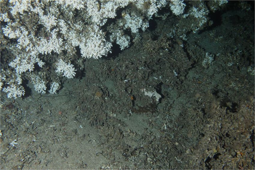
Figure 2. An image recorded at the LoVe observatory the 4th of April 2015 05:59. In the upper left part of the
image mostly live CWC can be found, in contrast to the lower right parts where mostly dead coral fragments
appear. In between the live coral reef and the coral sand, a coral rubble area were small coral fragments are
mixed with sand can be seen.
Material and Field Applications
The study area. The Lofoten-Vesterålen (LoVe) ocean observatory is located at approximately 250 m depth
about 12 km (i.e. ∼20 nautical miles) off the coast of Northern Norway (N 68°54.474′, E 15°23.145′, see Fig. 1).
The location is a biological hot spot area in the Norwegian sea, hosting the main spawning area for the North
Atlantic cod and has more than 300 L. pertusa reefs45.
Equipment and sensors. The ocean observatory was deployed in October 2013. In addition to a waterproof
housing (METAS DSF5210) for a digital camera (Canon EOS 550D) and a flash (METAS DSF 4365), the obser-
vatory is equipped with a range of sensors (see Table 1 for an overview). In our study, environmental data such
as salinity, conductivity, temperature, depth, current speed and direction, and chlorophyll, were correlated with
polyp activity. The camera was oriented at an angle of 45° towards a L. pertusa reef. The camera covered a visual
field of approximately 10 m2, including both live parts of the reef and coral rubble as shown in Fig. 2. One image
with a resolution of 5184 × 3456 pixels was recorded per hour.
Current velocity data were checked for consistency of measurement between the two available ADCPs (Nortek
Aquadopp and Nortek Continental) in the overlapping part of their range. ADCP alignment was compared
with readings from an independent compass (OASITILT sensor cf. online documentation on the data portal).
Environmental sensor data (temperature, salinity/conductivity) were checked for quality using internal consist-
ency checks of the equipment (e.g. comparison of temperature series from the AADI device with that accessory
sensors from the ADCPs). Data recorded at the LoVe FUO is publicly available and can be downloaded from
http://love.equinor.com.
Scientific Reports | (2019) 9:6578 | https://doi.org/10.1038/s41598-019-41275-1 3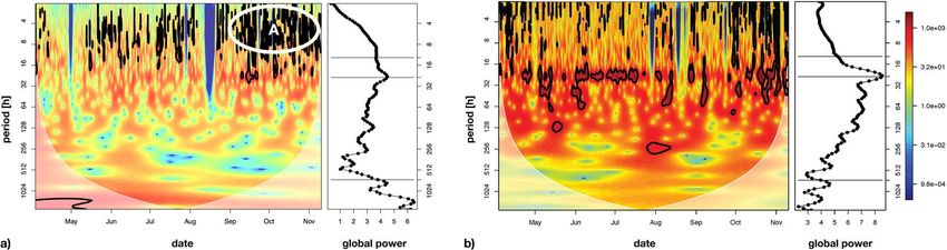
www.nature.com/scientificreports/                                                                     www.nature.com/scientificreports

                           Figure 3. One image (see (A)) per hour is uploaded from the LoVe observatory (see schematic graph (B),
                           image drawn by author TWN) to the web portal. To compute a time series of colour values (see upper row),
                           the image region of live L. pertusa is determined in every single image using a segmentation algorithm (see
                           (C) and text for details). Inside the region covered with L. pertusa, as well as for the entire image It, the average
                           colours are computed in the CIELab colour space, with the three coordinates L (=luminance), a (=red-green
                           component) and b (=yellow-blue component). The a-coordinates of the L. pertusa region for all time points
                           were used as time series ξt to describe the red-green component of the considered L. pertusa area (see white
                           mask in (C)) throughout the observation period. To represent the percentage of active polyps at one time point
                           γt (see lower row) the polyp activity classification algorithm (see the text for details) was applied to each hand
                           selected observation field of view (D) to estimate the amount of extended and feeding polyps (green area in (E)).

                           Methods
                           The image sequence from the LoVe observatory which is considered in this study consists of 4862 images {I1, …,
                           IN} recorded in the time from April 3rd to November 10th, 2015. In order to extract coral features time series of
                           interest, we used two machine learning based algorithmic approaches that were applied to each image It. The first
                           approach was used to compute a coral colour feature ξt for each image and time point that describes the colour of
                           the coral. The second approach was used to describe the relative polyp activity γt for each image. The approaches
                           are described briefly in the following. A detailed description of all processing steps is also given for both meth-
                           ods in the Supplementary Materials S1 and S2. Additional information can be found in41,42. An overview for the
                           computational extraction of both the image-derived time series is shown in Fig. 3. The image analyses have been
                           implemented using the software packages OpenCV (http://openCV.org), NVIDIA DIGITS (http://developer.
                           nvidia.com/digits) and the CAFFE framework (http://caffe.berkeleyvision.org) as well as C++ code developed
                           by the Biodata Mining Group, Bielefeld University. Afterwards we describe the application of linear regression
                           and wavelet coherence analysis that was used to investigate linear relationships between the different time series
                           and their periodicities.

                           Coral colour time series computation. Monitoring the corals’ colour change requires automated extrac-
                           tion of colour features from the digital photos that represent the CWC colour at time point t (a more detailed
                           description for this method is given in the Supplementary Method S1). First, all images are spatially aligned46 and
                           colour transformed (i.e. It → I ′t ) with a fixed white balancing. After this pre-processing step, pixel-labelling
                           based segmentation is applied in order to compute a binary mask image M   ˆ coral for the live corals (see Fig. 3 upper
                           middle). The pixel labelling function is constructed using a hierarchical hyperbolic self-organizing map30,47,
                           which is trained with Gabor features from a small subset of the images. Then, we computed for each image I ′t the
                           average CieLab colour values48 for the full image (i.e. all pixels)
                                                                                          w       h
                                                                                 1
                                                                    ctfull =        ⋅    ∑ ∑ I ′t ,(x ,y )
                                                                                w⋅h      x =1 y =1                                              (1)
                           and for the live coral colour
                                                                                           w      h
                                                                                 1
                                                                    ct full =       ⋅     ∑ ∑ I ′t ,(x ,y )
                                                                                w⋅h       x =1 y =1                                             (2)
                           (i.e. only for the pixels inside the mask, see Fig. 3, top right). As the L- and the b-values did not show any variation
                           of interest we chose the coral colour time series to be the a-channel of the live coral colour ct coral as it encodes the
                           complementary red-green component:

                                                                                 ξt = ct ,coral
                                                                                          a .                                                   (3)

Scientific Reports |   (2019) 9:6578 | https://doi.org/10.1038/s41598-019-41275-1                                                                 4
www.nature.com/scientificreports/ www.nature.com/scientificreports
Polyp activity time series computation. A time series γt describing the relative polyp activity (feeding
vs. non-feeding) was computed (and a more detailed description can be found in the Supplementary Method S2).
To this end, a region of interest (ROI) was chosen that showed CWC with sufficient contrast and in focus (see
green frame and lower row in Fig. 3). After pre-processing the images, 13 image ROIs were displayed to human
experts (i.e. the authors JJ, IN, PB) to mark positions of active polyps and inactive ones using the annotation soft-
∼
ware BIIGLE 2.049,50. Based on the three users’ point annotations, a binary mask M inside the ROI was deter-
∼
mined that describes the locations of all polyps (i.e. M = 1, for all polyp pixels and = 0, otherwise). In order to
train, validate and test a deep neural network, image patches of equal size (46 × 46) were extracted at the positions
marked by the human experts, that summed up to 2410 image patches showing polyps. A background class was
∼
generated by extracting 100 image patches at random locations in the same ROI but outside the mask M . The
number of training sample patches was further increased by flipping (augmentation factor: 2x) and rotating (aug-
mentation factor: 12x) the patches and by adding Gaussian noise to them to avoid overfitting (augmentation
factor: 2x). Employing these boosting procedures, we achieved a data augmentation by the factor of 48, i.e. an
increase of the training data volume by 48-times. Image patches for all categories (active/inactive polyp) are
divided into training (70%), validation (20%) and test (10%) patches. Training and validation set were used for
training and parameter optimization. The test was left out in in this step so it could be used for a final assessment
of the network’s performance for new and “unseen” data. A deep convolutional neural network with a LeNet-5
layout51 was trained for classifying image patches to feature an active polyp or an inactive one using the NVIDIA
∼
DIGITS software. To finally compute the polyp activity γt for one time point, all pixels (x, y) inside the mask M
are classified by the network to show an element of an active polyp or an inactive one. The network output C(p(x,y))
represents the likelihood of the image patch p(x,y) centered at pixel (x, y) showing an active polyp, i.e. C(p(x,y)) = 1)
or not (i.e. C(p(x,y)) = 0) for retracted polyps or other structures. The aggregated number of pixels classified to be
∼
“active” in relation to the size of the positive area in M gives the estimated percentage of active polyps for each
ROI It , referred to as polyp activity γt in the rest of this manuscript:
~
| {p(x , y ) ∈ It|C(p(x , y ) ) = 1}|
γt = ~ .
| M = 1| (4)
Multivariate data analysis. In order to investigate functional relations between the introduced
image-derived coral colour ξt (see eq. 3) and polyp activity γt (see eq. 4), and the other physical conditions meas-
ured by the other sensors ft (like temperature f t(T) or salinity f t(S)), several analyses were conducted. The different
sensors of the LoVe observatory have different sampling rates and show varying short episodes of sensor dysfunc-
tions, the latter additionally causing different kinds of temporal delays between measurements of different sen-
sors. Depending on the type of analysis, a mapping and/or interpolation for the different time series was required.
In the following we briefly describe the different methods of statistical data analysis we have applied.
To test linear correlations between the image derived time series (γt and ξt) and sensor time series we com-
puted a time series xt for each sensor ft that had the same temporal resolution as the image time series. Given an
original sensor time series ft and the original time points {t|ft ≠ ∅} of its measurements, we computed the new
sensor time series xt by interpolation
ft ≥ − ft ≤
xt = ⋅ (t − t ≤) + ft ≤ ,
t≥ − t≤ (5)
with
t ≤ = max{t ⁎|t ⁎ ≤ t ∧ t ⁎ ∈ {t|ft ≠ ∅}} (6)
and
t ≥ = min{t ⁎|t ⁎ ≥ t ∧ t ⁎ ∈ {t|ft ≠ ∅}} . (7)
Pairs of time-series were plotted in scatterplots to identify potential relationships between data sets. Linear
correlation was tested between polyp activity, γt and time series xt. Daily averages (γt , x t ) of γt and xt were com-
puted and tested for pair-wise correlation. For the latter, no linear interpolation was applied, ignoring days where
no data was recorded either for γt and/or xt.
Wavelet-based analysis methods were performed 1) to identify dominant frequencies/scales that contribute to
the overall variance in individual time series, and 2) to assess covariation between the image-derived time series
and the environmental variables measured by the other sensors. In contrast to a Fourier transformation-based
analysis, which discards the time dimension when data are transformed to frequency space, the wavelet trans-
formation retains time and frequency/scale information, thus facilitating identification of patterns in data that
have limited temporal extent52. Dominant frequencies/scales in individual time series were identified in the
bias-corrected wavelet power spectrum53,54. The default Chi2-test from the R function was used to test for sig-
nificance of variance contributions at the 95% significance level. Scale- and time dependent covariation between
two time series was investigated with a wavelet coherence analysis55. Wavelet coherence is the wavelet transfor-
mation analogue of a cross-correlation analysis or a Fourier coherence analysis. It is calculated from the wavelet
cross-spectrum of two series by dividing it by the power spectra of the individual time series56. It is reported as
a squared value between 0 and 1, similar in interpretation to a squared correlation. Significance of the wavelet
variance and coherence was tested by Monte Carlo randomization tests54.
Scientific Reports | (2019) 9:6578 | https://doi.org/10.1038/s41598-019-41275-1 5www.nature.com/scientificreports/ www.nature.com/scientificreports
Figure 4. Measurements of selected sensors are plotted together with estimated polyp activity γt and coral
colour ξt (a-coordinate of the coral colour ct coral). Plot (a) shows the development of the colour value ξt that
describes the redness of the color structures. An increase of ξt reflects a change of the colour into a more reddish
hue. In mid of May the colour starts to change into red. Plot (b) shows the corresponding relative polyp activity
at each time point γt. Gaps in the series originate in camera malfunctions. Plot (c) shows the temperature and
(d) the measured concentration of chlorophyll with a high peak at the end of April. In (e–h) the four plots of the
current velocity measurements are shown (with e) Ve1, (f) Vh1, (g) Vn1, (h) Vu1). Plot (i) shows the distance
from the bottom to the sea surface.
Since the methodology behind the biwavelet package assumes equidistant time points for the analysis of a time
series (and identical temporal resolution for a pairwise analysis) the time series must be transformed accordingly.
Estimated polyp activity γt, coral color ξt with the original time points of imaging {t|γt ≠ ∅} were therefore con-
verted to have equidistant time points (t = 1 hour) by linear interpolation:
γ t≥ − γ t≤
γ ′t = ⋅ (t − t ≤) + γ t ≤
t≥ − t≤ (8)
with
t ≤ = max{t ⁎|t ⁎ ≤ t ∧ t ⁎ ∈ {t|γt ≠ ∅}} (9)
and
t ≥ = min{t ⁎|t ⁎ ≥ t ∧ t ⁎ ∈ {t|γt ≠ ∅}} . (10)
To allow a pairwise analysis of image-derived time series with other sensor data ft was mapped ( ft → x ′t ) to
interpolate measurements for those time points of the set {t|γ ′t ≠ ∅}. The wavelet transformation was applied to
each individual time series with a Morlet mother wavelet function, followed by pairwise coherence wavelet anal-
ysis between γt and all xt. The analyses were conducted in the R Statistical software (R Core Team, 2016) using the
addon package “biwavelet”57.
Results
To assess the accuracy in polyp activity, several processing approaches were evaluated and compared. A com-
parison of the human expert annotations showed an inter-observer agreement of 0.86 and an intra-observer
agreement of 0.89. The classification accuracy of the trained network was 0.98 for the training data and 0.96 for
the validation and test data. The accuracy of the relative polyp activity γt was assessed for the 13 images, that were
annotated by the human experts (more details are given in the Supplementary S2). From the manual annotations,
another value for relative polyp activity was computed and compared to γt. A spearman’s rank correlation of the
two measurements was calculated to be 0.98.
An overview of all data attributes and temporal resolutions is given in Table 1. Raw data are displayed in
Fig. 4a–i. As can be seen in the plots, the time series show some gaps due to sensor problems and/or break downs
of the communication with the ocean observatory.
Nevertheless, the time series of polyp activity, coral colour as well as temperature and conductivity (data not
shown) show long-term trends and patterns with marked changes starting in May.
Scientific Reports | (2019) 9:6578 | https://doi.org/10.1038/s41598-019-41275-1 6www.nature.com/scientificreports/ www.nature.com/scientificreports
Figure 5. The daily averages for temperature ( x t(T)) are plotted against daily averages for the polyp activity (γt ).
The estimated pearson correlation coefficient between both is 0.54.
Figure 6. The wavelet power spectrum (see left panels in the subplots) of the polyp activity (γ′t ) (see a))
northward bottom current velocity (x t(Vn1)) (see b)) and the corresponding scale-averaged global power spectra
(right panels in the subplots). Significant contributions to the time series’ variance (Chi2-test, 95% significance
level) are indicated by the black contours. The horizontal lines in the global wavelet spectra mark the tidal scale
(12.4 h, daily (24 h) and lunar (~707 h) scales.
The colour value (ξt), describing the redness of the polyp tissue, changes gradually towards more reddish hue
from mid of May to August (Fig. 4a). The onset of this change seems to follow a marked peak in the chlorophyll
concentration at the end of April (Fig. 4d). The current velocity did not display any clear seasonality patterns
(Fig. 4e–h). The variation in depth reflects the tidal variation (Fig. 4i).
Polyp activity γt increased rapidly between a bottom water temperature 7.4 and 7.5 °C and reached a maxi-
mum between 7.5 and 8.0 °C (Fig. 5). At higher bottom water temperatures polyp activity decreased slightly to
remain more or less constant beyond temperatures of 8.3 °C (Fig. 5). Pearson correlation coefficients
(Supplementary Table S3) for pairwise correlation of γt and x t(C ), x t(T ), x t(S) were not high. The estimated coeffi-
cients for the daily average were higher but still below 0.8. Looking at the correlation between polyp activity and
current, r(γt , x t(Vu1)) and r( γ t I , x t(Vu1)), the values indicated no linear dependency.
The periodicity of the different time series was analysed using wavelet transformations. Linear interpolation
was used to compute time series with equidistant time points from γt and ft (see equation (8)). First, single time
series were analysed with respect to periodic patterns, starting with the polyp activity γt. The result of this analysis
is visualized in Fig. 6a.
The wavelet spectrum of the polyp activity γt exhibited only statistically significant variance contributions at
scales below 16 hours (black contours in Fig. 6a (left panel), plots without the black contours are shown in the
Supplementary S4). These statistically significant regions occurred throughout summer, but particularly from
September to November (region indicated with “A” in Fig. 6a), left panel). Although no significant variance con-
tribution in poly activity γt was detected at the 24-hour scale band in the wavelet variance plot (Fig. 6a, left
panel), the corresponding global wavelet variance spectrum (right panel in Fig. 6a), averaged by scale, exhibited
a distinct peak at the 24-hour scale, indicating that polyps showed some increased variation in feeding activity
with a 24-hour scale. Additional variance peaks were also found at longer scales, including that of the lunar cycle
(approx. 700 h = ~29 days).
The wavelet spectral plot (Fig. 6b (left panel), a plot without black contours is shown in the Supplementary S4)
and global averaged wavelet spectrum (Fig. 6b, right panel) of the northward component of the bottom current
velocity (Vn1) showed a significant and dominant contribution of the 24-hour scale to the overall variance, indic-
ative of a tidal dominance in the current velocity. A bit surprisingly, no spectral peaks were found at the 12.5 h
scale, which may be due to interactions of the tidal wave with the basin morphology. Some significant contribu-
tions of smaller time scales were found as well but were mainly restricted to the beginning and end of the time
series.
Similar analyses of the wavelet variance demonstrated a strong contribution of the lunar phase to the overall
variance in the eastward current velocity component and a dominant tidal (12.5 h) contribution to the water
depth (data not shown).
Scientific Reports | (2019) 9:6578 | https://doi.org/10.1038/s41598-019-41275-1 7www.nature.com/scientificreports/ www.nature.com/scientificreports
Figure 7. Left panel: Squared wavelet coherence (colour) and phase (arrows) between polyp activity (γ ′ t ) and
′
the northward component of the bottom current velocity (x (Vn1) ). A value of 1 would indicate a perfect
t
coherence, while a value of 0 would indicate no coherence. Significant coherence is indicated by the black
contour lines (Monte Carlo test, 95% significance level). Right panel: The corresponding scale-averaged
coherence over the entire measurement period.
Significant coherence (covariation) between the polyp activity and the northward current velocity was found
at various scales up to 256 hours (~10 days), throughout the entire measurement period (Fig. 7 (left panel) and
Supplementary Fig. S5). At the 24-hour scale the two signals tended to be in phase (arrows predominantly point-
ing to the right in Fig. 7 left panel), whereas they tended to be in counter-phase at larger scales (arrows predom-
inantly pointing to the left).
In the Supplementary Fig. S6 we show a plot of polyp activity and current velocity Vn1 for a selected interval
of 4 weeks to illustrate coherences (see Supplementary Fig. S3).
Discussion
Our results show that the polyp behavior of the monitored L. pertusa display different, alternating temporal pat-
terns, or periodicities. The analyses indicate that the main factors influencing the polyp behavior and color varies
both with respect to the internal relationship between the various factors measured and with time. Behavioral
periodicity has been observed in many warm water corals (see references in58) but such patterns have not been
previously documented in CWC in situ.
Long term dynamics. In general, the long-term (7 months) trend of polyp activity and coral color
(Fig. 4a,b) follow a similar pattern with a low level from April to May, followed by a gradual increase from May
to July. The onset of the increase follows an early sharp peak in chlorophyll content (Fig. 4d). This peak marks the
spring bloom of phytoplankton, which is the basis for the growth of the zooplankton communities, dominated
by calanoid copepods. The long-term change in the colour in the L. pertusa reef (Fig. 4a) was first published in
201638,41 and is further supported by our study. We suggest that the colour changes documented in L. pertusa
between April and November, is a result of increased feeding on calanoid copepods containing the red pigment
astaxanthin. According to13 and15, copepods and other planktonic animals within reach of the reefs during sum-
mer constitute the main food sources for L. pertusa together with phytodetritus59,60. The increased polyp activity
is likely to be related to feeding activity, and as a high food uptake continues throughout the summer and early
fall, the pigments from the food probably accumulate in the coral tissue. Changes in polyp activity related to
feeding activity has previously been documented in laboratory experiments61,62. The calanoids show both sea-
sonal and diurnal vertical migration patterns. During winter, the populations enters diapause in deep and cold
water. Patches of high abundance of overwintering C. finmarchicus in the Lofoten Basin, just west of our study
site, has been documented at 550–800 meters63. In mid-late winter, the population ascends to surface waters
where it matures and spawns (see for example64). During its life cycle C. finmarcicus goes through six Nauplius
and five Copepodite stages (CI-CV). The maximum abundance of the first generation CI often occur during or
right after the peak of the phytoplankton bloom (reviewed in65). In June and July, the first generation of CIV and
CV starts to migrate into the deep for diapause and a second generation starts their migration in August and
September16,63,66,67.
In addition to the seasonal migration, the calanoid perform diurnal vertical migration (DVM). This is a strat-
egy to avoid visual predators (e.g. fish)68–70. Copepods reside deeper in the water column during the day than at
evening and night time, when they migrate towards the sea surface to graze on phytoplankton (e.g.66).
With the maturation of the calanoids, the depth of the migration increases towards the end of the sum-
mer16,66,69 before it is followed by the migration to diapause. The CWC habitats in Norway are relatively shallow71
and it is therefore likely that the seasonal migration, in combination with the DVM, accommodate the CWC with
high quality food during summer and autumn.
Scientific Reports | (2019) 9:6578 | https://doi.org/10.1038/s41598-019-41275-1 8www.nature.com/scientificreports/ www.nature.com/scientificreports
Our suggestion that copepods are causing the colour change in L. pertusa is further supported by16, showing
that the storage lipid signature of L. pertusa contained a higher level of calanoid copepod lipid biomarkers at
the shallow Mingulay reef (130 m) than the deeper reefs at Rockall (900 m) and New England (1200–1300 m).
Additionally, the Mingulay corals contained the highest number of wax esters of the sites, which is the storage
lipid of the copepod C. finmarchicus17.
Temperature (Fig. 4c) also shows long-term seasonal changes, with a steady increase from April/May until end
of the measuring period in mid-November. Between May and September, there is a positive correlation (r2 = 0.54)
between polyp activity and temperature. Such a correlation has also been observed in laboratory experiment72.
However, from September until mid-November, the temperature continues to increase while the polyp activity
decreases. L. pertusa occur within a rather wide temperature range worldwide, from 4 to 14 °C, and has a high
tolerance to an unpredictable temperature regime73. This may suggest that food availability influence polyp activ-
ity to a higher degree than temperature. But given duration of the measurements and the lack of verification of
food available in the data, there are currently not enough data available to conclude on how the temperature or a
combination of temperature and food influences the polyp activity of L. pertusa. Analyses on longer time series
in the future will determine whether the correlation with temperature and other drivers at the seasonal scale
is of ecological significance or just an artefact of the cyclicity in two auto-correlating time series with a limited
temporal extent.
Short term patterns. The short term (hours and days) dynamics (i.e. short periodicities) of the different
sensors seem to be more complex than the long-term (months) changes controlled by factors varying both diur-
nally (Figs 6 and 7) and with the lunar phase (tidally).
The wavelet coherent study for current speed and polyp activity showed a match for 24 hours and an approx-
imate match for 33 days. The results from the coherence analysis suggest opposite responses of polyp feeding
activity to tidal currents relative to residual currents (larger than 24-hour). However, the coherence at the 24-hour
scale does not necessarily have to originate from tidal variability. Daily vertical migration of prey species could
also induce variability of polyp feeding activity at a 24-hour scale. From August onwards significant coherence
was also detected at the lunar scale. Signals were roughly in counter-phase at this scale.
Even though no long-term pattern was documented for current speed and direction in the present study, it is
documented that food transport to corals is directly linked to current speed and direction74. Laboratory studies
have shown that slow current speeds, with velocities less than 7 cm/sec, are optimal for feeding in CWC61,62. At
higher flow velocity fewer polyps are active, likely due to greater drag on the tentacles and lower probability of
food capture61,62. The authors of62 also describe the variety of food capture efficiency with food source in addition
to water flow. Furthermore, also a field study13 has indicated changes in the proportion of polyps in different
expansion states caused by natural stress from water motion around the polyps and/or by different water quality
or food content related to changes in current speed and direction.
The tidal wavelength of 12.25 hours is directly linked to variation in current speed and direction. Because of
a tidal periodicity of 12.25 hour, high and low tide does not occur at the same time every day. This implies that
there are days within this cycle when the currents are disadvantageous while the zooplankton is present around
the corals, and vice versa. During a tidal cycle, highest current velocities occur twice (6.12 hours apart). A combi-
nation of wave patterns can feature interferences and this may explain why the corals’ polyp behaviour seems to
swap between different periodicities (Fig. 6a).
Our findings demonstrate the importance of using a sampling frequency relevant for capturing dynamic pat-
terns at the scale they occur. Which time scale is relevant for sampling of biological and environmental data
depends on the aim of the study.
Conclusions and future perspectives. The high temporal resolution and coverage of the data measured at
the LoVe ocean observatory opens up for a new insight, and jet unknown opportunities for understanding natural
variations and the dynamic in CWC reefs. These first results reveal that various parameters influence L. pertusa at
different time scales, and that the various periodicities also influence each other.
Understanding the natural variations and dynamics influencing key species or ecosystems is essential to inter-
pret environmental monitoring data.
To gain more insight and knowledge about these interactions there is first and foremost a need to gather more
experience and better statistics for both long- and short-term changes. Furthermore, to generalize the present findings,
the methodology must be further developed for applications in broader areas. The results also show that to reduce the
uncertainty in our analysis there is a need of technology development of sensors that can measure and specify food
availability with high temporal frequency and coverage. The documentation of L. pertusa changing color through the
year is one example of new knowledge that is a result of interdisciplinary collaboration on the LoVe data.
In a broader perspective, the anticipation of L. pertusa feeding on C. finmarcicus causing this color change
indicates a strong predator-prey interaction between the two species. We can therefore expect that fluctuations
in zooplankton also could influence L. pertusa’s general health and reproductive cycles. With more than 10.000
L. pertusa reefs documented in Norwegian waters this new knowledge should also be considered included in
CWC ecosystem modelling. As indicated in this study L. pertusa might be an important predator that at present
is missing in the modelling. Ultimately, this new insight could also have implications for understanding details in
food web dynamics involving commercial important fish stocks grazing on copepods, such as herring.
Data Availability
All Images and sensor data used in this work were made available via the Lofoten-Vesterålen Ocean Observatory
web portal (love.statoil.com). The single time series are also provided with this submission (data_matrix.zip).
Scientific Reports | (2019) 9:6578 | https://doi.org/10.1038/s41598-019-41275-1 9www.nature.com/scientificreports/ www.nature.com/scientificreports
References
1. Buhl-Mortensen, P. Coral Reefs in the Southern Barents Sea: Habitat Description and the Effects of Bottom Fishing. Marine Biology
Research 13(10), 1027–40 (2017).
2. Costello, M. J. et al. Role of cold-water Lophelia pertusa coral reefs as fish habitat in the NE Atlantic. Cold-Water Corals and
Ecosystems. Springer Berlin Heidelberg, 771–805 (2005).
3. Mortensen, P., Hovland, T., Fosså, J. H. & Furevik, D. M. Distribution, abundance and size of Lophelia pertusa coral reefs in mid-
Norway in relation to seabed characteristics. Journal of the Marine Biological Association of the UK 81(4), 581–97 (2001).
4. Wheeler, A. J. et al. Morphology and environment of cold-water coral carbonate mounds on the NW european margin. International
Journal of Earth Sciences 96(1), 37–56 (2007).
5. Van Oevelen, D. et al. The cold-water coral community as a hot spot for carbon cycling on continentalmargins: A food-web analysis
from Rockall Bank (northeast Atlantic). Limnology and Oceanography 54, 1829–44 (2009).
6. Wagner, H., Purser, A., Thomsen, L., Jesus, C. C. & Lundälv, T. Particulate organic matter fluxes and hydrodynamics at the Tisler
cold-water coral reef. Journal of Marine Systems 85, 19–29 (2011).
7. White, M. et al. Cold-water coral ecosystem (Tisler Reef, Norwegian Shelf) may be a hotspot for carbon cycling. Mar. Ecol. Progr.
Ser. 465, 11–23, https://doi.org/10.3354/meps09888 (2012).
8. Dons, C. Norges Korallrev. Det Kongelige Norske Videnskabers Selskabs Forhandlinger 16, 37–82 (1944).
9. Burdon-Jones, C. & Tambs-Lyche, H. Observations on the fauna of the North Brattholmen stone-coral reef near Bergen. Årbok for
Universitetet i Bergen. Mat.-naturv. Serie. 4, 1–24 (1960).
10. Jensen, A. & Frederiksen, R. The fauna associated with the bank-forming deepwater coral Lophelia pertusa (Scleractinaria) on the
Faroe shelf. Sarsia 77, 53–69 (1992).
11. Mortensen, P. & Fosså, J. H. Species Diversity and Spatial Distribution of Invertebrates on Deep–water Lophelia Reefs in Norway.
Proceedings of 10th International Coral Reef Symposium 1849–68 (2006).
12. Hovland, M., Farestveit, R. & Buhl-Mortensen, P. Large cold-water coral reefs off mid-norway - a problem for pipe-laying?
Oceanology International. Brighton, UK (1994).
13. Dodds, L. A., Black, K. D., Orr, H. & Roberts, J. M. Lipid biomarkers reveal geographicaldifferences in food supply to the cold-water
coral Lophelia pertusa (Scleractinia). Mar. Ecol. Progr. Ser. 397, 113–24 (2009).
14. Kiriakoulakis, K. et al. Lipids and nitrogen isotopes of two deep-water corals from the north-east atlantic: Initial results and
implications for their nutrition. Cold-Water Corals and Ecosystems. 715–29 (2005).
15. Carlier, A. et al. Trophic relationships in a deep mediterranean cold-water coral bank (Santa Maria di Leuca, Ionian Sea). Mar. Ecol.
Progr. Ser. 397, 125–37 (2009).
16. Johanson, A. N. et al. Physical and biological factors influencing the seasonal variation in distribution of zooplankton across the
shelf at Nordvestbanken, northern Norway, 1994. Sarsia. 84, 279–92 (1999).
17. Sargent, J. R., Gatten, R. R. & Henderso, R. J. Marine wax esters. Pure and Applied Chemistry. 53(4), 867–71 (1981).
18. Foss, P., Renstrom, B. & Liaaenjensen, S. Natural occurrence of enantiomeric and meso astaxanthin 7-star-crustaceans including
zooplankton. Comparative Biochemistry and Physiology, Part B: Biochemistry and Molecular Biology. 86(2), 313–4 (1987).
19. Higuera-Ciapara, I., Felix-Valenzuela, L. & Goycoolea, F. M. Astaxanthin: A review of its chemistry and applications. Critical
Reviews in Food Science and Nutrition. 46(2), 185–96 (2006).
20. Shelton, G. A. B. Lophelia pertusa (L.): Electrical conduction and behaviour in a deep-water coral. Journal of the Marine Biological
Association of the UK 60, 517–28 (1980).
21. Serigstad, B., Mangor-Jensen, A. & Mortensen, P. B. Effects of oil on marine deep-sea organisms. Institute of Marine Research,
Report No 2b/2001. 38 pages. (in Norwegian) (2001).
22. Roberts, J. M. & Anderson, R. M. A new laboratory method for monitoring deep-water coral polyp behaviour. Hydrobiologia 471,
143–8 (2002).
23. Buhl-Mortensen, P., Tenningen, E. & Tysseland, A. B. S. Effects of water flow and drilling waste exposure on polyp behaviour in
Lophelia pertusa. Marine Biology Research 11(7), 1–13 (2015).
24. Larsson, A. I., van Oevelen, D., Purser, A. & Thomsen, L. Tolerance to long-term exposure of suspended benthic sediments and drill
cuttings in the cold-water coral Lophelia pertusa. Marine Pollution Bulletin 70, 176–88 (2013).
25. Durden, J. M. et al. Comparison of image Annotation Data Generated by Multiple Investigators for Benthic Ecology. Mar. Ecol.
Progr. Ser. 552, 61–70 (2016).
26. Carrasco, M., Ling, S. & Read, S. (2004) Attention alters appearance. Nat Neuroscience. 7(3), https://doi.org/10.1038/nn1194 (2004).
27. Chun, M. M., Golomb, J. D. & Turk-Browne, N. B. A taxonomy of external and internal attention. Ann. Rev. Psychol. 62, 73–101
(2011).
28. Rensink, R. A., O’Regan, J. K. & Clark, J. J. On the failure to detect changes in scenes across brief interruptions. Vis. Cogn. 7(1–3),
127–45 (2000).
29. Wolfe, J. M., Reinecke, A. & Brawn, P. Why Don’t we see changes? The role of attentional bottlenecks and limited visual memory. Vis.
Cogn. 14(4–8), 749–78 (2006).
30. Purser, A., Bergmann, M., Lundälv, T., Ontrup, J. & Nattkemper, T. W. Use of machine-learning algorithms for the automated
detection of cold-water coral habitats: A Pilot Study. Mar. Ecol. Progr. Ser. 397, 241–51 (2009).
31. Tusa, E. et al. Implementation of a fast coral detector using a supervised machine learning and gabor wavelet feature descriptors.
Proc. of Sensor Systems for a Changing Ocean (SSCO), IEEE. 1–6 (2014).
32. Beijbom, O. et al. Towards automated annotation of benthic survey images: Variability of human experts and operational modes of
automation. PLoS One 10(7), e0130312 (2015).
33. Schoening, T., Kuhn, T., Jones, D. O. B., Simon-Lledo, E. & Nattkemper, T. W. Fully automated image segmentation for benthic
resource assessment of poly-metallic nodules. Methods in Oceanography. 15–16, 78–89 (2016).
34. Schoening, T., Jones, D. & Greinert, J. Compact-morphology-based poly-metallic nodule delineation. Scientific Reports, 7(13338),
https://doi.org/10.1038/s41598-017-13335-x (2017).
35. Schoening, T. et al. Semi-automated image analysis for the assessment of megafaunal densities at the arctic deep-sea observatory
HAUSGARTEN. PloS One 7(6), e38179 (2012).
36. Langenkämper D. & Nattkemper T.W.COATL - a learning architecture for online real-time detection and classification assistance
for environmental data. Proc. 23rd International Conference on Pattern Recognition (ICPR). Cancun, Mexico, 597–602 (2016).
37. Zurowietz, M., Langenkämper, D., Hosking, B., Ruhl, H. A. & Nattkemper, T. W. MAIA—A machine learning assisted image
annotation method for environmental monitoring and exploration. PLoS One 13(11), e0207498, https://doi.org/10.1371/journal.
pone.0207498 (2018).
38. Möller, T., Nilssen, I. & Nattkemper, T. W. Change detection in marine observatory image streams using bi-domain feature
clustering. Proc. 23rd International Conference on Pattern Recognition (ICPR), pp. 793–98, Cancun, Mexico (2016).
39. Möller, T., Nilssen., I. & Nattkemper, T. W. Active learning for the classification of species in underwater images from a fixed
observatory, Proc. of IEEE International Conference on Computer Vision Workshops (ICCVW), Venice, 2891–7 (2017).
40. Osterloff, J., Nilssen, I. & Nattkemper, T. W. A computer vision approach for monitoring the spatial and temporal shrimp distribution
at the LoVe observatory. Methods in Oceanography 15–16, 114–28 (2016).
41. Osterloff, J., Nilssen, I., & Nattkemper, T. W. Computational coral feature monitoring for the fixed underwater observatory LoVe.
Proc. of OCEANS 2016 MTS/IEEE Monterey, 1–5 (2016).
Scientific Reports | (2019) 9:6578 | https://doi.org/10.1038/s41598-019-41275-1 10www.nature.com/scientificreports/ www.nature.com/scientificreports
42. Osterloff, J., Nilssen, I., Jarnegren, J., Buhl-Mortensen, P. & Nattkemper, T. W. Polyp activity estimation and monitoring for cold
water corals with a deep learning approach. Proceedings - 2nd Workshop on Computer Vision for Analysis of Underwater Imagery
(CVAUI), 1–6 (2016).
43. Johanson, A. N., Flögel, S., Dullo, W. C., Linke, P. & Hasselbring, W. Modeling polyp activity of Paragorgia arborea using supervised
learning. Ecological Informatics 39, 109–18 (2017).
44. Schettini, R. & Corchs, S. Underwater image processing: State of the art of restoration and image enhancement methods. EURASIP
Journal on Advances in Signal Processing, 1–15 (2010).
45. Bøe, R. et al. Cold-water coral reefs in the Hola glacial trough off Vesterålen, North Norway. In Dowdeswell, J. A., Canals, M.,
Jakobsson, M., Todd, B. J., Dowdeswell, E. K. & Hogan, K. A. (eds) Atlas of Submarine Glacial Landforms: Modern, Quaternary and
Ancient. Geological Society, London, Memoirs, 46, 309–10, https://doi.org/10.1144/M46.8 (2016).
46. Evangelidis, G. D. & Psarakis, E. Z. Parametric image alignment using enhanced correlation coefficient maximization. IEEE
Transactions on Pattern Analysis and Machine Intelligence 30(10), 1858–65 (2008).
47. Osterloff, J., Nilssen, I., Eide, I. & Nattkemper, T. W. Computational visual stress level analysis of calcareous algae exposed to
sedimentation. PLoS One 11, 1–22 (2016).
48. Gevers, T., Gijsenij, A., van de Weijer, J. & Geusebroek, J. M. Color in Computer Vision: Fundamentals and Applications. Wiley,
ISBN 978-0470890844 (2012).
49. Langenkämper, D., Zurowietz, M., Schoening, T. & Nattkemper, T. W. BIIGLE 2.0 - Browsing and annotating large marine image
collections. Frontiers in Marine Science 4 (2017).
50. Schoening, T., Osterloff, J. & Nattkemper, T. W. RecoMIA—Recommendations for marine image annotation: Lessons learned and
future directions. Frontiers in Marine Science 3 (2016).
51. LeCun, Y., Bottou, L., Bengio, Y. & Haffner, B. Gradient-based learning applied to document recognition. Proceedings of the IEEE
86(11), 2278–324, https://doi.org/10.1109/5.726791. arXiv: 1102.0183 (1998).
52. Shumway, R. H. & Stoffer, D. S. Time Series Analysis and its Applications, Springer, ISBN 978-3-319-52452-8 (2017).
53. Liu, Y., San Liang, X. & Weisberg, R. H. Rectification of the bias in the wavelet power spectrum. Journal of Atmospheric and Oceanic
Technology 24, 2093–102 (2007).
54. Veleda, D., Montagne, R. & Araujo, M. Cross-wavelet bias corrected by normalizing scales. Journal of Atmospheric and Oceanic
Technology 29, 1401–8 (2012).
55. Grinsted, A., Moore, J. C. & Jevrejeva., S. Application of the cross wavelet transform and wavelet coherence to geophysical time
series. Nonlinear Processes in Geophysics 11, 561–6 (2004).
56. Torrence, C. & Compo, G. P. A practical guide to wavelet analysis. Bulletin of the American Meteorol. Soc. 79, 61–78 (1998).
57. Gouhier, T. C. & Grinsted, A. & Simko, V. R Package ‘biwavelet’: Conduct Univariate and Bivariate Wavelet Analyses, https://github.
com/tgouhier/biwavelet (2017).
58. Hoadley, K. D., Szmant, A. M. & Pyott, S. J. Circadian clock gene expression in the coral Favia fragum over diel and lunar
reproductive cycles. PLoS One. 6 (2011)
59. Kiriakoulakis, K., Bett, B. J., White, M. & Wolff, G. A. Organic biogeochemistry of the Darwin Mounds, a deep-water coral
ecosystem, of the NE Atlantic. Deep-Sea Res. I 51, 1937–54 (2004).
60. Duineveld, G. C. A., Lavaleye, M. S. S. & Berghuis, E. M. Particle flux and food supply to a seamount cold-water coral community
(Galicia Bank, NW Spain). Mar. Ecol. Progr. Ser. 277, 13–23 (2004).
61. Purser, A., Larsson, A. I., Thomsen, L. & van Oevelen, D. The influence of flow velocity and food concentration on Lophelia Pertusa
(Scleractinia) Zooplankton Capture Rates. Journal of Experimental Marine Biology and Ecology 395(1), 55–62 (2010).
62. Orejas, C. et al. The effect of flow speed and food size on the capture efficiency and feeding behaviour of the cold-water coral
Lophelia pertusa. Journal of Experimental Marine Biology and Ecology 481, 34–40 (2016).
63. Halvorsen, E., Tande, K. S., Edvardsen, A., Slagstad, D. & Pedersen, O. P. Habitat selection of overwintering Calanus finmarchicus in
the NE Norwegian Sea and shelf waters off Northern Norway in 2000–02. Fisheries Oceanography 12, 339–51 (2003).
64. Melle, W., Ellertsen, B. & Skjoldal, H. R. Zooplankton: the link to higher trophic levels. In: Skjoldal, H. R. (ed.) The Norwegian Sea
ecosystem. Tapir Academic Press, Trondheim, 137–202 (2004).
65. Melle, W. et al. The North Atlantic ocean as habitat for Calanus finmarchicus: Environmental factors and life history traits. Progress
in Oceanography 129(B), 244–84 (2014).
66. Falkenhaug, T., Tande, K. S. & Semenova, T. Spatio-temporal patterns in the copepod community in Malangen, Northern Norway.
Journal of Plankton Research. 19, 449–68 (1997).
67. Pedersen, P. O., Tande, K. S. & Slagstad, D. A model study of demography and spatial distribution of Calanus finmarchicus at the
Norwegian coast. Deep-sea. Research II 48, 567–87 (2001).
68. Hays, G. C., Kennedy, H. & Frost, B. W. Individual variability in diel vertical migration of a marine copepod: Why some individuals
remain at depth when others migrate. Limnology and Oceanography 46(8), 2050–4 (2001).
69. Tarling, G. A., Jarvis, T., Emsley, S. M. & Matthews, J. B. L. Midnight sinking behaviour in Calanus finmarchicus: a response to
satiation or krill predation? Mar. Ecol. Prog. Ser. 240, 183–94 (2002).
70. Berge, J. et al. Arctic complexity: A case study on diel vertical migration of zooplankton. Journal of Plankton Research 36(5), 1279–97
(2014).
71. Flögel, S., Dullo, W. C., Pfannkuche, O., Kiriakoulakis, K. & Rüggeberg, A. Geochemical and physical constraints for the occurrence
of living cold-water corals. Deep-Sea Res. II Top. Stud. Oceanogr. 99, 19–26 (2014).
72. Price, D. & Davies, A. G. Time-lapse imaging reveals the fine-scale behaviour of Lophelia pertusa polyps in response to changing
flow velocity and temperature. Marine Imaging Workshop, Kiel, Germany (2017).
73. Brooke, S., Ross, S. W., Bane, J. M., Seim, H. E. & Young, C. M. Temperature tolerance of the deep-sea coral Lophelia pertusa from
the southeastern United States. Deep-Sea Res. Part II: Top. Stud. in Oceanogr. 92, 240–248 (2013).
74. Wijgerde, T., Spijkers, P., Karruppannan, E., Verreth, J. A. J. & Osinga, R. Water flow affects zooplankton feeding by the scleractinian
coral calaxea fascicularis on a polyp and colony level. Journal of Marine Biology (2012).
Acknowledgements
Financial support was partly given by Statoil ASA (to J.O. and I.N.).
Author Contributions
J.O., T.V.E., T.W.N. have developed, implemented and evaluated computational methods; all authors contributed
in analyzing and interpreting the data. All authors contributed to editing the manuscript.
Additional Information
Supplementary information accompanies this paper at https://doi.org/10.1038/s41598-019-41275-1.
Competing Interests: The authors declare no competing interests.
Scientific Reports | (2019) 9:6578 | https://doi.org/10.1038/s41598-019-41275-1 11You can also read