Decoupling of the temperature-nutrient relationship in the California Current Ecosystem with global climate change
←
→
Page content transcription
If your browser does not render page correctly, please read the page content below
Decoupling of the temperature-nutrient
relationship in the California Current
Ecosystem with global climate change

Ryan R. Rykaczewski                                           John P. Dunne
University Corporation for Atmospheric Research               NOAA / OAR
Geophysical Fluid Dynamics Laboratory                         Geophysical Fluid Dynamics Laboratory
contact me: ryan.rykaczewski@noaa.gov

With ample advice from
Bill Peterson, Frank Schwing, Steven Bograd, Jonathan Phinney, Charlie
Stock, Anand Gnanadesikan, Nick Bond, Andy King, and Ann Gargett

Rykaczewski, RR and JP Dunne. (In press) Enhanced nutrient supply to the California
Current Ecosystem with global warming and increased stratification in an earth system
model. Geophysical Research Letters. doi:10.1029/2010GL045019.
Motivation: Fisheries and Climate Change
 Basic Question:

     How will long-term (multi-decadal to centennial) and large-scale
     (basin) environmental changes influence ecosystem processes and
     marine food webs?

 Region of Interest
    North Pacific; California Current Ecosystem (CCE)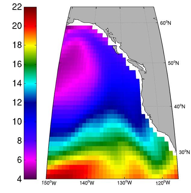
Earth System Modeling at NOAA GFDL

                                               “Atmosphere-Ocean General
                                               Circulation Models” have
                                               evolved into “Earth System
                                               Models” (ESMs) by including
                                               biosphere processes as well
                                               as physical processes.

              GFDL’s biogeochemistry model is TOPAZ and
              included major nutrient cycles (N, P, Si and Fe) and
              three phytoplankton classes.
              Dunne, et al. (2005, 2007; Global Biogeochem. Cycles)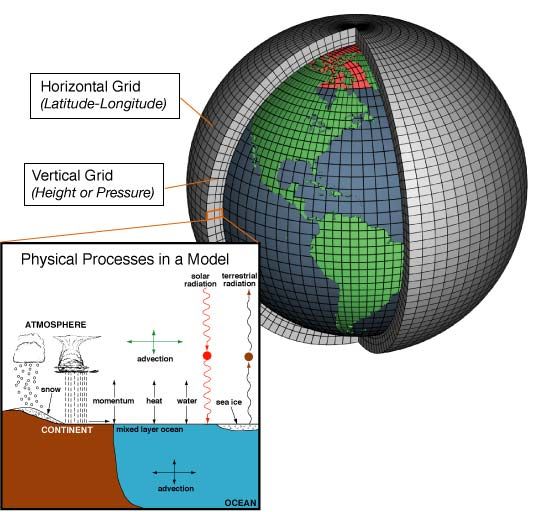
Earth System Modeling at NOAA GFDL
                                                     The coupling of these
  greenhouse-gas + natural                           models forms ESM 2.1.
  aerosol radiative forcing

                       Atmospheric model
                      AM2p12: 144 x 90 x 24

                  2o x 2.5o horizontal resolution;         Land model
                        30-min time steps                  (with biology)

            Sea-Ice             Ocean model (with biology)
            model
                                    MOM4: 360 x 200 x 50
                          1o x 1o horizontal resolution; 10-m vertical
                         resolution (in upper 200 m); 2-hr time steps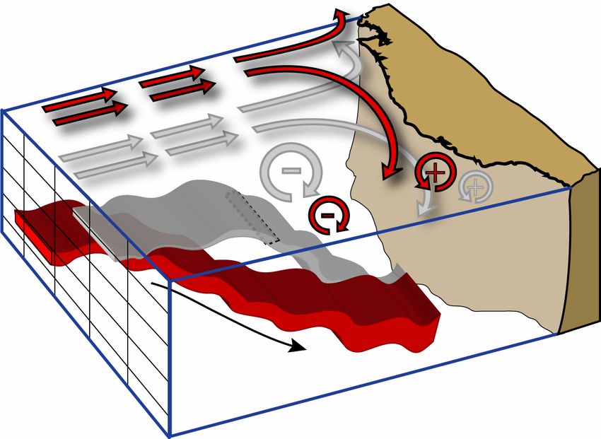
Application of Earth System Models
 Advantages
 • Major processes affecting climate included (atmosphere, ocean, land, ice, and
   biology).
 • Mathematically consistent (i.e., no observational errors).
 • No elegance required in specifying regional boundary conditions.
 Disadvantages
 • Manipulation of large model data sets requires powerful computing.

 • Incredibly complex system; difficult to trace root sources of variability.
 • Coarse resolution necessitates a focus on the regional to basin-scale.
     • Sub-grid scale processes are parameterized.
     • Coastal upwelling processes are poorly resolved.

   Question: What relatively basic, large-scale question might be addressed?

        How is nutrient supply to the California Current Ecosystem
        projected to change with global climate change?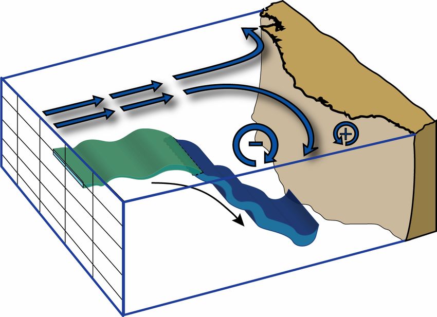
Physics affecting primary production in the CCE
 Equatorward winds driven by an atmospheric pressure gradient force
 surface waters offshore (Ekman transport) and draw nutrient-rich deep
 waters into the euphotic zone (coastal upwelling).

                                                                       alongshore,
                                                                       equatorward
                                                                          winds

                                                  offshore transport

                                                                         upwelling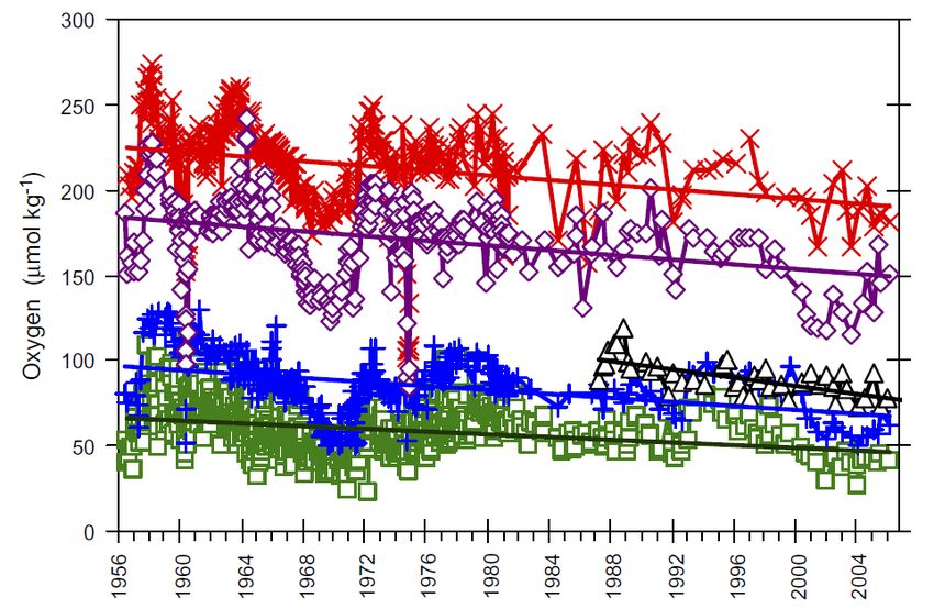
Two previous hypotheses come to mind
 #1 - Increased stratification = decreased biological production
 Roemmich and McGowan (1995) hypothesized that global warming will result in:

                              increased              reduced mixing
  increased SST              water-column            reduced efficacy of upwelling
                             stratification          reduced production

 #2 - Increased continental warming rate = increased biological production
 Bakun (1990) hypothesized that global warming will result in:

relative differences       more rapid warming            increased alongshore winds
in land and sea            over land; increased          increased upwelling
heat capacities            atm. pressure gradient        increased production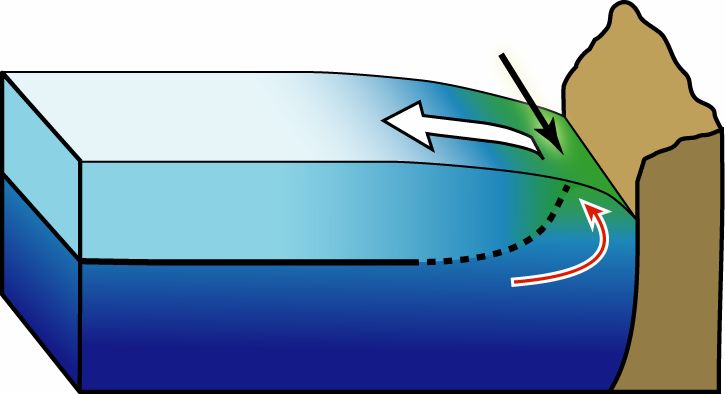
Two previous hypotheses come to mind
   #1 - Roemmich and McGowan (1995)                      #2 - Bakun (1990)
           increased stratification                      increased upwelling rate

                                                          depth
          depth

                                        (Conventional view
                  • decreased mixing    with observational        • increased vertical
                    across nutricline   support, e.g., ENSO,        transport
                  • decreased           PDO, and plain old        • increased
                    production          interannual                 production
                                        variability.)

 …Essentially, two one-dimensional models of ecosystem dynamics. Both
 are based on sound understanding of factors influencing productivity, but are
 difficult to compare quantitatively.
 At decadal scales and longer, changes in advection may be important and
 requires consideration of four dimensions. What are the model projections?
Projected changes in the North Pacific
The following plots will have four panels:
Fossil-fuel intensive
Pre-industrial mean mean Difference
(1860, 20-yr run) (SRES A2 2081-2100) (Future – pre-industrial)
PAST FUTURE DIFFERENCE
Time series for the CCE (128oW to coast, 30oN to 40oN , upper 200-m avg.)
1861 2001 2300
1860 control (pre-industrial) historical SRES A2Mean fields and long-term trends: temperature
Mean fields and long-term trends:
mixed-layer depth

    Projected responses in the CCE include a shallower mixed-layer
    depth and warmer surface layer. Given the historical record, we may
    expect decreased nutrient supply and reduced production.
Mean fields and long-term trends:
nitrate
35% decrease in the average 85% increase in average
nitrate concentration in the nitrogen concentration between
North Pacific (20° N to 65° N). 2000 and 2100 in the CCE!Mean fields and long-term trends:
wind-stress
The magnitude of upwelling-favorable winds does not change.Results of a NO3 budget analysis
A detailed budget analysis determined that the projected increase in NO3 is not
the result of:
local increased mixing
changes in local remineralization or utilization rates
riverine input
Two options remain:
A change in rate of transport of nutrient rich waters into the region.
or
A change in the NO3 concentration in the waters supplied to the region.Change in the advective supply of NO3?
from North FLUX KEY:
0.8 kmol s-1 0.3 Sv 1860, 60-yr NO3 H 2O
avg: flux flux
1.0 kmol s-1 0.2 Sv
2081-2100 NO3 H 2O
Δ = 0.1 kmol s -1
0.0 Sv avg: flux flux
change = Δ NO3 Δ H2O
from West
200 m
3.1 kmol s-1 2.4 Sv 1st column: NO3 flux
5.8 kmol s-1 3.1 Sv 2nd column: H2O flux
Δ = 2.7 kmol s-1 0.7 Sv
from Below from South
6.3 kmol s-1 0.7 Sv 0.5 kmol s-1 0.5 Sv
10 kmol s-1 0.8 Sv 1.1 kmol s-1 0.4 Sv
Δ = 4.0 kmol s-1 0.1 Sv Δ = 0.6 kmol s-1 -0.1 Sv
+ 60% + 10% Why?Results of a NO3 budget analysis
Three factors influence the nitrate concentration of a deep water mass:
1) the initial nitrate concentration of the water mass when
subducted below the ocean surface layer (i.e., “preformed”
nitrate concentration)
2) the rate of nitrate remineralization/utilization over its history
3) the length of time the water mass accrues nitrate below the
euphotic zone.History of CCE source waters
slope: accumulation rate of
remineralized NO3
intercept: initial, preformed NO3
1860 y = 0.34 x + 1.7
2081-2100 y = 0.27 x + 5.4
The projected increases in age preformed NO3 more than compensate for
reduced supply of remineralization rate (i.e., reduced surface production in
the Central North Pacific).History of CCE source waters
Locations where
deep CCE waters
are ventilated with
the surface
1860
2081-2100
Why is there this change in the trajectory and ventilation location of source
waters? Why is the transport of CCE source waters at depth prolonged?Atmospheric forcing of CCE source waters
Atmospheric forcing of CCE source waters
Atmospheric forcing of CCE source waters
 Conceptual diagram:           pre-industrial   2081-2100

                       mixed-layer

                           source-water
                             trajectory
Atmospheric forcing of CCE source waters
Conceptual diagram: pre-industrial 2081-2100
poleward shift
in westerlies
decreased
downwelling over
subtropical gyre
decreased ventilation
of source waters with
the surface source-water
trajectoryFurther implications of decreased ventilation
What do these changes in nitrate supply, oxygen, and stratification imply
for the ecosystem?
Speculation
• Increased occurrence of hypoxia and anoxia:
Decreased ventilation increases remineralized NO3 accumulation, but
decreases dissolved O2.
• Changes in nutrient stoichiometry:
Reduced NO3 supply to the subarctic N. Pacific decreases Fe limitation.
Increased NO3 supply to the CCE increases Fe limitation.Further implications of decreased ventilation
Few survey programs have been measuring NO3 or O2 long enough to
distinguish decadal variability from long-term trends.
However, those that have
examined O2 or other
biologically relevant
properties suggest
consistent long-term
trends:
Aksnes and Ohman (2009)
Whitney, et al. (2007)
Nakanowatari, et al. (2007)
Bograd, et al. (2008)
Whitney, et al. (2007, Prog. Oceanogr.)Future model improvements
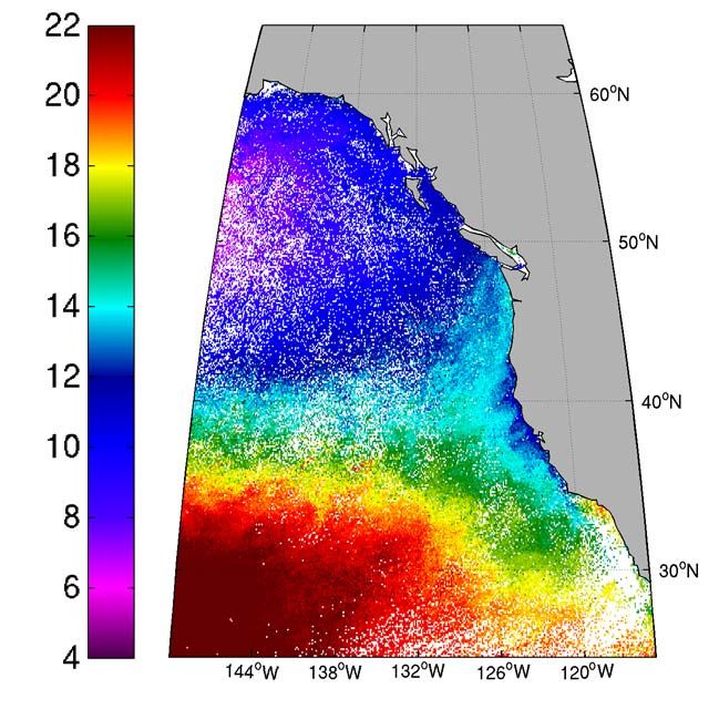
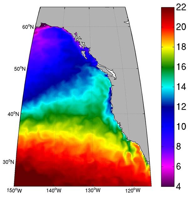
1o x 1o ocean, 2o x 2.5o atm 0.25o x 0.25o ocean, 0.5o x 0.5o atm
June SSTFuture model improvements
AVHRR, June 2010 0.25o x 0.25o ocean, 0.5o x 0.5o atm
June SST
Additionally, folks at GFDL (Bob Hallberg, et al.) are running a higher-resolution
isopycnal model to which the biochemical model will be dynamically coupled.General results
These projections of increased nitrate supply and decreased O2 with
increased greenhouse gases and the mechanism driving these changes is
the result of a detailed analysis
one very complex and very flawed global model.
(Though better than most comparable models!)
But… there are two important general messages that come out of this
modeling experiment.General results
Two important messages
1. Historic modes of interannual and decadal variability are likely to persist in
the future.
However, these familiar oscillations will exist upon centennial scale,
anthropogenically forced trends that may be more influential than the
shorter-term oscillations.General results – Trends vs. oscillations GFDL climate model ESM2.1 display variability in SST at decadal frequency in the North Pacific.
General results – Trends vs. oscillations In the coming century, SST variability is expected to be dominated by the long-term trend.
General results
 Two important messages
 1. Historic modes of interannual and decadal variability are likely to persist in
    the future.
   However, these familiar oscillations will exist upon centennial scale,
   anthropogenically forced trends that may be more influential than the
   shorter-term oscillations.
2. Long-term relationships may be counterintuitive and opposite those
observed at interannual to decadal time scales.
Just because an empirical relationship existed in the past does not mean it
will persist in the future.
Different mechanisms operate over different time scales.General results – Empirical relationships fail
Conventional view of CCE variability:
Cool Period Warm Period
replete nutrients
May not apply to
limited nutrients
The nitrate-temperature
long-term warming
high biologic production low biologic production relationship is negative over
interannual to multidecadal
periods.
However, this relationship
cannot be extended to
temp conclude that nitrate supply
[NO3] will similarly decrease with
conditions of global
warming. Time scales and
forcings are important.
ESM 2.1 projection for [NO3]
linear expectation for [NO3] given
historical temperature relationshipThanks for listening! contact me: ryan.rykaczewski@noaa.gov
Ventilation of CCE source waters
 In the future, waters follow a deeper,
 less ventilated trajectory en route to the
 CCE. Reduced ventilation of CCE
 source waters leads to an increase in
 NO3 concentration.

 Projected long-term increase in NO3 is
 not related to :

 upwelling rate

 surface mixing
History of CCE source waters

          1860
          2081-2100
History of CCE source waters
1860
2081-2100History of CCE source waters
more downwelling
less downwelling
less downwelling
more downwelling
1860
2081-2100History of CCE source waters
more downwelling
less downwelling
less downwelling
more downwelling
1860
2081-2100History of CCE source waters
more downwelling
less downwelling
less downwelling
more downwelling
1860
2081-2100History of CCE source waters
more downwelling
less downwelling
less downwelling
more downwelling
1860
2081-2100History of CCE source waters
more downwelling
less downwelling
less downwelling
more downwelling
1860
2081-2100History of CCE source waters
more downwelling
less downwelling
less downwelling
more downwelling
1860
2081-2100History of CCE source waters
more downwelling
less downwelling
less downwelling
more downwelling
1860
2081-2100History of CCE source waters
more downwelling
less downwelling
less downwelling
more downwelling
1860
2081-2100You can also read