Deep learning methodology for predicting time history of head angular kinematics from simulated crash videos
←
→
Page content transcription
If your browser does not render page correctly, please read the page content below
www.nature.com/scientificreports
OPEN Deep learning methodology
for predicting time history of head
angular kinematics from simulated
crash videos
Vikas Hasija1,3* & Erik G. Takhounts2,3
Head kinematics information is important as it is used to measure brain injury risk. Currently, head
kinematics are measured using wearable devices or instrumentation mounted on the head. This paper
evaluates the deep learning approach in predicting time history of head angular kinematics directly
from videos without any instrumentation. To prove the concept, a deep learning model was developed
for predicting time history of head angular velocities using finite element (FE) based crash simulation
videos. This FE dataset was split into training, validation, and test datasets. A combined convolutional
neural network and recurrent neural network based deep learning model was developed using the
training and validations sets. The test (unseen) dataset was used to evaluate the predictive capability
of the deep learning model. On the test dataset, correlation coefficient obtained between the actual
and predicted peak angular velocities was 0.73, 0.85, and 0.92 for X, Y, and Z components respectively.
In the United States, traumatic brain injury (TBI) is a serious public health issue. In 2014, about 2.87 million
TBI related emergency department (ED) visits, hospitalizations and deaths occurred in United S tates1. Falls
and motor vehicle crashes (MVC) were the first and second leading causes of TBI-related h ospitalizations1. The
lifetime economic cost of TBI, including direct and indirect medical costs, was estimated to be approximately
$76.5 billion (in 2010 dollars)2. Given the cost and number of TBI cases, understanding the mechanism of brain
injury and preventing them is critical. Researchers over the years have found head motion kinematics to be an
important correlate to brain injuries. Many head/brain injury metrics that have been developed such as the head
injury criterion (HIC)3, brain injury criterion (BrIC)4, rotational injury criterion (RIC)5 etc. all make use of head
motion kinematics. HIC is based on linear accelerations and is part of vehicle safety regulation6, BrIC is based
on angular velocities and RIC is based on angular accelerations. Measuring head kinematics is thus extremely
important to understand the risk of brain injury.
Deep learning is a part of machine learning based on artificial neural networks and has been shown to be
very effective in solving complex problems in the area of computer vision, natural language processing, drug
discovery, medical image analysis, etc. Recently, deep learning models were used in brain injury biomechanics
field as well. Wu et al.7 used American college football, boxing and mixed martial arts (MMA) datasets along
with lab-reconstructed National Football League impacts dataset to develop a deep learning model to predict
95th percentile max principal strain of the entire brain and the corpus callosum along with fiber strain of the
corpus callosum. Zhan et al.8 used kinematic data generated by FE simulations and those collected from on-field
football and MMA using instrumented mouthguards and developed a deep learning head model to predict the
peak maximum principal strain (MPS) of every element in the brain. Ghazi et al.9 developed a convolutional
neural network (CNN) to instantly estimate element-wise distribution of peak maximum principal strain of
the entire brain using two-dimensional images of head rotational velocity and acceleration temporal profiles
as input to CNN model. Also, Bourdet et al.10 developed a deep learning model with linear accelerations and
linear velocities from helmet tests as input to the model to predict maximum Von Mises stress within the brain.
In addition to predicting strains and stresses in the brain, deep learning models have also been developed
to detect impacts to the head in American Football. Gabler et al.11 evaluated a broad range of machine learning
(ML) models and developed a Adaboost based ML model to discriminate between head impacts and spurious
events using 6DOF head kinematic data collected from a custom-fit mouthguard sensor. More recently, Raymond
1
Bowhead (Systems & Technology), Washington, DC, USA. 2National Highway Traffic Safety Administration
(NHTSA), Washington, DC, USA. 3These authors contributed equally: Vikas Hasija and Erik G. Takhounts. *email:
vikas.hasija@dot.gov
Scientific Reports | (2022) 12:6526 | https://doi.org/10.1038/s41598-022-10480-w 1
Vol.:(0123456789)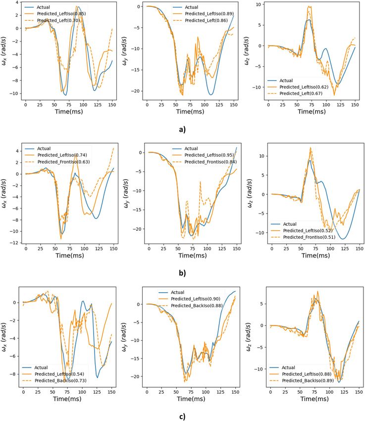
www.nature.com/scientificreports/
Figure 1. GHBMC human models in driving position (a) 5th female, (b) 50th male.
et al.12 used head kinematic data from instrumented mouthguards augmented with synthetic head kinematic data
obtained from FE head impacts to detect impacts to the head using physics-informed ML model.
One common thread in these studies is that they use head kinematics data obtained from FE simulations/
wearable devices/ head instrumentation as input for their deep learning models to predict either strains in the
brain or detect impact to the head.
Related to head kinematics, video analysis has also been used in the past. For example, Sanchez et al.13 evalu-
ated laboratory reconstruction videos of head impacts collected from professional football games. The videos
were generated from a high-speed camera recording at 500 frames per second. These videos were not used to
predict or compute head kinematics but were analyzed to identify a time region of applicability (RoA) for head
kinematics and for application to FE brain models to determine MPS and cumulative strain damage measure
(CSDM)14.
The goal of this study was to evaluate the feasibility of deep learning methodology to predict time history
of head angular kinematics directly from simulated crash videos and its applicability to controlled testing envi-
ronments like National Highway Traffic Safety Administration (NHTSA) commissioned vehicle crash tests. As
a proof of concept, a deep learning model was developed to predict time history of X, Y and Z-components of
head angular velocity vector from FE based crash videos. Angular velocity has been shown to better correlate
with brain strains as compared to angular accelerations15 and is used in brain injury criterion (BrIC) developed
by NHTSA for assessing risk of TBI. For these reasons, predicting angular velocity time histories was chosen
for this study, while corresponding angular accelerations could be readily computed from the time histories of
angular velocities. Skull fracture in not a major concern in vehicular crashes16 due to the presence of airbags and
thus linear acceleration based head injury criterion (HIC) was not considered.
Methods
Data. A supervised deep learning model takes in the inputs and the corresponding outputs and learns the
mapping between the inputs and the outputs. For developing a deep learning model for predicting time history
of angular velocities from crash videos, crash videos are required as inputs and the corresponding time history
of angular velocities are required as outputs. FE based crash simulation data was utilized in this proof of concept
study.
To generate the data, validated simplified Global Human Body Models Consortium (GHBMC) 50th percentile
male17,18 and 5th percentile female19,20 FE human models were used in a variety of frontal crash simulations.
These human models were positioned in the driver compartment (Fig. 1) that was extracted from the validated
FE model of a 2014 Honda A ccord21.
A validated generic seatbelt system with retractor, pretensioner and load limiter was included in the model
along with validated frontal and side a irbags21. In addition, steering column collapse was implemented and was
included in these simulations. The roof rails, side door, B-pillar, and floor were deformable in the full FE model,
but were made rigid in this study. The knee bolster and A-pillar were kept deformable. The human models were
positioned in the driver compartment based on clearance measurements taken from physical crash tests (NHTSA
test number 8035 for 50th male, NHTSA test number 8380 for 5th female; https://www-nrd.nhtsa.dot.gov/datab
ase/veh/veh.htm). The crash pulse used for the simulations was taken from a physical crash test (NHTSA test
number 9476) and is shown in Supplementary document Sect. 1.
These human models were evaluated in full frontal test condition, following which a design of experiments
(DOE) study was conducted. For the DOE study, both crash-related parameters and restraint-related parameters
were varied (Table 1). The crash related parameters were Delta-V and principal direction of force (PDOF). The
restraint parameters were both seatbelt and airbag related. The parameters were varied over a wide range to
generate a range of head motions including cases where the head hits the steering wheel.
The crash pulse for the same vehicle may be different for different PDOF, frontal overlap, and type and stiff-
ness of the impacting surface. In addition, for the same PDOF, frontal overlap, and impacting surface, the crash
pulse can vary for different vehicles of the same size (e.g., mid-size sedans). To keep the number of variables
manageable for the DOE study, crash pulse shape was kept constant. Only crash pulse magnitude was scaled to
achieve different Delta-Vs.
A total of 1010 scenarios were simulated covering a wide range of crash conditions. Each crash scenario was
simulated for a duration of 150 ms, which takes approximately 4.5 h on 28 processors. For each simulation, the
Scientific Reports | (2022) 12:6526 | https://doi.org/10.1038/s41598-022-10480-w 2
Vol:.(1234567890)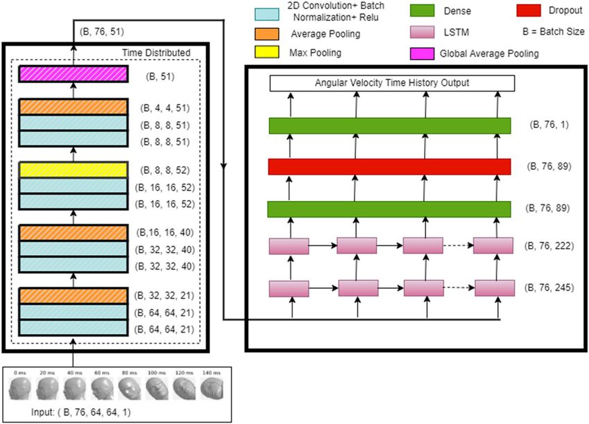
www.nature.com/scientificreports/

                                  Parameter                                     Range
                                  Crash-related parameters
                                  Delta-V                                       25–45 mph
                                  PDOF                                          − 30° (near side)–30° (far side)
                                  Restraint-related parameters
                                  Frontal & side airbag mass flow rate          ± 25%
                                  Frontal & side airbag firing time             5–70 ms
                                  Collapsible column breaking force             3000–10,000 N
                                  Load limiter                                  1000–5000 N
                                  Pretensioner limiting force                   1000–3000 N
                                  Friction between head and front/side airbag   0–3

                                 Table 1.  Parameters and their ranges.

                                 Figure 2.  (a) Head rotational axes, and (b) Views used to generate videos: left isometric, back isometric, front
                                 isometric, and left.

                                 time history of head angular velocities about the three head rotational axes (Fig. 2a) was computed and four
                                 crash videos with different views were generated (Fig. 2b).
                                     The views chosen were similar to camera views available from NHTSA crash tests. Since the aim of the study
                                 was to predict the time history of head angular velocities from any view, each crash view was treated as a separate
                                 sample. Thus, we had a total of 4040 crash videos and their corresponding head angular velocity time histories
                                 (ωx, ωy, ωz) about the three head rotational axes.
                                     The crash videos were then used as inputs for the deep learning model and the corresponding angular veloc-
                                 ity time histories were used as the “ground truth” outputs. For the purposes of this study, all crash videos were
                                 generated such that only the human model was visible. The vehicle structure and the airbags were removed from
                                 the videos to prevent any head occlusion.
                                     Since videos are used as inputs to the deep learning model in the form of sequence of images, an additional
                                 input pre-processing step was carried out to convert the FE based crash videos to sequences of RGB images.
                                 Given the goal of this study was to predict the time histories of head angular velocities, the motion of the head
                                 was extracted as a sequence of RGB images over time from each FE crash video (Supplementary document
                                 Sect. 2). These sequences of images were then used as inputs to the deep learning model.
                                     The images were extracted every 2 ms from the 150 ms crash event and thus each sequence of images had a
                                 length of 76. The corresponding “ground truth” time histories of angular velocities (outputs or targets) were also
                                 sampled every 2 ms to match the corresponding sequence of images. This was done to support the deep learning
                                 architecture used in this study as described below in the deep learning model section. An example of the input
                                 and corresponding output for training the deep learning model is shown in Fig. 3. For visualization purpose,
                                 the input sequence of images in Fig. 3 is shown every 20 ms.

Scientific Reports |   (2022) 12:6526 |                      https://doi.org/10.1038/s41598-022-10480-w                                              3

                                                                                                                                             Vol.:(0123456789)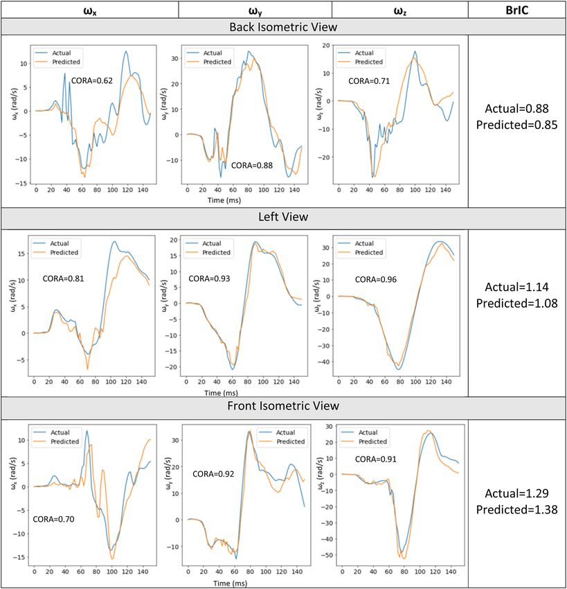
www.nature.com/scientificreports/
20
15
10
ωy (rad/s)
5
0
-5 0 40 80 120 160
-10
-15
-20
Time (ms)
a) b)
Figure 3. (a) Sample input, and (b) corresponding “ground truth” output for training.
Input data transformation. The input data (sequence of images) were RGB images with pixel values in
the range from 0 to 255. Deep learning models train better and faster when input data is on the same scale. Thus,
all the input sequences of images were normalized so that the pixel values were in the range from 0 to 1. Due
to resource limitations, all images were resized to a height and width of 64 pixels and subsequently converted
to grayscale such that each sequence of images had a shape of (76, 64, 64, 1), where number 76 stands for the
number of images in a sequence, numbers 64 are for image size, and 1 stands for the number of channels (1
represents grayscale image).
Data splitting. The entire dataset had 4040 samples. For developing the deep learning model, this dataset
was split into three datasets: training, validation and test datasets. 74% the data was used for training, 13% of
the data was used for validation and 13% of the data was used for testing. Data splitting was carried out using
stratified sampling based on human model size and the crash view to ensure each of these (human model size
and crash view) were equally represented in all three datasets (Supplementary document Sect. 3).
The training and validation datasets (87% of the data) were used for model development. The validation
dataset was used for hyperparameters tuning and was a part of model development. The test dataset was not
used in model development and was treated as an unseen dataset that was used to evaluate the final performance
of the model.
Deep learning model. The overall architecture for a deep learning model depends on the type of input
data. The input data in this study is a sequence of images over time. Convolutional neural networks (CNN)
can capture spatial dependency and are one of the most common types of neural networks used in computer
vision to recognize objects and patterns in images. On the other hand, recurrent neural networks (RNN) can
capture temporal dependency and are commonly used for sequential data processing. Thus, to process sequences
of images in this study, a deep learning model that combines CNN22 and Long Short-Term Memory (LSTM)23
based RNN was used. The CNN-LSTM architecture uses CNN layers for feature extraction on input data com-
bined with LSTMs to support sequence prediction.
Since the best architecture for our problem was not known at the start of model development, a lightweight
baseline model (with fewer trainable parameters) was developed, which was later improved using hyperparameter
tuning. For the CNN part of the baseline model, a Visual Geometry Group (VGG) style architecture24 was used,
which consisted of a three-block network with two convolutional layers per block followed by a max pooling layer.
Batch normalization25 and a rectified linear unit (ReLU) activation f unction26 were used after each convolutional
layer. The baseline (initial) values selected for the number of convolutional filters for the three blocks were 16,
32 and 64 respectively. A global average pooling layer was added as the last layer of the CNN model to obtain
the feature vector. Since each input sample is a sequence of images, the CNN part of the model was wrapped in a
time distributed layer27 to get feature vector corresponding to the entire sequence. The time distributed wrapper
helps apply the same CNN network to every temporal slice (image) of the input. The output from CNN was used
as an input to the LSTM network. The LSTM network can be set up in multiple ways, the details of which are
provided in Supplementary document Sect. 4. For the LSTM part of the baseline model, one LSTM layer with a
hidden size of 128 was used. Since input sequence has a length of 76 and the goal is to predict the time history
of angular velocity, the output was obtained at each recurring timestep from the LSTM layer. The output of the
LSTM was then used as an input for a fully-connected layer with the ReLU activation function, followed by a
dropout layer28 to control for overfitting. The output of the dropout layer was then fed to a fully-connected layer
with a linear activation function to generate the final output, i.e. the predicted time history of angular velocity.
Linear activation generates continuous numerical values and hence was used in the final output layer as angular
velocity time history prediction was solved as a regression task.
The mean squared error (MSE) between the actual and predicted time history was used as the loss function
for training the entire model. Adaptive moment estimation (Adam) optimizer29 was utilized for optimization.
Since the ReLU activation was used in the network, He-Normal initializer30 was used to initialize the trainable
weights of the model. The model was developed using Tensorflow v2.427. The training was carried out on Google
Colab using a single Tesla-P100 GPU. The model training time ranged from 1.5 to 2 h.
Individual deep learning models and training. Training a single deep learning model to predict time
history of all three components of angular velocity did not produce good results. Since the three components of
Scientific Reports | (2022) 12:6526 | https://doi.org/10.1038/s41598-022-10480-w 4
Vol:.(1234567890)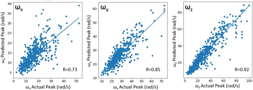
www.nature.com/scientificreports/
Figure 4. Combined deep learning model.
angular velocity (ωx, ωy, ωz) are independent of each other, three separate deep learning models were trained—
one for each component of angular velocity ωx, ωy, and ωz, which led to marked improvement in the results. The
same training and validation inputs were used for training all three models. Only the “ground truth” targets were
changed depending on the model. The baseline models for ωx, ωy, and ωz were trained with a learning rate of
0.0001 and with a batch size of 4 for a maximum of 80 epochs. Early s topping27 with a patience of 10 and model
checkpointing27 callbacks were used to save the best model based on validation loss. Models often benefit from
educeLROnPlateau27
reducing the learning rate by a factor of 2–10 once learning stagnates. For this purpose, R
callback was utilized. This callback monitors the validation loss and if no improvement is seen for 5 epochs, the
learning rate is reduced.
The hyperparameter values chosen for the CNN, LSTM, and the extended part of the baseline model were
selected at random and did not necessarily correspond to the best architecture for the problem. To improve the
models, hyperparameter tuning (Supplementary document Sect. 5) was carried out to find the set of hyperpa-
rameter values that give the best results for our problem.
Because of resource limitations, hyperparameter tuning was only performed for the ωx model to find the best
set of hyperparameters. This set of hyperparameters was then used to train the final deep learning models for
all three components of angular velocity.
Combined model. The three individually trained models for ωx, ωy, and ωz were combined into a single
deep learning model as shown in Fig. 4. To predict the time history of the three components of angular veloc-
ity from a video input of any view, the video (preprocessed as sequence of images) is passed into the combined
model. It is then propagated (forward pass) through the individually trained networks that output the time his-
tory of the three components of angular velocity ωx, ωy, and ωz.
Model evaluation. Individual model evaluation. The three individually trained deep learning models for
ωx, ωy, and ωz were evaluated on the test dataset to see how well they generalize on unseen data. The actual and
ORA31. While time
predicted time histories for cases from the test dataset were compared quantitatively using C
histories of angular velocities are important to assess overall head kinematics, for computing brain injury met-
rics peak values are usually used. For example, brain injury criterion (BrIC)4 is computed using absolute peaks
of ωx, ωy, and ωz (Eq. (1)).
ωxm
2
ωym
2
ωzm
2
BrIC = + + (1)
66.25 56.45 42.87
To evaluate prediction of the peak angular velocity, correlation coefficient between the actual and predicted
peaks was computed for all three models using the test dataset.
Frame rate evaluation. The individual models were trained on a sequence of images captured every 2 ms, i.e.
500 frames/second (fps) videos (Fig. 5a). Evaluation was carried out to determine the influence of frame rate on
both time history and peak predictions. Three different frame rates were evaluated i.e. 250 fps, 125 fps and real
time video at 25 fps. For this evaluation, the “ground truth” angular velocities sampled every 2 ms were kept the
same, but the input sequence of images were changed. For 250 fps, images sampled every 4 ms were kept in the
sequence of images while others were converted to a black image (Fig. 5b). Similarly, only images sampled at
8 ms and 40 ms were kept for 125 fps (Fig. 5c) and 25 fps (Fig. 5d) while the rest were converted to black images.
This procedure was followed to support the deep learning architecture described above.
Models were trained for ωx, ωy, and ωz for each frame rate using the same hyperparameters as in the 500 fps
study. These models were then evaluated on the test dataset by quantitatively comparing the actual and predicted
time histories using CORA for the same cases as the 500 fps study. In addition, correlation coefficients between
the actual and predicted peaks were evaluated.
Combined model evaluation. The combined model was evaluated for a few cases from the test dataset. For these
cases, the actual and predicted time histories were compared using CORA. These actual and predicted time his-
tories were also used to simulate the SIMon head m odel15 to compare the actual and predicted brain strains. In
addition, the actual and predicted BrIC values were compared.
Scientific Reports | (2022) 12:6526 | https://doi.org/10.1038/s41598-022-10480-w 5
Vol.:(0123456789)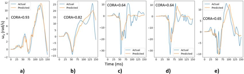
www.nature.com/scientificreports/

                                           Figure 5.  Input sequence of Images for (a) 500 fps, (b) 250 fps, (c) 125 fps, and (d) 25 fps. Image sequences
                                           shown for first 50 ms only for visualization purposes.

                                           Figure 6.  Crash pulses from NHTSA crash tests.

                                           Camera view performance evaluation. Since four different views were used in this study to train the models,
                                           evaluation was conducted using the test dataset to determine the performance of each view. For each view,
                                           average CORA scores were computed for all three components of angular velocity (ωx, ωy, and ωz). Correlation
                                           coefficients between the actual and predicted peaks for the three components of angular velocity were computed
                                           for each view as well. Both the average CORA scores and correlation coefficients were used to make the perfor-
                                           mance determination.

                                           Additional crash pulse evaluation. The models for ωx, ωy, and ωz were trained using a single crash pulse (Sup-
                                           plementary document Sect. 1), which was taken from NHTSA test 9476 (2015 Chevrolet Malibu in a frontal
                                           oblique offset test). The crash pulse magnitude was changed but shape was kept the same. To test the robust-
                                           ness, the combined model was further evaluated using three additional crash pulses (Fig. 6). These crash pulses
                                           were taken from the NHTSA test numbers 8035 (2013 Honda Accord in a frontal Impact test), 9010 (2015 Ford
                                           Escape in a frontal Impact test), and 9011 (2015 Dodge Challenger in a frontal Impact test). Frontal impacts were
                                           simulated with these additional crash pulses using the 50th male GHBMC model. Videos were then generated
                                           for these simulations and the combined deep learning model time history predictions were compared with the
                                           actual time histories of head angular velocities.

                                           Results
                                           Final model architecture. Figure 7 shows the final model architecture with tuned hyperparameters (Sup-
                                           plementary document Sect. 5, Supplementary Table S2). The data shapes shown in Fig. 7 are the output shapes
                                           from each layer. This model has approximately 845,000 trainable parameters.

                                           Model evaluation. Individual model evaluation. The final deep learning models (with tuned hyperparam-
                                           eters) for ωx, ωy, and ωz were assessed on the test dataset to evaluate how well they generalize on unseen data.
                                           Figure 8 shows the actual and predicted time histories for ωx for 5 randomly selected cases from the test dataset
                                           along with their respective CORA score. It can be observed that the ωx deep learning model is able to predict the
                                           time histories reasonably well for these cases.

          Scientific Reports |   (2022) 12:6526 |               https://doi.org/10.1038/s41598-022-10480-w                                                  6

Vol:.(1234567890)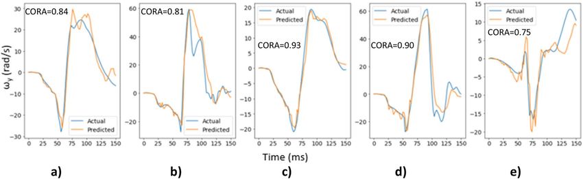
www.nature.com/scientificreports/

                                 Figure 7.  Final model architecture.

                                 Figure 8.  Actual and predicted time histories for ωx for 5 random cases from the test dataset.

                                     Figure 9 shows the actual and predicted time histories for ωy for 5 randomly selected cases from the test
                                 dataset along with their respective CORA score, which demonstrates better prediction of the time histories for
                                 ωy component than those for ωx.
                                     Similarly, Fig. 10 shows the actual and predicted time histories for ωz for 5 randomly selected cases from the
                                 test dataset along with their respective CORA score demonstrating a reasonable match between the actual and
                                 predicted time histories. Additionally, Fig. 10 shows different types of head impacts: (1) head contacts the airbag
                                 (Fig. 10a,b,d,e), and (2) head contacts the steering wheel (Fig. 10c). The model is able to predict the time history
                                 for these different head impacts demonstrating that the trained deep learning models are capable of learning
                                 important features that distinguish between different types of head impacts.
                                     The peak angular velocities were evaluated quantitatively (Fig. 11) with correlation plots using only the unseen
                                 test dataset. Correlation coefficients were 0.73 for ωx, 0.85 for ωy and 0.92 for ωz.

                                 Frame rate evaluation. Figures 8, 9, 10 and 11 above show the results obtained with 500 fps videos. The time
                                 history results for the other three frame rates (250 fps, 125 fps and 25 fps) are shown in Supplementary docu-
                                 ment Sect. 6. Table 2 shows the correlation coefficients across the different frame rates. It can be observed that at

Scientific Reports |   (2022) 12:6526 |               https://doi.org/10.1038/s41598-022-10480-w                                                    7

                                                                                                                                               Vol.:(0123456789)
www.nature.com/scientificreports/

                                           Figure 9.  Actual and predicted time histories for ωy for 5 random cases from the test dataset.

                                           Figure 10.  Actual and predicted time histories for ωz for 5 random cases from the test dataset.

                                           Figure 11.  Correlation plots for ωx, ωy, and ωz.

                                                         Correlation coefficient between actual and predicted peaks
                                            Frame rate   Angular velocity-X    Angular velocity-Y   Angular velocity-Z
                                            500 fps      0.73                  0.85                 0.92
                                            250 fps      0.68                  0.80                 0.91
                                            125 fps      0.64                  0.70                 0.83
                                            25 fps       0.00                 0.34                  0.49

                                           Table 2.  Correlation coefficients for different frame rates.

          Scientific Reports |   (2022) 12:6526 |                https://doi.org/10.1038/s41598-022-10480-w                                   8

Vol:.(1234567890)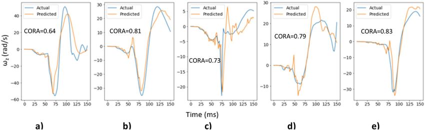
www.nature.com/scientificreports/
Figure 12. Combined model results.
250 fps, the CORA scores and correlation coefficients drop slightly compared to 500 fps results, but the results
are affected more at lower frame rates with poor predictions and correlations at 25 fps (real time videos). This is
expected as crash events last ~ 150 ms and high speed videos are necessary to capture head kinematics.
Combined model evaluation. The combined model performance was also assessed on the test dataset. Three
random videos with different views (back isometric view, front isometric view and left view) were selected from
the test dataset and the 3D angular kinematics predicted by the combined model were compared with the actual
data. The actual and predicted time history results for these three videos along with their respective CORA score
are shown in Fig. 12. The actual and predicted BrIC values are also included in Fig. 12.
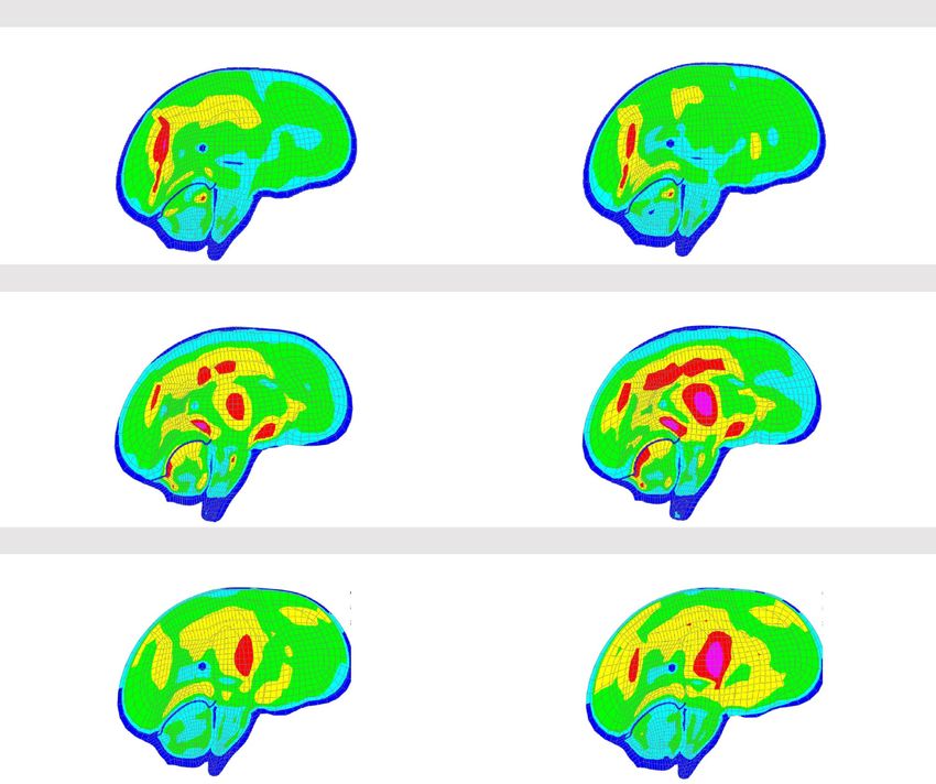
The actual and predicted time histories from the three cases (Fig. 12) were applied to the SIMon head model
to compare the brain strains. Similar actual and predicted brain strain patterns were observed for the three cases
(Fig. 13). MPS and CSDM (0.25) values were computed and are also given in Fig. 13.
Scientific Reports | (2022) 12:6526 | https://doi.org/10.1038/s41598-022-10480-w 9
Vol.:(0123456789)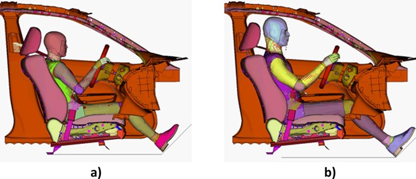
www.nature.com/scientificreports/
Actual P redicted
Back Isometric View
MPS = 0.64, CSDM = 0.27 MPS = 0.63, CSDM = 0.26
Le View
MPS = 0.79, CSDM = 0.44 MPS = 0.75, CSDM = 0.37
Front Isometric View
MPS = 1.12, CSDM = 0.80 MPS = 1.18, CSDM = 0.85
Figure 13. Brain strain comparison.
Camera view performance evaluation. The four camera views used in this study were evaluated on test dataset
to determine the view with best predictions. Figure 14 shows the average CORA scores for ωx, ωy, and ωz for each
view. An overall average CORA score (average of averages) across the three angular velocities was computed for
all four views. The left and left isometric views showed the best overall average CORA score (~ 0.73) followed by
back isometric and front isometric views (~ 0.70).
Table 3 shows the correlation coefficients between actual and predicted angular velocity peaks for the four
views. Average correlation coefficient across the three angular velocities was computed for all four views. Based
on this average score, the left isometric view showed the best results (0.88), followed by left view (0.84), back
isometric view (0.82) and finally front isometric view (0.79).
Based on CORA scores (which considers various aspects of the time history signal, such as size, shape, and
phase31) and correlation coefficients (based on peaks in this study and important for injury metric computation),
left isometric view demonstrates the best performance.
Additional crash pulse evaluation. Comparison between actual and predicted angular velocity time histories
for simulated crash videos based on crash pulses taken from NHTSA crash tests 8035, 9010 and 9011 is shown
in Fig. 15. Results are presented from two different views with their respective CORA score shown in parenthe-
ses. For all cases, results from left isometric view are presented (as it showed the best performance (Fig. 14 and
Table 3)) along with a different second view. The model shows promising predictions for all three angular veloci-
ties on these out of sample (unseen) crash videos.
Scientific Reports | (2022) 12:6526 | https://doi.org/10.1038/s41598-022-10480-w 10
Vol:.(1234567890)www.nature.com/scientificreports/
Figure 14. Average CORA scores for each camera view.
Correlation coefficient between actual and predicted peaks
Camera view Angular velocity-X Angular velocity-Y Angular velocity-Z Average correlation coefficient
Left 0.71 0.89 0.93 0.84
Back isometric 0.71 0.84 0.90 0.82
Left isometric 0.79 0.91 0.93 0.88
Front isometric 0.70 0.75 0.93 0.79
Table 3. Correlation coefficients for different camera views.
Discussion
The objective of this study was to evaluate the feasibility of deep learning methodology for predicting head
angular kinematics directly from simulated crash videos. The methodology was demonstrated by developing a
proof of concept model using FE data for predicting angular velocity time history.
Main findings. Deep learning models are function approximators that approximate the unknown underly-
ing mapping function from inputs to outputs. The results of this study show that deep learning models for ωx,
ωy, and ωz are capable of effectively capturing important features from the input sequence of images and map-
ping them to the output angular velocities, thus demonstrating the feasibility of the deep learning approach for
predicting angular head kinematics.
The deep learning models showed promising results when evaluated on the test dataset (Figs. 8, 9, 10, 11 and
12), and additional crash pulse dataset (Fig. 15) demonstrating their ability to generalize well on unseen data.
The SIMon head model simulations with three different actual and predicted angular velocity time histories
showed comparable MPS, CSDM, and brain strain patterns (Fig. 13). The actual and predicted BrIC values were
also similar for these cases (Fig. 12).
Deep learning models have been shown to work well on unstructured data, such as images, videos, text etc.
Depending on the task, deep learning models can have a large number of trainable parameters (tens of mil-
lions) and are thus trained on large datasets to avoid overfitting. For example, image classification models are
trained using the popular ImageNet dataset that has millions of images. Biomechanical datasets are very limited
for example, Wu et al.7 used a dataset of size 3069 to develop a deep learning model for efficient estimation of
regional brain strains and Zhan et al.8 used data from 1803 head impacts for developing their deep learning
model for estimation of entire brain deformation in concussion. In this study, the data size was 4040, which was
generated using 1010 FE simulations. Since dataset size is small, in addition to using regularization techniques
like dropout to avoid overfitting, the number of trainable parameters were also kept under check. The final deep
learning model had approximately ~ 845 K trainable parameters. Despite using this rather small dataset, the deep
learning models for ωx, ωy, and ωz were capable of predicting the time histories and their respective peaks well
(Figs. 8, 9, 10 and 11). This demonstrates that deep learning methodology may be feasible with small datasets,
while more data could possibly lead to better predictive models.
Scientific Reports | (2022) 12:6526 | https://doi.org/10.1038/s41598-022-10480-w 11
Vol.:(0123456789)www.nature.com/scientificreports/
Figure 15. Angular velocity time history comparison: (a) left and left isometric views (Crash pulse—NHTSA
test 8035), (b) left isometric and front isometric views (Crash pulse—NHTSA test 9010), and (c) left isometric
and back isometric views (Crash pulse—NHTSA test 9011).
The 4040 data points used in this study come from 1010 different FE simulations. The four views generated per
simulation were used as separate inputs that were not combined into one input. Combining the four views into
a single sample would require the availability of those four views for every prediction and that might become a
bottleneck if certain views are not available. The methodology used herein—treating each view as a separate input
provides the advantage of predicting kinematics from any available view that model is trained on. In addition,
the deep learning methodology does not need multiple views to get 3D kinematics and provides the advantage
of obtaining 3D kinematics from any 2D view as shown in Fig. 12.
Scientific Reports | (2022) 12:6526 | https://doi.org/10.1038/s41598-022-10480-w 12
Vol:.(1234567890)www.nature.com/scientificreports/
We used a deep learning approach to predict head angular kinematics from crash events that last ~ 150 ms. To
predict angular velocity time history from events that have similar duration, high speed cameras are preferred
for better accuracy (Figs. 8, 9 and 10, Table 2, Supplementary document Sect. 6). For short duration dynamic
events, such as a car crash, it is difficult to predict the time history using frames of images spaced out by 40 ms
(real time videos at 25 fps) as compared to predicting the time history using frames of images that are 2 ms apart
(high speed camera at 500 fps). The higher the frame rate, the better the time history predictions for the short
duration events. This may also be due to insufficient sample size when sampling a short event with lower frame
rate. The longer events (greater than 150 ms) at low frame rates were not evaluated in this study. The results
(Figs. 8, 9 and 10, Table 2, Supplementary document Sect. 6) show that high speed cameras processing at or
above 250 fps provide reasonable results for 150 ms events.
The x-component of the angular velocity vector (ωx) showed lower CORA scores (Fig. 14) and had more
discrepancy in predicting peak values (Fig. 11) when compared to ωy, and ωz. The reason for this discrepancy
may be due to the views (left, left isometric, front isometric and back isometric) selected for training the models.
These views may be more conducive for learning important features related to prediction of ωy, and ωz, but not
so much for ωx. Based on CORA scores and correlation coefficients (Fig. 14, Table 3), the best camera view for
ωx, and ωy was the left isometric view. For ωz, left, left isometric, and front isometric views provided equally good
results. Overall, left isometric camera view demonstrated best performance.
The deep learning methodology shows promising results even with low resolution (64,64) grayscale images
and limited hyperparameter tuning. Given enough resources, better models may be developed for real world
applications by using this methodology with higher resolution RGB images, exploring a wider range of hyper-
parameters and using more advanced CNN architectures like Residual n etworks32, EfficientNets33 etc. that may
help the networks learn better features from the input sequence of images, thus further improving predictions.
Applicability to NHTSA crash tests. The methodology in this study demonstrated good results in a
controlled FE environment where the head characteristics are the same for all data samples, similar camera
angles are available, and unobstructed view is available for the duration of the crash event. Thus, this methodol-
ogy holds promise for real-world controlled environment applications, for example testing environments like
NHTSA crash tests where anthropomorphic test devices (ATDs) have similar head characteristics, fixed camera
angles are available and unobstructed view is available from a back camera. Predictive models, once developed
using this deep learning methodology, from NHTSA crash test data may be used to obtain head 3D rotational
kinematics from the crash test videos involving 5th percentile ATD, which have limited head instrumentation
and currently don’t have sensors to output rotational head kinematics.
Comparison with other related work. We used a deep learning architecture that combines CNN and
LSTM to capture spatial and temporal dependency respectively. A sequence of 2D head images served as an
input while the time history of head angular velocity was the model output. Various deep learning architectures
have been used in brain injury biomechanics field. For example, Wu et al.7 used a CNN architecture to predict
regional brain strain by using 2D images of the head angular kinematics profiles as input. Similarly, Ghazi et al.9
applied CNN model to estimate element-wise strain in the brain by using 2D images of rotational velocity and
acceleration 2D profiles. In both studies, the input was a single image (not a sequence of images) and the output
was not the time history profile and thus they did not require use of LSTMs. Bourdet et al.10 used a U-Net style
architecture34 with 1D convolutions to output the time history of the maximum Von Mises stress in the entire
brain using time history of three linear accelerations and three angular velocities as an input. U-Net architectures
are fully convolutional networks that were developed for biomedical image segmentation. Since U-Net architec-
ture generates output with the same spatial dimension as the input because of its encoder-decoder structure, it
was not feasible for our 2D image dataset as the goal of our study was to extract feature vectors from the sequence
of 2D images for time history prediction.
Limitations. Deep learning methodology has many advantages, but it is not without limitations. For exam-
ple, the proof of concept model developed in this study cannot be directly applied to real world scenarios (for
example, NHTSA physical crash tests with ATDs) because the features learned by the model are from GHBMC
human head model and may not be directly applicable to other images, such as other human heads/models or
ATD head. However, the methodology described herein may be extended to build predictive models for such
real-world scenarios. We developed the deep learning models from FE crash videos with an unobstructed view
of the head. Head occlusion can lead to head features that may not be correctly identified, which would give
inaccurate prediction of angular velocities. For real-world data, the head may get obstructed at some point in the
event in some camera views. Thus, it is recommended to develop predictive models for real world applications
using data from camera angles in which the head remains visible (or partially visible) throughout the event. In
addition, deep learning models work well with the type of data they are trained on (i.e. deep learning models
may not be well suited for extrapolation). For example, models trained on just the front views cannot be expected
to make correct predictions based on back view videos. Thus, when making predictions, videos from camera
angles similar to those used in the model training may be necessary. This kind of limitation has also been pointed
out by Bourdet et al.10 and Ghazi et al.9 for their models.
Advantages of deep learning approach. Training deep learning models require high end machines
with GPUs. However, once trained such models can be used to make angular velocity predictions in a few mil-
liseconds from a given crash video. The inference (prediction) time for the combined model in this study was
Scientific Reports | (2022) 12:6526 | https://doi.org/10.1038/s41598-022-10480-w 13
Vol.:(0123456789)www.nature.com/scientificreports/
117 ms on a GPU. The advantage of deep learning approach is that with the availability of new data, the training
dataset may be appended for retraining, thus allowing for iterative improvement of the model.
While we developed deep learning models for predicting angular velocity time histories, the approach is not
limited to angular velocities. It may be used for predicting other kinematic parameters, such as linear accelera-
tions and linear acceleration based head injury criterion (HIC) etc.
Predicting head kinematics using deep learning methodology provides an alternative method of computing
head kinematics and may be deployed in situations where the sensor data is either not available or insufficient
to determine head angular kinematics (assuming that videos of such events are available).
Conclusions
Proof-of-concept deep learning models developed in this study showed promising results for predicting angular
velocity time histories, thus demonstrating the feasibility of deep learning methodology.
Future work. Future work involves extending this deep learning methodology to NHTSA crash tests for
predicting ATD head angular kinematics.
Received: 15 November 2021; Accepted: 30 March 2022
References
1. Surveillance Report of Traumatic Brain Injury-related Emergency Department Visits, Hospitalizations, and Deaths—United States,
2014, Centers for Disease Control and Prevention. U.S. Department of Health and Human Services (2019).
2. Finkelstein, E. et al. The Incidence and Economic Burden of Injuries in the United States (Oxford University Press, 2006).
3. Eppinger, R. et al. Development of Improved Injury Criteria for the Assessment of Advanced Automotive Restraint Systems—II,
National Highway Traffic Safety Administration (1999).
4. Takhounts, E. G., Hasija, V., Craig, M. J., Moorhouse, K. & McFadden, J. Development of brain injury criteria (Br IC). Stapp Car
Crash J. 57, 243–266 (2013).
5. Kimpara, H. & Iwamoto, M. Mild traumatic brain injury predictors based on angular accelerations during impacts. Ann. Biomed.
Eng. 40, 114–126 (2012).
6. Title 49 Code of Federal Regulations (CFR) Part571 Section 208, Occupant Crash Protection, National Highway Traffic Safety
Administration, Washington, DC: Office of the Federal Register, National Archives and Records Administration.
7. Wu, S., Zhao, W., Ghazi, K. & Ji, S. Convolutional neural network for efficient estimation of regional brain strains. Sci. Rep. https://
doi.org/10.1038/s41598-019-53551-1 (2019).
8. Zhan, X. et al. Deep learning head model for real-time estimation of entire brain deformation in concussion. arXiv:2010.08527
(2020).
9. Ghazi, K., Wu, S., Zhao, W. & Ji, S. Instantaneous whole-brain strain estimation in dynamic head impact. J. Neurotrauma 38(8),
1023–1035 (2021).
10. Bourdet, N. et al. Deep learning methods applied to the assessment of brain injury risk. In Proceedings of International Research
Conference on the Biomechanics of Impacts, Online Virtual Conference, p. IRC-21–81 (2021).
11. Gabler, L. F. et al. On-field performance of an instrumented mouthguard for detecting head impacts in American football. Ann.
Biomed. Eng. 48(11), 2599–2612 (2020).
12. Raymond, S. J. et al. Physics-informed machine learning improves detection of head impacts. arXiv:2108.08797 (2021).
13. Sanchez, E. J. et al. A reanalysis of football impact reconstructions for head kinematics and finite element modeling. Clin. Biomech.
64, 82–89 (2019).
14. Takhounts, E. G. et al. On the development of the SIMon finite element head model. Stapp Car Crash J. 47, 107–133 (2003).
15. Takhounts, E. G. et al. Investigation of traumatic brain injuries using the next generation of simulated injury monitor (SIMon)
finite element head model. Stapp Car Crash J. 52, 1–32 (2008).
16. Forman, J. et al. Automobile injury trends in the contemporary fleet: Belted occupants in frontal collisions. Traffic Inj. Prev. 20(6),
607–612 (2019).
17. Global Human Body Modeling Consortium (GHBMC), M50-OS, v2.2, (2019).
18. Schwartz, D., Guleyupoglu, B., Koya, B., Stitzel, J. D. & Gayzik, S. Development of a computationally efficient full human body
finite element model. Traffic Inj. Prev. 16, S49–S56 (2015).
19. Global Human Body Modeling Consortium (GHBMC), M05-OS, v2.2, (2019).
20. Davis, M. L., Koya, B., Schap, J. M. & Gayzik, S. Development and full body validation of a 5th Percentile female finite element
model. Stapp Car Crash J. 60, 509–544 (2016).
21. Singh, H., Ganesan, V., Davies, J., Paramasuwom, M. & Gradischnig, L. Vehicle interior and restraints modeling development
of full vehicle finite element model including vehicle interior and occupant restraints systems for occupant safety analysis using
THOR dummies. Washington, DC: National Highway Traffic Safety Administration, Report No. DOT HS 812 545. https://www.
nhtsa.gov/sites/nhtsa.gov/files/documents/812545_edagvehicleinteriorandrestraintsmodelingreport.pdf (2018).
22. LeCun, Y. & Bengio, Y. Convolutional networks for images, speech, and time series. in The Handbook of Brain Theory and Neural
Networks (Second ed.) 276–278 (The MIT press, 1995).
23. Hochreiter, S. & Schmidhuber, J. Long short-term memory. Neural Comput. 9(8), 1735–1780 (1997).
24. Simonyan, K. & Zisserman, A. Very Deep Convolutional Networks for Large-Scale Image Recognition. In International Conference
on Learning Representations (2015).
25. Loffe, S. & Szegedy, C. Batch normalization: accelerating deep network training by reducing internal covariate shift. arXiv:1502.
03167 (2015).
26. Krizhevsky, A., Sutskever, I. & Hinton, G. E. ImageNet classification with deep convolutional neural networks. Adv. Neural Inf.
Process. Syst. (2012).
27. Abadi, M. et al. TensorFlow: Large-scale machine learning on heterogeneous systems (2015).
28. Srivastava, N., Hinton, G., Krizhevsky, A., Sutskever, I. & Salakhutdinov, R. Dropout: A simple way to prevent neural networks
form overfitting. J. Mach. Learn. Res. 15, 1929–1958 (2014).
29. Kingma, D. P. & Ba, J. Adam: a method for stochastic optimization. arXiv:1412.6980 (2017).
30. He, K., Zhang, X., Ren, S. & Sun, J. Delving deep into rectifiers: surpassing human-level performance on imagenet classification.
arXiv:1502.01852 (2015).
Scientific Reports | (2022) 12:6526 | https://doi.org/10.1038/s41598-022-10480-w 14
Vol:.(1234567890)www.nature.com/scientificreports/
31. Gehre, C., Gades, H. & Wernicke, P. Objective rating of signals using test and simulation responses. In Enhanced Safety of Vehicles
(2009).
32. He, K., Zhang, X., Ren, S. & Sun, J. Deep residual learning for image recognition. In IEEE Conference on Computer Vision and
Pattern Recognition (2016).
33. Tan, M. & Le, Q. V. EfficientNet: rethinking model scaling for convolutional neural networks. arXiv:1905.11946 (2020).
34. Ronneberger, O., Fischer, P. & Brox, T. U-Net: convolutional networks for biomedical image segmentation. In Medical Image
Computing and Computer-Assisted Intervention (2015).
Disclaimer
The opinions, findings, and conclusions expressed in this publication are those of the authors and not neces-
sarily those of the Department of Transportation or the National Highway Traffic Safety Administration. The
United States Government assumes no liability for its contents or use thereof. If trade or manufacturers’ names
are mentioned, it is only because they are considered essential to the object of the publication and should not
be construed as an endorsement. The United States Government does not endorse products or manufacturers
Author contributions
V.H. conception, data generation, data preparation, data analysis, deep learning model development and training,
writing, editing; E.T. conception, writing, editing.
Competing interests
The authors declare no competing interests.
Additional information
Supplementary Information The online version contains supplementary material available at https://doi.org/
10.1038/s41598-022-10480-w.
Correspondence and requests for materials should be addressed to V.H.
Reprints and permissions information is available at www.nature.com/reprints.
Publisher’s note Springer Nature remains neutral with regard to jurisdictional claims in published maps and
institutional affiliations.
Open Access This article is licensed under a Creative Commons Attribution 4.0 International
License, which permits use, sharing, adaptation, distribution and reproduction in any medium or
format, as long as you give appropriate credit to the original author(s) and the source, provide a link to the
Creative Commons licence, and indicate if changes were made. The images or other third party material in this
article are included in the article’s Creative Commons licence, unless indicated otherwise in a credit line to the
material. If material is not included in the article’s Creative Commons licence and your intended use is not
permitted by statutory regulation or exceeds the permitted use, you will need to obtain permission directly from
the copyright holder. To view a copy of this licence, visit http://creativecommons.org/licenses/by/4.0/.
© The Author(s) 2022
Scientific Reports | (2022) 12:6526 | https://doi.org/10.1038/s41598-022-10480-w 15
Vol.:(0123456789)You can also read