Deep transfer learning for image classification: a survey - arXiv
←
→
Page content transcription
If your browser does not render page correctly, please read the page content below
Deep transfer learning for image classification: a survey
                                                                             Jo Plested1* and Tom Gedeon2
arXiv:2205.09904v1 [cs.CV] 20 May 2022

                                             1* Schoolof Engineering and Information Technology, University of New South Wales,
                                                               Northcott Drive, Campbell, 2612, ACT, Australia.
                                             2 Optus Centre for Artificial Intelligence, Curtin University, Kent Street, Bentley, 6102,

                                                                                    WA, Australia.

                                                            *Corresponding author(s). E-mail(s): j.plested@unsw.edu.au;
                                                                 Contributing authors: tom.gedeon@curtin.edu.au;

                                                                                            Abstract
                                              Deep neural networks such as convolutional neural networks (CNNs) and transformers have achieved
                                              many successes in image classification in recent years. It has been consistently demonstrated that best
                                              practice for image classification is when large deep models can be trained on abundant labelled data.
                                              However there are many real world scenarios where the requirement for large amounts of training
                                              data to get the best performance cannot be met. In these scenarios transfer learning can help improve
                                              performance. To date there have been no surveys that comprehensively review deep transfer learning
                                              as it relates to image classification overall. However, several recent general surveys of deep transfer
                                              learning and ones that relate to particular specialised target image classification tasks have been
                                              published. We believe it is important for the future progress in the field that all current knowledge
                                              is collated and the overarching patterns analysed and discussed. In this survey we formally define
                                              deep transfer learning and the problem it attempts to solve in relation to image classification. We
                                              survey the current state of the field and identify where recent progress has been made. We show
                                              where the gaps in current knowledge are and make suggestions for how to progress the field to fill
                                              in these knowledge gaps. We present a new taxonomy of the applications of transfer learning for
                                              image classification. This taxonomy makes it easier to see overarching patterns of where transfer
                                              learning has been effective and, where it has failed to fulfill its potential. This also allows us to
                                              suggest where the problems lie and how it could be used more effectively. We demonstrate that
                                              under this new taxonomy, many of the applications where transfer learning has been shown to be
                                              ineffective or even hinder performance are to be expected when taking into account the source and
                                              target datasets and the techniques used. In many of these cases, the key problem is that methods and
                                              hyperparameter settings designed for large and very similar target datasets are used for smaller and
                                              much less similar target datasets. We identify alternative choices that could lead to better outcomes.

                                              Keywords: Deep Transfer Learning, Image Classification, Convolutional Neural Networks, Deep Learning

                                         1 Introduction                                             recently transformers have achieved many suc-
                                                                                                    cesses in image classification [26, 58, 62, 73, 74].
                                         Deep neural network architectures such as con-             It has been consistently demonstrated that these
                                         volutional neural networks (CNNs) and more                 models perform best when there is abundant

                                                                  1
labelled data available for the task and large mod- make suggestions for how to progress the field to
els can be trained [50, 70, 87]. However there are fill in these knowledge gaps. While there are many
many real world scenarios where the requirement surveys in related domains and specific sub areas,
for large amounts of training data cannot be met. to the best of our knowledge there are none that
Some of these are: focus on deep transfer learning for image classifi-
cation in general. We believe it is important for the
1. Insufficient data because the data is very rare
future progress in the field that all the knowledge
or there are issues with privacy etc. For exam-
is collated together and the overarching patterns
ple new and rare disease diagnosis tasks in the
analysed and discussed.
medical domain have limited training data due
We make the following contributions:
to both the examples themselves being rare and
privacy concerns. 1. formally defining deep transfer learning and the
2. It is prohibitively expensive to collect and/or problem it attempts to solve as it relates to
label data. For example labelling can only be image classification
done by highly qualified experts in the field. 2. performing a thorough review of recent
3. The long tail distribution where a small number progress in the field
of objects/words/classes are very frequent and 3. presenting a taxonomy of source and target
thus easy to model, while many many more are dataset relationships in transfer learning appli-
rare and thus hard to model [6]. For example cations that helps highlight why transfer learn-
most language generation problems. ing does not perform as expected in certain
application areas
There are a several other reasons why we may
4. giving a detailed summary of source and tar-
want to learn from a small number of training
get datasets commonly used in the area to
examples:
provide an easy reference for the reader look-
• It is interesting from a cognitive science per- ing to understand relationships between where
spective to attempt to mimic the human ability transfer learning has performed best and where
to learn general concepts from a small number results have been less consistent
of examples. 5. summarizing current knowledge in the area
• There may be restraints on compute resources as well as pointing out knowledge gaps and
that limit training a large model from random suggested directions for future research.
initialisation with large amounts of data. For
In Section 2 we review all surveys in the area
example environmental concerns [124].
from general transfer learning, to more closely
In all these scenarios transfer learning can often related domains. In section 3 we introduce the
greatly improve performance. In this paradigm the problem domain and formalise the difficulties with
model is trained on a related dataset and task learning from small datasets that transfer learning
for which more data is available and the trained attempts to solve. This section includes termi-
weights are used to initialise a model for the target nology and definitions that are used throughout
task. In order for this process to improve rather this paper. Section 4 details the source and tar-
than harm performance the dataset must related get datasets commonly used in deep learning for
closely enough and best practice methods used. image classification. Section 5 provides a detailed
In this survey we review recent progress in deep analysis of all recent advances and improvements
transfer learning for image classification and high- to transfer learning and specific application areas
light areas where knowledge is lacking and could and highlights gaps in current knowledge. In
be improved. With the exponentially increasing Section 6 we give an overview of other problem
demand for the application of modern deep CNN domains that are closely related to deep transfer
models to a wider array of real world application learning for image classification including the sim-
areas, work in transfer learning has increased at ilarities and differences in each. Finally Section 7
a commensurable pace. It is important to regu- summarises all current knowledge, gaps and prob-
larly take stock and survey the current state of the lems and recommends directions for future work
field, where recent progress has been made and in the area.
where the gaps in current knowledge are. We also
22 Related work learning and image classification the trends in this
area are not covered.
Many reviews related to deep transfer learning Weiss et al. [141] divide general transfer learn-
have been published in the past decade and the ing into homogeneous, where the source and target
pace has only increased in the last few years. How- dataset distributions are the same, and heteroge-
ever, they differ from ours in two main ways. The neous, where they are not, and give a thorough
first group consists of more general reviews, that description of each. They review many different
provide a high level overview of transfer learning approaches in each category, but few of them are
and attempt to include all machine learning sub- related to deep neural networks.
fields and all task sub-fields. Reviews in this group
are covered in Section 2.1. The second group is
2.2 Closely related work
more specific with reviews providing a compre-
hensive breakdown of the progress on a particular There are some recent review papers that based on
narrow domain specific task. They are discussed their title seem to be more closely related. How-
in the relevant parts of Section 5.7. There are a ever, they are short summary papers containing
few surveys that are more closely related to ours limited details on the subject matter rather than
with differences discussed in Section 2.2. full review papers.
A Survey on Deep Transfer Learning [127]
2.1 General transfer learning defines deep transfer learning and separates it into
four categories based on the subset of techniques
surveys
used. The focus is more on showing a broad selec-
The most recent general transfer learning sur- tion of methods rather than providing much detail
vey [46], is an extremely broad overview of most or focusing particularly on deep transfer learning
areas related to deep transfer learning including methods. Most major works in the area from the
those areas related to deep transfer learning for past decade are missing.
image classification outlined in Section 6. As it is a Deep Learning and Transfer Learning
broad general survey there is no emphasis on how Approaches for Image Classification [56] focuses
deep transfer learning applies to image classifica- on defining CNNs along with some of the major
tion and thus the trends seen in this area are not architectures and results from the past decade.
covered. The paper includes a few brief paragraphs defin-
A thorough theoretical analysis of general ing transfer learning and some of the image
transfer learning techniques is given in [158]. classification results incorporate transfer learning,
Transfer learning techniques are split into data- but no review of the topic is performed.
based and model-based, then further divided into A Survey of Transfer Learning for Convolu-
subcategories. Deep learning models are explicitly tional Neural Networks [106] is a short paper
discussed as a sub-Section of model-based cate- which briefly introduces the transfer learning task
gorisation. The focus is on generative models such and settings, and introduces general categories of
as auto-encoders and Generative Adversarial Net- approaches and applications. It does not review
works (GANs) and several papers are reviewed. any specific approaches or applications.
Neural networks are also mentioned briefly under Transfer Learning for Visual Categorization: A
the Parameter Control Strategy and Feature Survey [115]. Is a full review paper, but is older
Transformation Strategy Sections. However, the with no deep learning techniques included.
focus is on unsupervised pretraining strategies, In Small Sample Learning in Big Data Era
rather than best practice for transferring learning. [119] deep transfer learning is a large part of the
Zhang et al. [153] take the most similar work, but not the focus. Some examples of deep
approach to categorizing the transfer learning task learning applied to image classification domains
space as ours. They divide transfer learning into are mentioned, but there is no discussion of meth-
17 categories based on source and target dataset ods for improving deep transfer learning as it
and label attributes. They then review approaches relates to image classification.
taken within each category. Since it is a general
transfer learning survey with no focus on deep
33 Overview [41], in practice because the loss function is non-
convex with respect to the weights it is difficult
3.1 Problem Definition to optimise. For this reason modern networks are
In this Section definitions used throughout the often arranged in very deep networks and task spe-
paper are introduced. Transfer learning can be cific architectures, like CNNs and transformers for
categorised by both the task and the mode. We images, to allow for easier training of parameters.
start by defining the model, then the task and The hierarchical structure of these networks
finally how they interact together in this case. allows for ever more complex patterns to be
Deep learning is a modern name for neural learned. This is one of the things that has allowed
networks with more than one hidden layer. Neu- deep learning to be successful at many different
ral networks are themselves a sub-area of machine tasks in recent years, when compared to other
learning. Mitchell [79] provides a succinct defini- machine learning algorithms. However, this only
tion of machine learning: applies if there is enough data to train them.
Figure 1 shows the increase in ImageNet 1K per-
formance with the number of model parameters.
Definition 1 ”A computer program is said to learn Figure 2 shows that for large modern CNN mod-
from experience E with respect to some class of tasks els in general the performance on ImageNet 1K
T and performance measure P, if its performance at
increases with the number of training examples in
tasks in T, as measured by P, improves with experience
the source dataset. This suggests that large mod-
E.”
ern CNNS are likely overfitting when trained from
random initialization on ImageNet 1K. Of course
Neural networks are defined by Gurney [33] as: there are some outliers as the increase in perfor-
mance from additional source data also depends
Definition 2 ”A neural network is an intercon- on how related the source data is to the target
nected assembly of simple processing elements, units data. This is discussed further in in Section 5.3.1.
or nodes, called neurons, whose functionality is loosely These two results combine to show the stated
based on the animal neuron. The processing ability effect that deep learning performance scales with
of the network is stored in the inter unit connec- the size of the dataset and model.
tion strengths, or weights, obtained by a process of As noted in section 1 there are many real world
adaptation to, or learning from, a set of training scenarios where large amounts of data are unavail-
patterns.”
able or we are interested in training a model on a
small amount of data for other reasons.
The neurons in a multilayer feed forward neu-
ral network of the type that we consider in this 3.2 Learning from small vs large
review have nonlinear activation functions [29] and datasets
are arranged in layers with weights W feeding
forward from one layer to the next. A thorough review of the problems of learning
Generally, a neural network learns to improve from a small number of training examples is given
its performance at task T from Experience E, in [139].
being the set of training patterns, via gradient
descent and backpropagation. Backpropagation is 3.2.1 Empirical Risk Minimization
an application of the chain rule applied to prop- We are interested in finding a function f that
agate derivatives from final layers of the neural minimises the expected risk:
network to the hidden and input weights [110].
There are other less frequently used ways to train
Z
neural networks, such as with genetic algorithms,
RT RU E (f ) = E[`(f (x), y)] = `(f (x), y) dp(x, y)
that have shown to be successful in particular
applications. In this paper we assume training is
done via backpropagation for generality. with
While it has been proven that neural networks
with one hidden layer are universal approximators f ∗ = arg minf RT RU E (f )
4Fig. 1 Increase in performance on ImageNet 1K due to model size, measured by number of parameters in millions
Fig. 2 Percentage increase in performance on ImageNet 1K due to increased source dataset size
RT RU E (f ) is the true risk if we have access Before we begin training our model we must
to an infinite set of all possible data and labels, choose a family of candidate functions F. In the
with fˆ being the function that minimizes the true case of CNNs this involves choosing the relevant
risk. In practical applications however the joint hyperparameters that determine our model archi-
probability distribution P (x, y) = P (y|x)P (x) is tecture, including number of layers, the number
unknown and the only available information is and shape of filters in each convolutional layer,
contained in the training set. For this reason the whether and where to include features like residual
true risk is replaced by the empirical risk, which is connections and normalization layers, and many
the average of sample losses over the training set more. This constrains our final function to the
D family of candidate functions defined by the free
parameters that make up the given architecture.
n
1X We are then attempting to find a function in F
Rn (f ) = `(f (xi ), yi ),
n i=1 which minimises the empirical risk:
leading to empirical risk minimisation [132].
fn = arg minf Rn (f )
5Since the optimal function f ∗ is unlikely to be In this review we focus on transfer learning
in F we also define: as a form of constraining the parameters of f
to address the unreliable empirical risk minimizer
fF∗ = arg minf F RT RU E (f ) problem. Section 6 discusses how deep transfer
to be the function in F that minimises the learning relates to other techniques that use prior
true risk. We can then decompose the excess error knowledge to solve the small dataset problem.
that comes from choosing the function in F that
minimizes Rn (f ): 3.3 Deep transfer learning
Deep transfer learning is transfer learning applied
E[R(fn ) − R(f ∗ )] = E[R(fF∗ ) − R(f ∗ )] to deep neural networks. Pan and Yang [91] define
+ E[R(fn ) − R(fF∗ )] transfer learning as:
= εapp + εest
Definition 3 ”Given a source domain DS and learn-
The approximation error εapp measures how ing task TS , a target domain DT and learning task
closely functions in F can approximate the opti- TT , transfer learning aims to help improve the learn-
mal solution f ∗ . The estimation error εest mea- ing of the target predictive function fT (.) in DT using
sures the effect of minimizing the empirical risk the knowledge in DS and TS , where DS 6= DT , or
R(fn ) instead of the expected risk R(f ∗ ) [9]. So TS 6= TT .”
finding a function that is as close as possible to f ∗
can be broken down into: For the purposes of this paper we define deep
transfer learning as follows:
1. choosing a class of models that is more likely
to contain the optimal function
2. having a large and broad range of training Definition 4 Given a source domain DS and learn-
examples in D to better approximate an infinite ing task TS , a target domain DT and learning task
set of all possible data and labels. TT deep transfer learning aims to improve the perfor-
mance of the target model M on the target task TT
by initialising it with weights W that are trained on
3.2.2 Unreliable Empirical Risk source task TS using source dataset DS (pretraining),
Minimizer where DS 6= DT , or TS 6= TT .
In general, εest can be reduced by having a larger
number of examples [139]. Thus, when there are Some or all of W are retained when the model
sufficient and varied labelled training examples is “transferred” to the target task TT and dataset
in D, the empirical risk R(fn ) can provide a DT . The model is used for prediction on TT after
good approximation to R(fF∗ ) the optimal f in F. fully training any reinitialised weights and with
When n the number of training examples in D is or without continuing training on the pretrained
small the empirical risk R(fn ) may not be a good weights (fine-tuning). Figure 3 shows the pre-
approximation of the expected risk R(fF∗ ). In this training and fine-tuning pipeline when applying
case the empirical risk minimizer overfits. transfer learning with a deep neural network.
To alleviate the problem of having an unre- Combining the discussion from Section 3.2.2
liable empirical risk minimizer when Dtrain is with Definition 4, using deep transfer learning
not sufficient, prior knowledge can be used. Prior techniques to pretrain weights W can be thought
knowledge can be used to augment the data in of as regularizing W . Initialising W with weights
Dtrain , constrain the candidate functions F, or that have been well trained on a large source
constrain the parameters of f via initialization or dataset rather than with very small random values
regularization [139]. Task specific deep neural net- results in a flatter loss surface and smaller gradi-
work architectures such as CNNs and Recurrent ents, which in turn results in more stable updates
Neural Networks (RNNs) are examples of con- [67, 85]. In the classic transfer learning setting
straining the candidate functions F through prior the source dataset is many orders of magnitude
knowledge of what the optimal function form may larger than the target dataset. One example is pre-
be. training on ImageNet 1K with 1.3 million training
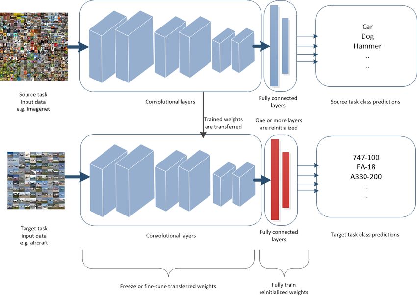
6Fig. 3 Deep transfer learning
images and transferring to medical imaging tasks that if the features stay close to those trained
which often only have 100s of labelled examples. by the large source data set the model will be
So even with the same learning rate and number less likely to overfit.
of epochs, the number of updates to the weights
We describe progress and problems with deep
while training on the target dataset will be orders
transfer learning under these categories as well
of magnitude less than for pretraining. This also
as based on the relationship between source and
prevents the model from creating large weights
target dataset in section 4. Then, in section 5,
that are based on noise or idiosyncrasies in the
we describe how deep transfer learning relates to
small target dataset.
other methods.
Advances in transfer learning can be catego-
rized based on ways of constraining the parame-
ters of W as follows: 3.4 Negative Transfer
1. Initialization. Answering questions like: The stated goal of transfer learning as per Defi-
nition 3 is to improve the learning of the target
• how much pretraining should be done? predictive function fT (.) in DT using the knowl-
• is more source data or more closely related edge in DS and TS . To achieve this goal the
source data better? source dataset must be similar enough to the tar-
• which pretrained parameters should be get dataset to ensure that the features learned
transferred vs reinitialized? in pretraining are relevant to the target task. If
2. Parameter regularization. Regularizing the source dataset is not well related to the tar-
weights, with the assumption that if the get dataset the target model can be negatively
parameters are constrained to be close to a set impacted by pretraining. This is negative transfer
point, they will be less likely to overfit. [91, 108]. Wang et al. [138, 140] define the negative
3. Feature regularization. Regularizing the fea- transfer gap (NTG) as follows:
tures for each training example that are pro-
duced by the weights. Based on the assumption
7Definition 5 ”Let τ represent the test error on the to these inappropriate features. Scenarios such as
target domain, θ a specific transfer learning algorithm this usually lead to overfitting the idiosyncrasies of
under which the negative transfer gap is defined and the target training set [51, 95]. A related scenario
∅ is used to represent the case where the source is explored in [51] where it is shown that alter-
domain data/information are not used by the tar- native loss functions that improve how well the
get domain learner. Then, negative transfer happens
pretrained features fit the source dataset lead to
when the error using the source data is larger than
the error without using the source data: τ (θ(S, τ )) >
a reduction in performance on the target dataset.
τ (θ(∅, τ )), and the degree of negative transfer can be The authors state that ”.. there exists a trade-off
evaluated by the negative transfer gap” between learning invariant features for the original
task and features relevant for transfer tasks.”
N T G = τ (θ(S, τ )) − τ (θ(∅, τ ))
In image classification models, features learned
through lower layers are more general, and those
From this definition we see that negative trans- learned in higher layers are more task specific
fer occurs when the negative transfer gap is pos- [149]. It is likely that if less layers are transferred
itive. Wang et al. elaborate on factors that affect negative transfer should be less prevalent, with
negative transfer [138, 140]: training all layers from random initialization being
the extreme end of this. There has been limited
• Divergence between the source and target
work to test this, however it is shown to an extent
domains. Transfer learning makes the assump-
in [1].
tion that there is some similarity between joint
distributions in source domain PS (X, Y ) and
target domain PT (X, Y ). The higher the diver- 4 Datasets commonly used in
gence between these values the less information transfer learning for image
there is in the source domain that can be
exploited to to improve performance in the tar-
classification
get domain. In the extreme case if there is no 4.1 Source
similarity it is not possible for transfer learning
to improve performance. ImageNet 1K, 5K, 9K, 21K
• Negative transfer is relative to the size and ImageNet is an image database organized accord-
quality of the source and target datasets. For ing to the WordNet hierarchy [18]. ImageNet 1K or
example, if labelled target data is abundant ILSVRC2012 is a well known subset of ImageNet
enough, a model trained on this data only may that is used for an annual challenge. ImageNet
perform well. In this example, transfer learning 1K consists of 1,000 common image classes with
methods are more likely to impair the target at least 1,000 total images in each class for a
learning performance. Conversely, if there is no total of just over 1.3 million images in the train-
labelled target data, a bad transfer learning ing set. ImageNet 5K, 9K and 21K are larger
method would perform better than a random subsets of the full ImageNet dataset containing
guess, which means negative transfer would not the most common 5,000, 9,000 and 21,000 image
happen. classes respectively. All three ImageNet datasets
With deep neural networks, once the weights have have been used as both source and target datasets,
been pretrained to respond to particular features depending on the type of experiments being per-
in a large source dataset the weights will not formed. They are most commonly used as a source
change far from their pretrained values during dataset because of their large sizes and general
fine-tuning [85]. This is particularly so if the target classes.
dataset is orders of magnitude smaller as is often
the case. This premise allows transfer learning to JFT dataset
improve performance and also allows for negative JFT is an internal Google dataset for large-scale
transfer. If the weights transferred are pretrained image classification, which comprises over 300
to respond to unsuitable features then this train- million high-resolution images [40]. Images are
ing will not be fully reversed during the fine-tuning annotated with labels from a set of 18291 cate-
phase and the model could be more likely to overfit gories. For example, 1165 type of animals and 5720
8types of vehicles are labelled in the dataset [125]. Examples of general image classification
There are 375M labels and on average each image datasets commonly used as target datasets are:
has 1.26 labels. • CIFAR-10 and CIFAR-100 [57]: Each have a
total of 50,000 training and 10,000 test images
Instagram hashtag datasets
of 32x32 colour images from 10 and 100 classes
Mahajan et al. [70] collected a weakly labelled respectively.
image dataset with a maximum size of 3.5 billion • PASCAL VOC 2007 [20]: Has 20 classes belong-
labelled images from Instagram, being over 3,000 ing to the superordinate categories of person,
times larger than the commonly used large source animal, vehicle, and indoor objects. It contains
dataset ImageNet 1K. The hashtags were used 9,963 images with 24,640 annotated objects and
as labels for training and evaluation. By varying a 50/50 train test split. The size of each image
the selected hashtags and the number of images is roughly 501 × 375.
to sample, a variety of datasets of different sizes • Caltech-101 [21]: has pictures of objects belong-
and visual distributions were created. One of the ing to 101 categories. About 40 to 800 images
datasets created contained 1,500 hashtags that per category, with most categories having
closely matched the 1,000 ImagNet 1K classes. around 50 images. The size of each image is
roughly 300 × 200 pixels.
Places365 • Caltech-256 [31]. An extension of Caltech-101
Places365 (Places) [155] contains 365 categories of with 256 categories and a minimum of 80 images
scenes collected by counting all the entries that per category. It includes a large clutter category
corresponded to names of scenes, places and envi- for testing background rejection.
ronments in WordNet English dictionary. They
included any concrete noun which could reason- Fine-grained
ably complete the phrase I am in a place, or let’s Fine-grained image classification datasets contain
go to the place. There are two datasets: subordinate classes from one particular superordi-
• Places365-standard has 1.8 million training nate class. examples are:
examples total with a minimum of 3,068 images • Food-101 (Food) [8]: Contains 101 different
per class. classes of food objects with 75,750 training
• Places365-challenge has 8 million training examples and 25,250 test examples.
examples. • Birdsnap (Birds) [7]: Contains 500 different
Places365 is generally used as a source dataset species of birds, with 47,386 training examples
when the target dataset is scene based such as and 2,443 test examples.
SUN. • Stanford Cars (Cars) [55]: Contains 196 dif-
ferent makes and models of cars with 8,144
Inaturalist training examples and 8,041 test examples.
• FGVC Aircraft (Aircraft) [71]: Contains 100 dif-
Inaturalist [131] consists of 859,000 images from
ferent makes and models of aircraft with 6,667
over 5,000 different species of plants and animals.
training examples and 3,333 test examples.
Inaturalist is generally used as a source dataset
• Oxford-IIIT Pets (Pets)[92]: Contains 37 differ-
when the target dataset is when the target dataset
ent breeds of cats and dogs with 3,680 training
contains fine-grained plants or animal classes.
examples and 3,369 test examples.
• Oxford 102 Flowers (Flowers) [89]: Contains 102
4.2 Target different types of flowers with 2,040 training
General examples and 6,149 test examples.
• Caltech-uscd Birds 200 (CUB) [134]: Contains
General image classification datasets contain a
variety of classes with a mixture of superordinate 200 different species of birds with around 60
and subordinate classes from many different cat- training examples per class.
• Stanford Dogs (Dogs) [49]: Contains 20,580
egories in WordNet [77]. ImageNet is a canonical
example of a general image classification dataset. images of 120 breeds of dogs
9Scenes 5 Deep transfer learning
Scene datasets contain examples of different progress and areas for
indoor and/or outdoor scene settings. Examples
are:
improvement
• SUN397 (SUN) [145]: Contains 397 categories In the past decade, the successes of CNNs on
of scenes. This dataset preceded Places-365 and image classification tasks have inspired many
used the same techniques for data collection. researchers to apply them to an increasingly wide
The scenes with at least 100 training examples range of domains. Model performance is strongly
were included in the final dataset. affected by the relationship between the amount of
• MIT 67 Indoor Scenes [98]: Contains 67 Indoor training data and the number of trainable param-
categories, and a total of 15620 images. There eters in a model as shown in Figures 1 and 2. As a
are at least 100 images per category. result there has been ever growing interest in using
transfer learning to allow large CNN models to
Others be trained in domains where there is only limited
training data available or other constraints exist.
There are a number of other datasets that have
As deep learning gained popularity in 2012
less of an overarching theme and are less related
to 2016 transferability of features and best prac-
to the common source datasets. These are often
tices for performing deep transfer learning was
used in conjunction with deep transfer learning
explored [2, 4, 42, 116, 149]. While there are some
for image classification to show models and tech-
recent works that have introduced improvement to
niques are widely applicable. Examples of these
transfer learning techniques and insights, there are
are:
many more that have focused on best practice for
• Describable Textures (DTD) [14]: Consists of either general [52, 61, 70, 96] or specific [37, 100]
3,760 training examples of texture images with application domains rather than techniques. We
47 classes of texture adjectives. fully review both.
• Daimler pedestrian classification [81]: Con- When reviewing the application of deep trans-
tains 23,520 training images with two classes, fer learning for image classification we divide
being contains pedestrians and does not contain applications into categories. We split tasks in two
pedestrians. directions being small versus large target datasets
• German road signs (GTSRB) [123]: Contains and closely versus loosely related source and tar-
39,209 training images of German road signs in get datasets. For example using ImagNet [18] as
43 classes. a source dataset to pretrain a model for classify-
• Omniglot [59]: Contains over 1.2 million train- ing tumours on medical images is a loosely related
ing examples of 1,623 different handwritten transfer and is likely to be a small target dataset
characters from 50 writing systems. due to privacy and scarcity of disease. This cat-
• SVHN digits in the wild (SVHN) [84]: Con- egory division aligns with the factors that affect
tains 73,257 training examples of labelled digits negative transfer outlined in [138, 140].
cropped from Street View images. The distinction between target dataset sizes
• UCF101 Dynamic Images (UCF101) [121]: Con- is useful as it has been shown that small target
tains 9,537 static frames of 101 classes of actions datasets are much more sensitive to changes in
cropped from action videos. transfer learning hyperparameters [95]. It has also
• Visual Decathlon Challenge (Decathlon) [103]: been shown that standard transfer learning hyper-
A challenge designed to simultaneously solve paramters do not perform as well when trans-
10 image classification problems being: Ima- ferring to a less related target task [34, 52, 96],
geNet, CIFAR-100, Aircraft, Daimler pedes- with negative transfer being an extreme example
trian, Describable textures, German traf- of this [138, 140], and that the similarity between
fic signs, Omniglot, SVHN, UCF101, VGG- datasets should be considered when deciding on
Flowers. All images resized to have a shorter hyperparameters [61, 96]. These distinctions go
side of 72 pixels some way to explaining conflicting performance
10of deep transfer learning methods in recent years related, particularly with smaller target datasets
[34, 61, 135, 159]. [1, 95, 96].
We start this section by describing general More recently it has been shown that the per-
studies on deep transfer learning techniques, formance of models on ImageNet 1K correlates
including recent advances. Then we review work well with performance when the pretrained model
in each of the application areas described by our is transferred to other tasks [52]. The authors
split above. Section 7 summarizes current knowl- additionally demonstrate that the increase in per-
edge and makes final recommendation for future formance of deep transfer learning over random
directions of research in the field. initialization is highly dependent on both the tar-
get dataset size and the relationship between the
5.1 General deep transfer learning classes in the source and target datasets. This will
for image classification be discussed more in the following sections.
Early work on deep transfer learning showed that: 5.2 Recent advances
1. Deep transfer learning results in comparable Recent advances in the body of knowledge related
or above state of the art performance in many to deep transfer learning for image classification
different tasks, particularly when compared to can be divided into advances in techniques, and
shallow machine learning methods [4, 116]. general insights on best practice. We describe
2. More pretraining both in terms of the number advances in transfer learning techniques here and
of training examples and the number of iter- insights on best practice in Section 5.2.4. Recent
ations tends to result in better performance advances in techniques are divided into regulariza-
[2, 4, 42]. tion, hyperparameter based, matching the source
3. Fine-tuning the weights on the target task domain to the target domain, and a few others
tends to result in better performance particu- that do not fit the previous categories. We discuss
larly when the target dataset is larger and less matching the source domain to the target domain
similar to the source dataset [2, 4, 149]. under the relevant source versus task domains in
4. Transferring more layers tends to result in bet- Sections 5.3.1 and 5.6.1 and the rest below. In
ter performance when the source and target our reviews of recent work we attempt to present
dataset and task are closely matched, but less a balanced view of the evidence for the improve-
layers are better when they are less related ments offered by newer models compared to prior
[1, 2, 4, 13, 149]. ones and the limitations of those improvements.
5. Deeper networks result in better performance However, in some of the more recent cases this is
[4]. difficult as the original papers provide limited evi-
It should be noted that all the studies referenced dence and new work showing the limitations of the
above were completed prior to advances in resid- methods has not yet been done.
ual networks [36] and other modern very deep
CNNs. It has been argued that residual networks 5.2.1 Regularization based technique
when combined with fine-tuning makes features advances
more transferable [36]. As many of the above
Most regularization based techniques aim to solve
studies were carried out within a similar time
the problem of the unreliable empirical risk mini-
period some results have not been combined. For
mizer 3.2.2 by restricting the model weights or the
instance, most were done with AlexNet, a rela-
features produced by them so they can’t fit small
tively shallow network, as a base and many did
idiosyncrasies in the data. They achieve this by
not perform fine tuning and/or simply used a deep
adding a regularization term λ · Ω (.) to the loss
neural network as a feature detector at whatever
function to make it:
layer it was transferred. It has since been shown
that when fine-tuning is used effectively, transfer-
ring less than the maximum number of layers can ( n
)
1X
result in better performance. This applies even minw L (w) = L (z (xi , w) , yi ) + λ · Ω (.)
when the source and target datasets are highly n i=1
11Pn
with the first term n1 i=1 L (z (xi , w) , yi ) two source datasets used for pretraining. It
being the empirical loss and the second term being has since been shown that the L2-SP regular-
the regularization term. The tuning parameter izer can result in minimal improvement or even
λ > 0 balances the trade-off between the two. negative transfer when the source and target
Weight regularization directly restricts how datasets are less related [12, 61, 96, 135]. More
much the model weights can move. recent work has showed that in some cases
Knowledge distillation or feature based regu- using L2-SP regularization for lower layers and
larization uses the distance between the feature L2 regularization for higher layers can improve
maps output from one or more layers of the source performance [96].
and target networks to regularize the model: 2. DELTA [63] is an example of knowledge distil-
lation or feature map based regularization. It
is based on the idea of re-using CNN channels
N n
1 XX that are not useful to the target task while not
Ω(w, ws ) = d (Fj (wt , xi ) , Fj (ws , xi ))
n j=1 i=1 changing channels that are useful. Training on
the target task is regularized by the attention
where Fj (wt , xi ) is the feature map output weighted L2 loss between the final layer feature
by the jth filter in the target network defined by maps of the source and target models:
weights wt for input value xi , and d (.) is a measure N
of dissimilarity between two feature maps.
X
Ω(w, w0 , xi , yi ) = (Wj (w0 , xi , yi )
The success of regularization based techniques j=1
for deep transfer learning rely heavily on the 2
assumption that the source and target datasets · F Mj (w, xi ) − F Mj (w0 , xi )) 2
are closely related. This is required to ensure
that the optimal weights or features for the tar- Where F Mj (w, xi ) is the output from the jth
get dataset are not far from those trained on the filter applied to the ith input. The attention
source dataset. weights Wj for each filter are calculated by
There have been many new regularization removing the model’s filters one by one (set-
based techniques introduced in the last three ting its output weights to 0), calculating the
years. We review major new techniques in chrono- increase in loss. Filters resulting in a high
logical order. increase in loss are then set with a higher
weight for regularization, encouraging them to
1. L2-SP [64, 65] is a form of weight regulariza- stay similar to those trained on the source task.
tion. The aim of transfer learning is to create Others that are not as useful in the target task
models that are regularized by keeping features are less regularized and can change more. This
that are reasonably close to those trained on regularization resulted in performance that was
a source dataset for which overfitting is not slightly better than the L2-SP regularization in
as much of a problem. The authors argue that most cases with ResNet-101 and Inceptionv3
because of this, during the target dataset train- models, ImageNet 1K as the source dataset
ing phase the fine tuned weights should be and a variety of target datasets. The original
decayed towards the pretrained weights, not paper showed state of the art performance for
zero. Several regularizers that decay weights DELTA on Caltech 256-30, however they used
towards their starting point, denoted SP reg- mostly the same datasets as the original L2-SP
ularizers, were tested in the original papers. paper [64] and for the two additional datasets
2
The L2-SP regularizer Ω(w) = α2 w − w0 2 used they showed that L2-SP outperformed the
which is the L2 loss between the source weights baseline L2 regularization. It has since been
and the current weights is shown to signif- shown that like L2-SP, DELTA can also hin-
icantly outperform the standard L2 loss on der performance when the source and target
the four target datasets shown in the paper datasets are less similar [12, 45, 53].
with a Resent-101 model. The original paper 3. Wan et al. [135] propose decomposing the
showed results for transferring to four small transfer learning gradient update into the
target datasets that were very similar to the empirical loss and regularization loss gradient
12vectors. Then when the angle between the two 5.2.2 Normalization based technique
vectors is greater than 90 degrees they fur- advances
ther decompose the regularization loss gradient
Further to regularization based methods, there
vector into the portion perpendicular to the
are several recent techniques that attempt to bet-
empirical loss gradient and the remaining vec-
ter align fine-tuning in the target domain with
tor in the opposite direction of the empirical
the source domain. This is achieved by making
loss gradient. They remove the latter term,
adjustments to the standard batch normalization
in the hopes that not allowing the regulariza-
or other forms of normalization that are used
tion term to move the weights in the opposite
between layers in modern CNNs.
direction of the empirical loss term will stop
negative transfer. They show that their pro- 1. Sharing batch normalization hyperparameters
posal improves performance slightly with a across source and target domains has been
ResNet 18 on four different datasets. However, shown to be more effective than having sep-
their results are poor compared to state of the arate ones across many domain adaptation
art as they do not test on modern very deep tasks [72, 138]. Wang et al. [138] introduce
models. For this reason, it is difficult to judge an additional batch normalization hyperpa-
how well their regularization method performs rameter called domain adaptive α. This takes
in general. standard batch normalization with γ and β
4. Batch spectral shrinkage (BSS) [12] introduces shared across source and target domain and
a loss penalty applied to smaller singular values scales them based on the transferability value
of channelwise features in each batch update of each channel calculated using the mean and
during fine-tuning so that untransferable spec- variance statistics prior to normalization. As
tral components are suppressed. They test this far as we are aware these techniques have not
method using a ResNet50 pretrained on Ima- been applied to the general supervised transfer
geNet 1K and fine-tuned on a range of different learning case.
target datasets. The results show that their 2. Stochastic normalization [53] samples batch
method never hurts performance on the given normalization based on mini-batch statistics
datasets and often produces significant per- or based on moving statistics for each fil-
formance gains over L2, L2-SP and DELTA ter with probability hyperparameter p. At the
regularization for smaller target datasets. They start of fine-tuning on the target dataset the
also show that BSS can improve performance moving statistics are initialised with those cal-
for less similar target datasets where L2-SP culated during pretraining in order to act as a
hinders performance. regularizer. This is designed to overcome prob-
5. Sample-based regularization [45] proposes reg- lems with small batch sizes resulting in noisy
ularization using the distance between feature batch-statistics or the collapse in training asso-
maps of pairs of inputs in the same class, ciated with using moving statistics to normalize
as well as weight regularization. The model all feature maps [43, 44]. The authors results
was tested using a ResNet-50 and transfer- show that their methods improve over BSS,
ring from ImageNet 1K and Places365 to a DELTA and L2-SP for low sampling versions
number of different, fine grained classification of three standard target datasets and improve
tasks. The authors report an improvement over over all but BSS for larger versions of the
L2-SP, DELTA and BSS in all tests. Their same datasets. Their results again show that
results reconfirm that BSS performs better BSS performs better than DELTA and L2SP
than DELTA and L2SP in most cases and in in most cases and in many cases DELTA and
some cases DELTA and L2SP decrease perfor- L2-SP decrease performance compared to the
mance compared to the standard L2 regular- standard L2 regularization baseline.
ization baseline.
5.2.3 Other recent new techniques
Guo et al. [32] make two copies of their ResNet
models pretrained on ImageNet 1K. One model is
13used as a fixed feature selector with the pretrained Given a set of models with similar accuracy on
layers frozen and the other model is fine-tuned. a source task, the best model for target tasks
They reinitialize the final classification layer in can vary between target datasets [1].
both. A policy net trained with reinforcement • Choosing the best data for pretraining. In many
learning is then used to create a mask to com- cases pretraining with smaller more closely
bine layers from each model together in a unique related source datasets was found to produce
way for each target example. They show that better results on target datasets than with
their SpotTune model improves performance com- larger less closely related source datasets [16,
pared to fine-tuning with an equivalent size single 17, 70, 76, 87, 97]. For best results the source
model (double the size of the two individual mod- dataset should include the image domain of the
els within the SpotTune architecture) and achieves target dataset [76]. For example ImageNet 1k
close to or better than state of the art in most contains more classes of pets than Oxford Pets
cases. MultiTune simplifies SpotTune by removing making them an ideal source and target dataset
the policy network and concatenating the features combination. There are various measures of sim-
from each model prior to the final classification ilarity used to define closely related that are
layer rather than selecting layers. It also improves outlined in Section 5.3.1.
on SpotTune by using two different non-binary • Finding the best hyperparameters for fine-
fine-tuning hyperparameter settings [96] rather tuning. Several studies include extensive hyper-
than one fine-tuned and one frozen model. The parameter searches over learning rate, learning
results show that MultiTune improves or equals rate decay, weight decay, and momentum [52,
accuracy compared to SpotTune in most cases 61, 64, 70, 96]. These studies show the rela-
tested, with significantly less training time. tionship between the size of the target dataset
Co-tuning for transfer learning [150] uses a and its similarity to the source dataset with
probabilistic mapping of hard labels in the source fine-tuning hyperparameter settings. Optimal
dataset to soft labels in the target dataset. This learning rate and momentum, are both shown
mapping allows them to keep the final classifica- to be lower for more related source and tar-
tion layer in a ResNet50 and train it using both get datasets [61, 96]. Also the number of layers
the target data and soft labels from the source to reinitialise from random weights is strongly
dataset. As with many other recent results, they related to the optimal learning rate [85, 96].
show that their algorithm improves on all others, • Whether a multi-step transfer process is better
including BSS, DELTA and L2SP, but their results than a single step process. A multi-step pretrain-
are significantly below state of the art for identi- ing process, where the intermediate dataset is
cal model sizes, source and target dataset. They smaller and more closely related to the target
do show the same ordering for the target datasets, dataset, often outperform a single step pre-
using BSS improves on DELTA which improves on training process when originating from a very
L2SP. different, large source dataset [28, 76, 86, 97].
Related to this, using a self-supervised learn-
5.2.4 Insights on best practice ing technique for pretraining on a more closely
related source dataset can outperform using a
Further to advances in techniques and models,
supervised learning technique on a less closely
there has been a large body of recent research that
related dataset [159].
extends the early work on best practice for deep
• Which type of regularization to use. L2-SP
transfer learning for image classification described
or other more recent transfer learning specific
in Section 5.1. These studies give insights on
regularization techniques like DELTA, BSS,
the following decisions that need to be made
stochastic normalization, etc, improve perfor-
when performing deep transfer learning for image
mance when the source and target dataset are
classification:
closely related, but often hinder it when they
• Selecting the best model for the task. Models are less related [63, 64, 96, 135]. These regular-
that perform better on ImageNet were found to ization techniques are discussed in more detail
perform better on a range of target datasets in in Section 5.2.1.
[52], however this effect eventually saturates [1].
14• Which loss function to use. Alternatives to making them easier to transfer to. Their final tar-
the cross-entropy loss function are shown to get dataset, Flowers, is also known to be better
produce representations with higher class sepa- suited to transfer to from their source datasets.
ration that obtain higher accuracy on the source See section 5.6 for further discussion of which
task, but are less useful for target tasks in [51]. target datasets are easier to transfer to.
The results show a trade-off between learning We expect that best practice recommendations
features that perform better on the source task developed for closely related datasets will not be
and features relevant for the target task. applicable to less closely related target datasets as
has been shown for many other methods and rec-
In an attempt to generalize hyperparame-
ommendations [12, 53, 61, 63, 64, 96, 135]. To test
ters and protocols when pretraining with source
this hypothesis we reran a selection of the exper-
source datasets that are larger than ImageNet 1K,
iments in BiT using Stanford Cars as the target
Kolesnikov et al. created Big Transfer (BiT) [50].
dataset which is very different from the source
They pretrain various sizes of ResNet on Ima-
dataset ImageNet 21K and known to be more diffi-
geNet 1K and 21K, and JFT and transfer them
cult to transfer to [52, 96]. We first confirmed that
to four small to medium closely related image
we could reproduce their state of the art results
classification target datasets as well as the COCO-
for the datasets listed in the paper, then produced
2017 object detection dataset [66]. Based on these
the results in Table 1 using Stanford Cars. These
experiments they make a number of general claims
results show that BiT produces far below state of
about deep transfer learning when pretraining on
the art results for this less related dataset. The
very large datasets including:
first column shows the results with all the recom-
1. Batch normalization (BN) [44] is detrimental mended hyperparameters from the paper. While
to BiT, and Group Normalization [144] com- the performance can be improved with increases
bined with Weight Standardization performs in learning rates and number of epochs before the
well with large batches. learning rate is decayed, final results are still well
2. MixUp [151] is not useful for pretraining on below state of the art for a comparable model,
large source datasets and is only useful dur- source and target dataset. The fine grained clas-
ing fine-tuning for mid-sized target datasets sification task in Stanford Cars is known to be
(20-500K training examples) less similar to the more general ImageNet and
3. Regularization (L2, L2-SP, dropout) does not JFT datasets. Because of this it is not surprising
enhance performance in the fine-tuning phase, that recommendations developed for more closely
even with very large models (the largest model related target datasets do not apply.
used for experiments has 928 million parame-
ters). Adjusting the training and learning rate 5.2.5 Insights on transferability
decay time based on the size of the target
Here we review works that give more general
dataset, longer for larger datasets, provides
insight as to what is happening with model
sufficient regularization.
weights, representations and the loss landscape
The authors use general fine-tuning hyperparame- when transfer learning is performed as well as
ters for learning rate scheduling, training time and measures of transferability of pretrained weights
amount/usage of MixUp that are only adjusted to target tasks.
based on the target dataset size, not for individual Several methods for analysing the feature
target datasets. They achieve performance that space were used in [85]. They found that mod-
is comparable to models with selectively tuned els trained from pretrained weights make similar
hyperparameters for their model pretrained on mistakes on the target domain, have similar fea-
ImageNet and state of the art, or close to in many tures and are surprisingly close in `2 distance in
cases, for their model pretrained on the 300 times the parameter space. They are in the same basins
larger source dataset JFT. However their target of the loss landscape. Models trained from random
datasets, ImageNet, CIFAR 10 & 100, and Pets initialization do not live in the same basin, make
are very closely related to their source datasets different mistakes, have different features and are
farther away in `2 distance in the parameter space.
15Table 1 Big transfer (BiT): General visual representation learning [50] extended results using BiT-M pretrained on
ImageNet 21K . State of the art is the best known result for this model, source and target dataset. Default is the learning
rate decay schedule specified by the paper for this size target dataset and x2 is two times the number of batches before
decaying the learning rate compared to the default.
Dataset Default lr (0.003) lr 0.01 lr 0.03 lr 0.1 State of the art
default x2 default x2 default x2 default x2
decay decay decay decay
Cars 86.20 86.15 85.81 87.49 81.41 88.96 27.51 5.22 95.3[87]
A flatter and easier to navigate loss landscape They then define conditional cross-entropy
for pretrained models compared to their randomly (NCE) as another measure of transferability,
initialized counterparts was also shown in [67]. defined as being the empirical cross entropy
They showed improved Lipschitzness and that this of label ȳ from the target domain given a
accelerates and stabilizes training substantially. lablel z̄ from the source domain. To empiri-
Particularly that the singular vectors of the weight cally demonstrate the effectiveness of the NCE
gradient with large singular values are shrunk in measure a ResNet18 model as the backbone
the weight matrices. Thus, the magnitude of gradi- was paired with an SVM classifier. NCE was
ent back-propagated through a pretrained layer is demonstrated to have strong correlation with
controlled, and pretrained weight matrices stabi- accuracy on the target tasks for combinations
lize the magnitude of gradient, especially in lower of 437 source and target tasks.
layers, leading to more stable training. 3. LEEP [88] is another measure of transferability.
Several recent techniques have been proposed Using the pretrained model, the joint distri-
for measuring the transferability of pretrained bution over labels in the source dataset and
weights: the target dataset labels is estimated to con-
struct an empirical predictor. LEEP is the log
1. H-score [5] is a measure of how well a pretrained
expectation of the empirical predictor. LEEP
model f is likely to perform on a new task with
is defined mathematically as:
input space X and output space Y based on
the inter-class covariance cov(EPX|Y [f (X)|Y ]) n
!
and the feature redundancy tr(cov(f (X))) 1X X
T (θ, D) = log P̂ (yi |z) θ (xi )z
n i=1
zZ
H(f ) = tr(cov(f (X))−1 cov(EPX|Y [f (X)|Y ])
where θ (xi )z is is the probability of the source
the H-score increases as interclass covariance label z for target input data xi predicted using
increases and feature redundancy decreases. the pretrained weights θ, and P̂ (yi |z) is the
The authors show that H-score has a strong empirical conditional probability of target label
correlation with target task performance. They yi given source label z. LEEP is shown to have
also show that it can be used to rank transfer- good theoretical properties and empirically it
ability and create minimum spanning trees of is demonstrated to have strong correlation with
task transferability. The latter may be useful performance gain from pretraining weights on
in guiding multi-step transfer learning for less the source tasks. This is shown on source tasks
related tasks as discussed in Section 5.2.4. ImageNet 1K and CIFAR10 and 200 random
2. Transferability and negative conditional target tasks taken from the closely related
entropy (NCE) for transfer learning tasks CIFAR100 and less closely related FashionM-
where the source and target datasets are NIST. The authors expand NCE to the case
the same, but the tasks differ, are defined where the source and target datasets are dif-
in [130]. The authors define transferability ferent by creating dummy labels for the target
as the log-likelihood lY (wZ , kY ), where wz is data based on the source task using the pre-
the weights of the model backbone pretrained trained model θ. They show that LEEP has
on the source task Z and kY is the weights a stronger correlation with performance gain
of the classifier trained on the target task. than the expanded NCE measure and H-score.
16You can also read