DEFORESTATION DETECTION IN THE AMAZON RAINFOREST WITH SPATIAL AND CHANNEL ATTENTION MECHANISMS - The International Archives of ...
←
→
Page content transcription
If your browser does not render page correctly, please read the page content below
The International Archives of the Photogrammetry, Remote Sensing and Spatial Information Sciences, Volume XLIII-B3-2021
                                                  XXIV ISPRS Congress (2021 edition)

             DEFORESTATION DETECTION IN THE AMAZON RAINFOREST WITH
                   SPATIAL AND CHANNEL ATTENTION MECHANISMS

                                              P. Tovar1, ∗, M. O. Adarme1 , R. Q. Feitosa1
                           1
                      Department of Electrical Engineering, Pontifical Catholic University of Rio de Janeiro,
           22451-900 Rio de Janeiro, Brazil - (ptovar@opto.cetuc.puc-rio.br, mortega@ele.puc-rio.br, raul@ele.puc-rio.br)

KEY WORDS: Remote Sensing, Deforestation Detection, Attention Mechanisms, Convolutional Neural Networks.

ABSTRACT:

Deforestation in the Amazon rainforest is an alarming problem of global interest. Environmental impacts of this process are
countless, but probably the most significant concerns regard the increase in CO2 emissions and global temperature rise. Currently,
the assessment of deforested areas in the Amazon region is a manual task, where people analyse multiple satellite images to quantify
the deforestation. We propose a method for automatic deforestation detection based on Deep Learning Neural Networks with dual-
attention mechanisms. We employed a siamese architecture to detect deforestation changes between optical images in 2018 and
2019. Experiments were performed to evaluate the relevance and sensitivity of hyperparameter tuning of the loss function and the
effects of dual-attention mechanisms (spatial and channel) in predicting deforestation. Experimental results suggest that a proper
tuning of the loss function might bring benefits in terms of generalisation. We also show that the spatial attention mechanism is
more relevant for deforestation detection than the channel attention mechanism. When both mechanisms are combined, the greatest
improvements are found, and we reported an increase of 1.06% in the mean average precision over a baseline.

                      1. INTRODUCTION                                 regular activities and contribute to climate change mitigation.
                                                                      In this regard, Remote Sensing (RS) has demonstrated to be a
The environmental impacts of deforestation in the Amazon              cost-effective solution to monitor these regions. The advances
rainforest have been attracting research interest for many dec-       of this technology and the easy access to high-resolution images
ades (Lean, Warrilow, 1989, Shukla et al., 1990). As this region      throughout the globe propelled remote sensing Change Detec-
is the largest tropical forest globally, it is paramount to assess    tion (CD) techniques.
its deforestation consequences. Countless works report predic-
tions on climate changes due to deforestation in the Amazon           Many approaches have been proposed to enhance CD perform-
rainforest. For instance, Swann and co-workers developed a re-        ance. Mostly, we can group them into four main categories: im-
gional ecosystem model to investigate the future consequences         age algebra; transformation; time-series analysis and classifica-
of climate changes caused by deforestation in South Amer-             tion (Hecheltjen et al., 2014). Image algebra methods are based
ica (Swann et al., 2015). Medvigy simulated the effects of            on spectral values analysis, and they range from simple image
Amazon deforestation in the northern hemisphere climate using         differencing to change vector analysis (CVA), which calculates
the Ocean-Land-Atmosphere Model, where significant temper-            both the magnitude and direction of changes. Methods that con-
ature and precipitation changes were predicted (Medvigy et al.,       vert the input data into another dimensional-space for change
2013). However, the effects of deforestation are not restricted       analysis are part of the transformation category. Examples of
to changes in temperature and precipitation. Deforestation for        transformation methods are Fast Fourier Transform (FFT) and
land use is dual-severe in terms of greenhouse gases because at       Principal Component (PC) based change detection (Wiemker,
the same time that it is one of the largest causes of anthropo-       1997). Time-series analysis encompasses the methods using
genic CO2 emissions; it also ends up reducing the natural capa-       more than two images of the same location taken at different
city of terrestrial carbon storage (Sy et al., 2015). Furthermore,    times to detect the changing trends. The last category cov-
deforestation has an enormous impact on biodiversity loss, be-        ers classification methods, which relies on a great quantity and
ing even more harmful to species of high conservation and func-       quality of classified images to produce change detection out-
tional value (Barlow et al., 2016). Besides these more evident        puts (Lu et al., 2004).
effects, there are also indirect and hard to predict consequences
of deforestation. An example is a recent study that relates the       Classification methods for CD started to stand out due to the
increase of malaria transmission in Brazil due to Amazon de-          remarkable results of Deep Learning (DL) applied to image
forestation (MacDonald, Mordecai, 2019).                              classification. Since then, DL classification methods have been
                                                                      widely used for various CD applications, including land use and
According to National Institute for Space Research, the defor-        land cover change, urban settlements, changes caused by nat-
ested areas in Amazon decreased almost steadily from 2004 to          ural catastrophes, and deforestation changes (Asokan, Anitha,
2014 (INPE, 2020). However, in the last years, the deforest-          2019). Given the importance of deforestation detection in the
ation processes have significantly increased, reaching in 2019        Amazon rainforest, methods based on DL have been applied to
the largest deforested area in the past ten years. Therefore, this    this problem aiming to provide a robust and automatic way to
forest’s supervision is essential to control man-made hazards         monitor Amazon deforested areas (Ortega Adarme et al., 2020,
and natural disasters and enforce public policies to avoid ir-        de Bem et al., 2020).
∗   Corresponding author                                              In this work, a recently proposed deep-learning method for

                                                 This contribution has been peer-reviewed.
                  https://doi.org/10.5194/isprs-archives-XLIII-B3-2021-851-2021 | © Author(s) 2021. CC BY 4.0 License.             851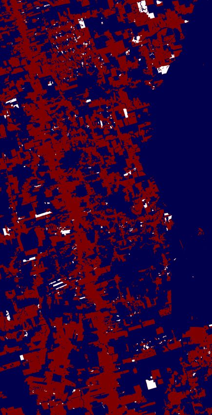
The International Archives of the Photogrammetry, Remote Sensing and Spatial Information Sciences, Volume XLIII-B3-2021
                                                 XXIV ISPRS Congress (2021 edition)

CD (Chen et al., 2020) was applied to deforestation detection        2020, Maretto et al., 2020). However, despite the positive res-
in the Amazon rainforest. The methodology’s main idea is             ults, current methods are still sensitive to pseudo-changes. For
to use dual-attention mechanism (spatial and channel) to im-         instance, some areas might be misclassified as deforested be-
prove the robustness against pseudo-changes in remote sens-          cause they have a different luminosity, shadow, noise, or any
ing applications, i.e., efficiently distinguishing between relev-    other factor that might mislead the neural network. Yet, this
ant changes and circumstantial ones, such as noise and context.      problem is not restricted to deforestation detection but rather
This concept, which will be described in details in the follow-      common to most CD applications. Aiming to mitigate this prob-
ing sections, has great potential for deforestation detection, and   lem for change detection between images taken at different sea-
in this case, the relevant change is current deforestation itself.   sons, Chen proposed the usage of extended self-attention mech-
Furthermore, Chen’s approach (Chen et al., 2020) uses a new          anism (Chen et al., 2020).
loss function, which intends not only to compensate for the im-
balance problem often found in training samples but also to op-      2.2   Attention Mechanisms
timise the training process.                                         When reading a sentence, humans naturally focus their attention
This paper is organised as follows. Section 1 describes the rel-     on the most relevant words. Although each word has its import-
evance of deforestation detection in the Amazon rainforest and       ance grammatically, some words give much more information
how it has been approached with recent DL methods. Section 2         than others. The same happens with images. We pay more
covers the related works in the literature. In section 3 it is de-   attention to regions in images providing more context informa-
tailed the methodology used in this work, where the network          tion. For instance, by looking at an image of a cat playing with a
architecture, attention mechanisms and loss function are ex-         ball at a backyard, we rapidly focus on the cat’s primary features
plained. Section 4 presents the experiments assessed and their       - pointy ears, paws, feline nose and mouth - and on the ball’s
results. Finally, Section 5 concludes the work.                      spherical shape, not paying much attention to the background.
                                                                     This natural capability of focusing on more relevant features is
                                                                     key for image classification, as only the most significant aspects
                   2. RELATED WORKS                                  are learned, making us exceptional in generalization tasks. Re-
                                                                     cently, this attention concept has been brought to deep learning
2.1   Deforestation Detection                                        algorithms.
The number of papers studying deforestation detection using          Attention mechanisms (AM) were first proposed in (Bahdanau
DL techniques increased considerably in the past few years. Re-      et al., 2015) to solve the long-range dependence issue of
cently, a Convolutional Neural Network (CNN) was employed            sequence-to-sequence models. Since then, AM have been ex-
by Grings to monitor deforestation events based on an 18-years       plored in several applications (Xu et al., 2019, Mahayossanunt
time-series of Enhanced Vegetation Index (EVI) in the Chaco          et al., 2019, Li et al., 2020). The principal idea of AM is to
Forest (Grings et al., 2020). The EVI is a vegetation index          allow to the network focus on more meaningful features by
based on the spectral content of satellite images. It oscillates     weighting them according to their importance. Hu et al. re-
according to seasonal changes, but the oscillation exhibits a        ported an interesting configuration of AM by defining Squeeze-
break-point in a deforestation event. Grings’ model was trained      and-Excitation (SE) blocks (Hu et al., 2018), which were de-
to learn the break-points’ patterns, estimating the probability      signed to model the interdependencies between image channels
of deforestation for a given EVI sequence. The model showed          explicitly.
to be sensitive to mislabeled deforestation events, which limited
its performance. Also, it requires long EVI time-series for train-   Other researches extended the concept of Channel Attention
ing, which are often unavailable. And since the CNN is trained       Mechanism to the spatial dimension (Guo et al., 2018). For
with samples of EIV time-series, the spatial relation of pixels      instance, in (Roy et al., 2019), the performance of SE atten-
is not considered in the learning process. A similar work re-        tion blocks was assessed separately for channel and spatial di-
ported by Adarme and co-workers (Ortega Adarme et al., 2020)         mensions and in a joint channel-spatial attention configuration.
evaluated the performance of three DL algorithms applied to          Tests with these three configurations were performed with med-
the deforestation detection problem in two different Brazilian       ical imagery for semantic segmentation, and most results out-
biomes: Amazon and Cerrado. The assessed strategies were             performed configurations without AM.
a CNN, Siamese Network, Convolutional Support Vector Ma-
                                                                     For change detection applications, a similar idea was proposed
chine and Support Vector Machine. The obtained results were
                                                                     by Chen and co-workers. Dual-attention mechanisms, acting
promising. However, all these methods rely on a patch-wise
                                                                     both on the channel and spatial dimensions, were included in
classification, which can be computationally intensive.
                                                                     a siamese network architecture to improve robustness against
An analysis considering a Fully Convolutional Networks (FCN)         pseudo-changes, primarily seasonal. Results showed consistent
was successfully applied and reported in (de Bem et al., 2020).      improvement in all metrics evaluated (Chen et al., 2020). These
The dataset consists of images from the Amazon territory ac-         results suggest that the performance of state-of-the-art deep-
quired one year apart. Training samples were formed by stack-        learning architectures used for deforestation detection could be
ing two images from the same location at different years. It was     improved with dual-attention mechanisms. In our work, we im-
evaluated the performance of five different architectures on the     plemented the concepts of dual-attention mechanisms to defor-
task of deforestation classification: SharpMask, U-Net, Res-         estation detection in the Amazon rainforest.
Net, Random Forest and Multilayer Perceptron. The firsts three
architectures produced better classification results than the last                       3. METHODOLOGY
two, showing that DL approaches are better suited for RS ap-
plications than classic machine-learning algorithms.                 3.1   Network Architecture

Other works with similar approaches also reported remarkable         The network architecture is shown in Figure 1. Its input is com-
results using DL methods for deforestation detection (Lee et al.,    posed of two co-registered images of the same area acquired

                                                This contribution has been peer-reviewed.
                 https://doi.org/10.5194/isprs-archives-XLIII-B3-2021-851-2021 | © Author(s) 2021. CC BY 4.0 License.              852
The International Archives of the Photogrammetry, Remote Sensing and Spatial Information Sciences, Volume XLIII-B3-2021
XXIV ISPRS Congress (2021 edition)
at different times, shown as IT0 and IT1 . Both images un- v SAM , respectively. These are defined as follows,
dergo the same transformations throughout the network, i.e.,
N et 0 and N et 1 share all weights, denoting a siamese relation. q SAM = reshape(CON V1 (fX 1 ))T
Each input image is transferred to an embedding space through k SAM = reshape(CON V1 (fX 1 )) (1)
a sequence of convolutions, non-linear activations (ReLU) and
v SAM = reshape(CON V2 (fX 1 )),
max-pooling operations (convs in Figure 1), leading to features
f 0 1 and f 1 1 . Then, each feature is sent through an attention
block, where two attention mechanisms take place. Details of where fX 1 ∈ RCIN ×H×W is the input of the attention block,
the attention block operations will be described in section 3.2. such that X can assume values {0, 1}, depending on the net-
Still, it can be understood as a transformation block that gener- work analysed (N et0 or N et1 ). The operations CON V1 and
ates a feature embedding of the same size of its input but with CON V2 are 1 × 1 convolutions with output channels N and
channel and spatial features weighted by their own importance. CIN , respectively. Applying CON V1 to fX 1 gives a tensor in
the space RN ×H×W . k SAM is obtained by reshaping the out-
put of this convolution to the tensorial space RN ×H∗W . The
The outputs of the attention blocks, f 0 2 and f 1 2 , are used in query, q SAM , is calculated by transposing a reshaped con-
a distance function d(·, ·) to compute the pixel-wise distance volved tensor, giving an element in RH∗W ×N . The value,
between feature embeddings. Last, a bi-linear upsample op- v SAM , is obtained by reshaping the output of a 1 × 1 con-
eration is applied to the distance function output, generating volution with CIN channels, resulting in a tensor in space
a change map of the same size of the input images. The up- RCIN ×H∗W .
sampled change map and deforestation label are used to calcu-
late the loss, which is a contrastive function with two margins,
as will be explained in section 3.3.
The central element of the SAM is the calculus of the spatial
attention tensor A SAM , which is given by
A SAM = σ(q SAM · k SAM ), (2)
where σ is the softmax operation. Note that A denotes a mul-
tiplication between matrices of dimensions (H ∗ W, N ) and
(N, H ∗ W ), such that the output resides in space RH∗W ×H∗W .
We can think of this operation as a contraction in the channel
dimension, resulting in a tensor that provides spatial-context re-
lations. The softmax operation guarantees that the values of A
lies in the interval [0, 1]. Next, we apply the attention tensor
to the value v SAM and reshape the output to have the same di-
mension of the input fX 1 , i.e.
s SAM = reshape(v SAM · A SAM ), (3)
Figure 1. Network architecture.
with s SAM ∈ RCIN ×H×W . Last, we write the output of the
SAM as a sum between the input fX 1 and s SAM weighted
3.2 Attention Mechanisms by a learnable parameter η , such that the neural network will
learn the relevance of the SAM. Thus, the output of SAM can
be written as:
The type of attention mechanism implemented in this work is
defined as self-attention. Its goal is to generate a better repres-
out SAM = fX 1 + η s SAM (4)
entation of a given feature embedding by focusing on more rel-
evant elements of the embedding itself, i.e., without additional For the CAM we have similar key, query and value tensors, but
information. Since feature embeddings of images are usually no convolutions are used (Chen et al., 2020). These are defined
represented as tensors with at least three dimensions, it is pos- as follows:
sible to force an attention mechanism to focus on a specific q CAM = reshape(fX 1 )
dimension. In this section, we detail the two attention mech-
anisms that rely within the attention block shown in Figure 1, k CAM = reshape(fX 1 )T (5)
one focusing on the spatial dimension and the other on the chan- v CAM = reshape(fX 1 ).
nel dimension. Henceforth, these will be referred to as Spatial
Attention Mechanism (SAM) and Channel Attention Mechan- The paramount difference between Equations 1 and 5 is the
ism (CAM). position of the transpose operation. It the former, it is ap-
plied to the query, while in the latter it is applied to the key.
Thus, q CAM resides in the space RCIN ×H∗W and k CAM in
Both SAM and CAM uses the concept of query, key and value RH∗W ×CIN . With this modification, when multiplying these
to implement self-attention, which has been used in a similar elements as done in Equation 2 for the SAM case, we obtain a
way in (Ramachandran et al., 2019). This concept is borrowed channel attention tensor with dimension (CIN , CIN ), given by
from retrieval systems, where it is realised a similarity measure-
ment between a query and keys to return a match with the best A CAM = σ(q CAM · k CAM ). (6)
value. We start by analysing the operations for the SAM. Let us
represent query, key and value for SAM as q SAM , k SAM and In a similar way as done before for the SAM case, we calculate
This contribution has been peer-reviewed.
https://doi.org/10.5194/isprs-archives-XLIII-B3-2021-851-2021 | © Author(s) 2021. CC BY 4.0 License. 853The International Archives of the Photogrammetry, Remote Sensing and Spatial Information Sciences, Volume XLIII-B3-2021
XXIV ISPRS Congress (2021 edition)
s CAM and out CAM as follows:
s CAM = reshape(A CAM · v CAM ) Brazil
(7)
out CAM = fX 1 + γ s CAM ,
where γ is a learnable parameter. Unlike Equation 2, in the
channel attention tensor ACAM the contraction is in the spatial
dimension, providing channel-context relations.
Last, the output of the attention block is a summation between
SAM and CAM outputs, resulting in a feature embedding with N
enhanced spatial and channel information, which is written as 55°0′W 50°0′W
fX 2 = out SAM + out CAM . (8) 0°0′ 0°0′
5°0′S 5°0′S
3.3 Loss Function
10°0′S 10°0′S
Similar to (Chen et al., 2020), we use the Weighted Double Study Area
55°0′W 50°0′W
Margin Contrastive (WDMC) Loss as a loss function. It is Pará State
an extension of the Contrastive Loss function introduced in
(Hadsell et al., 2006), which can be seen as a special case of
the WDMC Loss. These functions are designed to assign a Figure 2. Study area corresponding to a region of the Pará State,
high loss to dissimilar pairs, and low loss to similar ones. Let Brazil.
(0) (1)
{xi , xi }i∈[1,M ] be a set of paired elements in a batch with
size M . Then, the WDMC loss is defined as
ordinates of 06◦ 54’ 16” South and 055◦ 11’ 52” West (see Fig-
M
X ure 2). This state reported one of the highest deforestation rates
(0) (1)
L= w1 yi max(d(xi , xi ) − m1 , 0)2 in 2019, which represented more than 40% of the total forest
i=1 (9) loss in Brazilian Legal Amazon (Assis et al., 2019). The data-
+w2 (1 − yi )max(m2 −
(0) (1)
d(xi , xi ), 0)2 , base comprises two optical images acquired from the Landsat8-
OLI sensor, with a resolution of 30 m. These are co-registered
images, with dimension of 5905 × 3064 pixels, and they were
where yi is the label associated with the pair (x(0) (1)
i , xi ), as- downloaded from the United States Geological Survey 1 . Each
suming value of 1 for similar pairs or corresponding to the same
image contains seven spectral bands: Coastal/Aerosol, Blue,
class, and 0 for dissimilar pairs or different class. The paramet-
Green, Red, NIR, SWIR-1 and SWIR-2. The reference defor-
ers w1 and w2 are weights, which are selected to mitigate the
estation map was downloaded from the INPE web site, which
class imbalance problem. The parameters m1 and m2 are mar-
is publicly available (INPE, 2020).
gins, which are designed to repel dissimilar pairs for at least a
margin m2 and approximate similar pairs by at most a margin This reference refers to the deforestation that occurred between
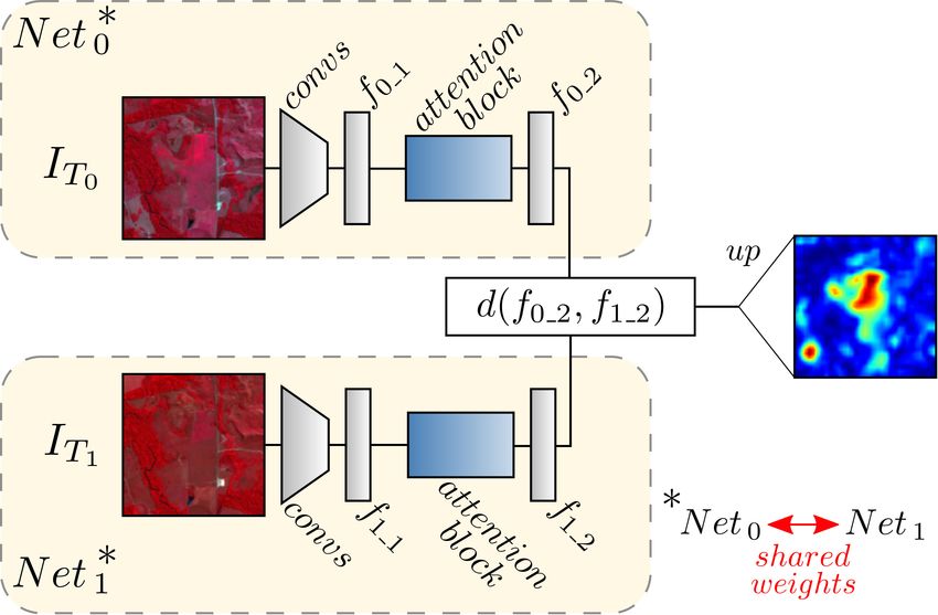
m1 . July 2018 and July 2019. For this study, we defined three
classes: 1) non-deforested areas, 2) deforested areas from July-
As mentioned before, the Contrastive Loss is a special case of
2018 to July-2019, and 3) past deforestation and borders of cur-
the WDMC Loss, where w1 and w2 assume unit value, and m1
rent deforestation. Pixels annotated with this last class shall not
is set to zero. Note that, in this case, even very similar pairs
be considered in the loss function, as they represent an over-
(small L2 distance) would still imply a positive loss, such that
all unknown class for deforestation. These classes are shown
the algorithm is slightly more prone to overfit to the training
in Figure 3 a), where blue regions denote non-deforested areas,
set. The inclusion of a margin m1 greater than zero alleviates
white regions correspond to deforested areas, and red regions
the similarity requirement, which might help in the process’s
represent past deforestation or current deforestation borders.
generalisation.
4.2 Experimental Setup
4. EXPERIMENTS
To build the training, validation and test sets, we split the data-
A series of experiments were investigated to evaluate the per- base images into 18 tiles, as shown in Figure 3 a). Given the
formance of both WDMC loss and AM applied to deforestation lack of available databases with annotation for deforestation de-
detection in a region of the Amazon rainforest. We start this tection, we partition these tiles as follows. Seven tiles were ran-
section by describing the study area to evaluate the algorithm domly selected for training, two tiles for validation, and the re-
in section 4.1. Next, in section 4.3, we examine the importance maining nine tiles for testing, resulting in a proportion 7 : 2 : 9.
of selecting proper margins in the WDMC Loss function and We selected patches of size (128 × 128) for each training tile,
how they affect the predictions of deforestation. The relevance provided that each patch contains at least 2% of deforestation
of weights in the loss function is evaluated in section 4.4. Last, (class 2). This condition was required to build a training set
we analyse the effects of AM in section 4.5. with a significant portion of deforested areas. Four examples
of training patches are shown in Figure 3 b), where the first
4.1 Study Area column contains the reference, and the second/third columns
show patches from 2018/2019 images, respectively. Note that
The study area corresponds to a region of the Amazon rainforest
located in the Pará State, Brazil. This region is centered on co- 1 https://earthexplorer.usgs.gov/
This contribution has been peer-reviewed.
https://doi.org/10.5194/isprs-archives-XLIII-B3-2021-851-2021 | © Author(s) 2021. CC BY 4.0 License. 854The International Archives of the Photogrammetry, Remote Sensing and Spatial Information Sciences, Volume XLIII-B3-2021
XXIV ISPRS Congress (2021 edition)
m2 = 2.0 m2 = 2.5
0.94 0.94
mAP
mAP
0.92 0.92
0.90 Double Margin 0.90 Double Margin
Single Margin Single Margin
0.88 0.88
0.3 0.6 0.9 1.2 1.5 0.3 0.6 0.9 1.2 1.5
m1 m1
m2 = 3.0 m2 = 3.5
0.94 0.94
mAP
mAP
0.92 0.92
0.90 Double Margin 0.90 Double Margin
Single Margin Single Margin
0.88 0.88
0.3 0.6 0.9 1.2 1.5 0.3 0.6 0.9 1.2 1.5
m1 m1
Figure 4. Analysis of mean Average Precision for different
margins used in the WDMC loss function. Dashed lines indicate
Figure 3. Overview of dataset used in the experiments. In a), a reference for m1 = 0.
Reference of Amazon deforestation between 2018 and 2019.
Blue color represents non-deforested areas, white color
represents deforested areas, and red color indicates past to the point where the distance is equal to zero. Also, it is evid-
deforested areas and current deforestation borders. In b), four ent that whenever m1 starts getting closer to m2 , it becomes
examples of patches used in training phase; from left to right: difficult to distinguish between changed and unchanged pairs.
label, image in 2018 and image in 2019, both represented in the For instance, when m2 = 2.0 and m1 = 1.5, the gap between
NIR-G-B composition. margins narrows down to 0.5, and we obtained the worst mAP,
88.74%.
although image patches are presented in Figure 3 b) NIR-G-B Given the results obtained with this experiment, in the follow-
composition, all seven bands were used in the training, valida- ing sections we kept margins m1 and m2 fixed at 0.3 and 3.0,
tion and test phases. respectively, as they provided the best mAP of 94.43%.
4.4 Dataset Imbalance Compensation
For the selected training patches, a data augmentation pro-
cedure was applied, including random rotations and hori- An assessment of the relevance of weights in the WDMC Loss
zontal/vertical flip, resulting in a total of 1704 patches for train- function is done in a similar fashion. Ten cases were evaluated
ing. in this experiment, where values of w1 ranged from 0.05 to 0.50
in steps of 0.05, while w2 is simply its compliment, i.e., w2 =
4.3 Single Margin vs Double Margin 1 − w1 . The used distance function was again the L2 norm, no
attention mechanisms were applied, and margins remain fixed
To assess the relevance of margins selection in the WDMC loss for all cases. Figure 5 displays experimental results, where the
function, the following experiment was set. We trained a net- mAP obtained in the previous section for w1 = 0.18 and w2 =
work without attention mechanisms for four values of m2 , 2.0, 0.82 is shown in blue color.
2.5, 3.0 and 3.5, and for each of these values, we evaluated the
mean Average Precision (mAP) on the test set for six different For relations w2 /w1 closer to unity, the predictions showed a
m1 ’s. One of these six values was zero, denoting a single mar- worse mAP. In contrast, relations closer to the optimal theor-
gin case. The weights w1 and w2 were maintained fixed at 0.18 etical value (Chen et al., 2020), which weights changed and
and 0.82, respectively, for all scenarios. These values represent
the proportion of deforested (18%) and not-deforested (82%) 0.944
areas in the training patches. For the distance function d(·, ·),
we chose to use the L2 norm, as it provided the best results in 0.943
(Chen et al., 2020). Figure 4 displays the experimental results.
0.942
mAP
In the four different cases evaluated in Figure 4, values of m1
0.941
closer to 0 resulted in an mAP very similar to the Single Mar-
gin case, i.e., when m1 is set to zero. This result indicates that 0.940
small variations of margins have little impact on the prediction
result. However, it is interesting to note that there was a value 0.939
of m1 > 0 that outperformed the Single Margin condition in 0.0 2.5 5.0 7.5 10.0 12.5 15.0 17.5 20.0
w1/w2
all four cases. After reaching this best-case scenario, any in-
crease in m1 tends to decrease the mAP. Although the mAP Figure 5. Analysis of mean Average Precision for different
improvement reached a maximum value less than 1% above the weights relations used in the WDMC loss function. Blue marker
Single Margin case for m2 = 2.5 and m1 = 0.3, this beha- indicates the weights relation calculated based on the proportion
viour indicates that when using a single margin, the network of changed and unchanged pixels.
might be overfitting when trying to approximate similar pairs
This contribution has been peer-reviewed.
https://doi.org/10.5194/isprs-archives-XLIII-B3-2021-851-2021 | © Author(s) 2021. CC BY 4.0 License. 855The International Archives of the Photogrammetry, Remote Sensing and Spatial Information Sciences, Volume XLIII-B3-2021
XXIV ISPRS Congress (2021 edition)
unchanged pixels according to their proportion in the dataset, We believe one of the following factors is the dominant reason
provided the best results. We can also observe that by increas- for this result: the usage of convolution operations in the SAM
ing the relevance of deforested areas even further, using a re- method might better resolve complex features, or spatial rela-
lation much greater than the theoretical optimal, the mAP de- tions are indeed more relevant than channels’ for deforestation
creases. Last, it is relevant to highlight the difference in mAP detection. Further analysis needs to be done before asserting
between a poorly set pair of weights and the best-case scenario, which is the prevailing factor.
which was found to be 0.52% according to Figure 5.
Also, according to Table 1, the CAM method did not provide
4.5 Effects of Attention Mechanisms many improvements compared to the baseline method. How-
ever, when combining CAM with SAM, nearly all metrics
An analysis of the effects of AM on deforestation detection is showed an improvement compared to the SAM method isol-
provided in this section. In contrast to the previous sections, ated. The best mAP obtained was for the dual-attention method,
where the experiments considered modifications only in the loss with an increase of 1.06% compared to the baseline method.
function, here, we implemented modifications in the network
architecture to evaluate the contribution of each AM separately.
Four methods were considered: (I) a baseline (BL) architec- 5. CONCLUSIONS
ture without AM, with the distance function applied directly to
the feature embeddings f0 1 and f1 1 ; (II) an architecture with This paper reported the application of a deep-learning network,
only a CAM present in the attention block; (III) another with equipped with a dual-attention mechanism, to the task of de-
only a SAM present; and (IV) with the dual-attention mechan- forestation detection in the Amazon rainforest. A recently pro-
isms combined. Weights w1 and w2 of WDMC loss function posed loss function, the WDMC loss, was used throughout the
were kept fixed and equal to 0.1 and 0.9, respectively, as these work. A set of experiments were implemented to analyse the
provided the best mAP in the previous section, equal to 94.44%. effects of both margins and weights of the WDMC loss function
in the prediction of deforestation. Results suggest that adding
Visual results for deforestation predictions of networks trained a second margin to the classic contrastive loss function might
with these four strategies are shown in Figure 6. There, five ex- bring benefits in terms of generalisation, as it can help avoid
amples are provided, each presented in a single row. The first overfitting. Also, it was shown that the weights of the loss func-
three columns show an input test patch from the 2018 image, its tion could impact the mean average precision of deforestation
co-registered pair from 2019, and the ground truth (GT). The detection in up to 0.52%.
last four columns present the change map results from the four
methods evaluated (I)-(IV), respectively. Blue colour represents Further experiments were developed to investigate the effects
the zero probability of deforestation class and red the maximum of self-attention mechanisms in deforestation detection. Res-
probability. For instance, the first row shows that architectures ults showed that the spatial content of images was more rel-
using the dual-attention modules distinguish the deforested re- evant for attention mechanism than the channel content. The
gions accurately, providing more confident outputs and resolv- usage of a spatial attention mechanism resulted in an improve-
ing complex geometries in a better way. On the other hand, the ment in mean average precision of 0.71%, and when combined
BL architecture presented more false-positive regions, classi- with channel attention mechanism, the improvement increased
fying the class past deforestation as deforestation. The CAM to 1.06%. To our best knowledge, this is the first work that
and SAM outputs deliver fewer false-positive regions, but they reports an analysis of dual-attention mechanisms with WDMC
produced less confident values than the dual-attention mechan- loss function applied to deforestation detection. Thus, given the
isms. consistent improvements in predicting deforestation, we believe
Any further analysis requires a comparison of metrics to eval- this work might encourage other researchers in the challenging
uate the performance of each method. For this reason, we task of deforestation detection.
provide a plot related to precision and recall scores for the four
evaluated methods (see Figure 7). Furthermore, Table 1 sum- 6. ACKNOWLEDGEMENTS
marises the numerical results in terms of Recall, Precision, F1-
score (F1), and mAP. By carefully analysing the result in Fig-
ure 7, we can see an increase in the prediction performance Authors would like to thank Conselho Nacional de Desen-
when SAM is employed. The SAM method and dual-attention volvimento Cientı́fico e Tecnológico (CNPq), Coordenação de
method curves lie above the CAM and baseline curves for all Aperfeiçoamento de Pessoal de Nı́vel Superior (CAPES) and
recall values. Fundação de Amparo à Pesquisa do Estado do Rio de Janeiro
(FAPERJ) for the financial support.
Method Rec. Prec. F1 mAP
Baseline 93.00 81.44 86.83 94.44
CAM 94.91 80.16 86.91 94.49 REFERENCES
SAM 94.28 80.80 87.02 95.15
SAM + CAM 93.99 81.62 87.36 95.50 Asokan, A., Anitha, J., 2019. Change detection techniques for
remote sensing applications: a survey. Earth Science Informat-
Table 1. Metrics results, in [%], for the four methods evaluated. ics, 12, 143–160.
Since there are a few crosses between the curves of CAM and Assis, F., Fernando, L., Ferreira, K. R., Vinhas, L., Maurano, L.,
baseline methods and between SAM and dual-attention meth- Almeida, C., Carvalho, A., Rodrigues, J., Maciel, A., Camargo,
ods, we must analyse metrics results numerically to further con- C., 2019. TerraBrasilis: A Spatial Data Analytics Infrastruc-
clusions. Table 1 shows that methods using spatial attention ture for Large-Scale Thematic Mapping. ISPRS International
mechanisms indeed outperformed CAM and baseline methods. Journal of Geo-Information, 8(11), 513.
This contribution has been peer-reviewed.
https://doi.org/10.5194/isprs-archives-XLIII-B3-2021-851-2021 | © Author(s) 2021. CC BY 4.0 License. 856The International Archives of the Photogrammetry, Remote Sensing and Spatial Information Sciences, Volume XLIII-B3-2021
XXIV ISPRS Congress (2021 edition)
Figure 6. Visual results for the four methods evaluated. Each row presents an example of test patch assessed, and columns, from left to
right, are: input image patch taken in 2018; input image patch taken in 2019; ground truth; and the change maps of baseline method;
CAM; SAM; and dual-attention method.
line Deforestation Monitoring in Chaco Forest. IEEE Transac-
tions on Geoscience and Remote Sensing, 58(2), 1303-1312.
Guo, T., Wang, D., Jiang, Z., Men, A., Zhou, Y., 2018.
Deep network with spatial and channel attention for person re-
3UHFLVLRQ
identification. 2018 IEEE Visual Communications and Image
Processing (VCIP), 1–4.
%DVHOLQH
&$0 Hadsell, R., Chopra, S., LeCun, Y., 2006. Dimensionality re-
duction by learning an invariant mapping. 2006 IEEE Computer
6$0
Society Conference on Computer Vision and Pattern Recogni-
6$0&$0 tion (CVPR’06), 2, 1735–1742.
5HFDOO Hecheltjen, A., Thonfeld, F., Menz, G., 2014. Recent Advances
in Remote Sensing Change Detection – A Review. Springer
Figure 7. Relation between precision and recall for the four Netherlands, 145–178.
methods evaluated.
Hu, J., Shen, L., Sun, G., 2018. Squeeze-and-excitation net-
works. 2018 IEEE/CVF Conference on Computer Vision and
Bahdanau, D., Cho, K., Bengio, Y., 2015. Neural Machine Pattern Recognition, 7132–7141.
Translation by Jointly Learning to Align and Translate. CoRR,
abs/1409.0473. INPE, 2020. Monitoring of the brazilian amazo-
nian forest by satellite. Available online:
Barlow, J., Lennox, G. D., Gardner, T. A., 2016. Anthropogenic http://www.obt.inpe.br/OBT/assuntos/programas/amazonia/prodes
disturbance in tropical forests can double biodiversity loss from (accessed on 29 November 2020).
deforestation. Nature, 535, 144-147.
Lean, J., Warrilow, D. A., 1989. Simulation of the regional cli-
matic impact of Amazon deforestation. Nature, 342, 411–413.
Chen, J., Yuan, Z., Peng, J., Chen, L., Haozhe, H., Zhu, J., Liu,
Y., Li, H., 2020. DASNet: Dual attentive fully convolutional Lee, S.-H., Han, K.-J., Lee, K., Lee, K.-J., Oh, K.-Y., Lee, M.-
siamese networks for change detection of high resolution satel- J., 2020. Classification of Landscape Affected by Deforesta-
lite images. IEEE Journal of Selected Topics in Applied Earth tion Using High-Resolution Remote Sensing Data and Deep-
Observations and Remote Sensing, 1-1. Learning Techniques. Remote Sensing, 12(20).
de Bem, P. P., de Carvalho Junior, O. A., Fontes Guimarães, Li, F., Bai, H., Zhao, Y., 2020. Learning a Deep Dual Atten-
R., Trancoso Gomes, R. A., 2020. Change Detection of De- tion Network for Video Super-Resolution. IEEE Transactions
forestation in the Brazilian Amazon Using Landsat Data and on Image Processing, 29, 4474-4488.
Convolutional Neural Networks. Remote Sensing, 12(6).
Lu, D., Mausel, P., Brondı́zio, E., Moran, E., 2004. Change
Grings, F., Roitberg, E., Barraza, V., 2020. EVI Time-Series detection techniques. International Journal of Remote Sensing,
Breakpoint Detection Using Convolutional Networks for On- 25(12), 2365-2401.
This contribution has been peer-reviewed.
https://doi.org/10.5194/isprs-archives-XLIII-B3-2021-851-2021 | © Author(s) 2021. CC BY 4.0 License. 857The International Archives of the Photogrammetry, Remote Sensing and Spatial Information Sciences, Volume XLIII-B3-2021
XXIV ISPRS Congress (2021 edition)
MacDonald, A. J., Mordecai, E. A., 2019. Amazon deforest-
ation drives malaria transmission, and malaria burden reduces
forest clearing. Proceedings of the National Academy of Sci-
ences, 116(44), 22212–22218.
Mahayossanunt, Y., Thannamitsomboon, T., Keatmanee, C.,
2019. Convolutional neural network and attention mechanism
for bone age prediction. 2019 IEEE Asia Pacific Conference on
Circuits and Systems (APCCAS), 249–252.
Maretto, R. V., Fonseca, L. M. G., Jacobs, N., Körting, T. S.,
Bendini, H. N., Parente, L. L., 2020. Spatio-Temporal Deep
Learning Approach to Map Deforestation in Amazon Rain-
forest. IEEE Geoscience and Remote Sensing Letters, 1-5.
Medvigy, D., Walko, R. L., Otte, M. J., Avissar, R., 2013.
Simulated Changes in Northwest U.S. Climate in Response
to Amazon Deforestation*. Journal of Climate, 26(22), 9115-
9136.
Ortega Adarme, M., Queiroz Feitosa, R., Nigri Happ, P., Apare-
cido De Almeida, C., Rodrigues Gomes, A., 2020. Evaluation
of Deep Learning Techniques for Deforestation Detection in the
Brazilian Amazon and Cerrado Biomes From Remote Sensing
Imagery. Remote Sensing, 12(6).
Ramachandran, P., Parmar, N., Vaswani, A., Bello, I.,
Levskaya, A., Shlens, J., 2019. Stand-alone self-attention in
vision models. H. Wallach, H. Larochelle, A. Beygelzimer,
F. d'Alché-Buc, E. Fox, R. Garnett (eds), Advances in Neural
Information Processing Systems, 32, Curran Associates, Inc.,
68–80.
Roy, A. G., Navab, N., Wachinger, C., 2019. Recalibrat-
ing Fully Convolutional Networks With Spatial and Channel
“Squeeze and Excitation” Blocks. IEEE Transactions on Med-
ical Imaging, 38(2), 540-549.
Shukla, J., Nobre, C., Sellers, P., 1990. Amazon Deforestation
and Climate Change. Science, 247(4948), 1322–1325.
Swann, A. L., Longo, M., Knox, R. G., Lee, E., Moorcroft,
P. R., 2015. Future deforestation in the Amazon and con-
sequences for South American climate. Agricultural and Forest
Meteorology, 214-215, 12 - 24.
Sy, V. D., Herold, M., Achard, F., Beuchle, R., Clevers, J. G.
P. W., Lindquist, E., Verchot, L., 2015. Land use patterns and
related carbon losses following deforestation in South America.
Environmental Research Letters, 10(12), 124004.
Wiemker, R., 1997. An iterative spectral-spatial bayesian la-
beling approach for unsupervised robust change detection on re-
motely sensed multispectral imagery. G. Sommer, K. Daniilidis,
J. Pauli (eds), Computer Analysis of Images and Patterns,
Springer Berlin Heidelberg, Berlin, Heidelberg, 263–270.
Xu, B., Liu, J., Hou, X., Liu, B., Garibaldi, J., Ellis, I. O.,
Green, A., Shen, L., Qiu, G., 2019. Look, investigate, and clas-
sify: A deep hybrid attention method for breast cancer classific-
ation. 2019 IEEE 16th International Symposium on Biomedical
Imaging (ISBI 2019), 914–918.
This contribution has been peer-reviewed.
https://doi.org/10.5194/isprs-archives-XLIII-B3-2021-851-2021 | © Author(s) 2021. CC BY 4.0 License. 858You can also read