Detection of a 14-days atmospheric perturbation peak at Paranal associated with lunar cycles
←
→
Page content transcription
If your browser does not render page correctly, please read the page content below
Mon. Not. R. Astron. Soc. 000, 1–5 (2009) Printed 21 February 2019 (MN LATEX style file v2.2)
Detection of a 14-days atmospheric perturbation peak at
Paranal associated with lunar cycles
S. Cavazzani1,2⋆ , S. Ortolani1,2, N. Scafetta3, V. Zitelli 4 , G. Carraro1
arXiv:1902.07339v1 [astro-ph.IM] 19 Feb 2019
1 Department of Physics and Astronomy, University of Padova, Vicolo dell’Osservatorio 3, 35122, Padova, Italy
2 INAF-Osservatorio Astronomico di Padova, Vicolo dell’Osservatorio 5, 35122, Padova, Italy
3 Dipartimento di Scienze della Terra, dell’Ambiente e delle Risorse, University of Naples, Via Cinthia 21, 80126, Naples, Italy
4 INAF-OAS Osservatorio di Astrofisica e Scienza dello Spazio di Bologna, Via Gobetti 93/3, 40129, Bologna, Italy
Accepted 0000 September 00. Received 0000 September 00; in original form 0000 May 00.
ABSTRACT
In this paper we investigate the correlation between the atmospheric perturbations
at Paranal Observatory and the Chilean coast tides, which are mostly modulated by
the 14-day syzygy solar-lunar tidal cycle. To this aim, we downloaded 15 years (2003-
2017) of cloud coverage data from the AQUA satellite, in a matrix that includes also
Armazones, the site of the European Extremely Large Telescope. By applying the
Fast Fourier Transform to these data we detected a periodicity peak of about 14 days.
We studied the tide cycle at Chanaral De Las Animas, on the ocean coast, for the
year 2017, and we correlated it with the atmospheric perturbations at Paranal and
the lunar phases. We found a significant correlation (96%) between the phenomena of
short duration and intensity (1-3 days) and the tidal cycle at Chanaral. We then show
that an atmospheric perturbation occurs at Paranal in concomitance with the low tide,
which anticipates the full (or the new) moon by 3-4 days. This result allows to improve
current weather forecasting models for astronomical observatories by introducing a
lunar variable.
Key words: atmospheric effects – optical turbulence – tidal atmospheric influence.
1 INTRODUCTION zani et al. (2015), and Osborn et al. (2018). On the other
hand, the availability of longer term data from satellites
Reliable predictions of the observational conditions at as-
permits a statistical approach and the search for periodic
tronomical sites, especially the degree of cloud coverage,
trends. In this paper we show an analysis of long term fore-
are a crucial ingredient for modern astronomical observa-
cast making use of the Cerro Paranal Observatory environ-
tions. The widespread use of adaptive optics in particular is
mental data for a detailed temporal analysis of atmospheric
very sensitive to the cloud coverage conditions (as well as to
perturbations, including cloud cover, strong wind, high hu-
strong wind and seeing conditions) for a proper operation.
midity, and bad seeing conditions. The model proposed in
Both the optimisation of the resources and the observational
this paper correlates moon phases, tides and atmospheric
scheduling program require the statistics of clear/mixed or
perturbations to forecast observing required conditions on
covered time and its yearly, monthly or shorter time dis-
long and short terms. In particular, we seek empirical con-
tribution. In addition, recent requests for optical commu-
firmations of a possible lunisolar tidal modulation of mete-
nications for astronomical applications (with satellites or
orological parameters, which has been the subject of lively
between distant telescopes) make the cloud coverage pre-
debate (Crawford, 1982, Lakshmi et al., 1998, and Hagan et
dictions more relevant. Generally speaking, there are two
al., 2003). We analysed a 15 year database of cloud cover
approaches to this issue. One consists in the short time fore-
at Paranal (2003-2017) from the MODIS (Moderate Resolu-
cast which predicts the cloud coverage level up to a few days,
tion Imaging Spectro-radiometer) instrument (bands 27 to
while the other is based on the statistical analysis of longer
36) onboard the AQUA polar satellite. We applied the fast
term trends. Example of short time forecasts of observing
Fourier transform (FFT) to these data as in Cavazzani et al.
conditions (including wind and turbulence) are in Masciadri
(2017). A sharp periodicity of 178 ± 7 days is found, being
et al. (2002), Sarazin (2005), Giordano et al. (2013), Cavaz-
June and December the most perturbed months. We looked
for shorter periodicities of the first harmonic, and the FFT
analysis returned a periodicity of 14.0 ± 0.5 days of weaker
⋆ E-mail:stefano.cavazzani@unipd.it
c 2009 RAS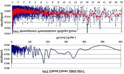
2 S. Cavazzani et al.
Figure 1. Location of the analyzed sites, the matrix 1◦ × 1◦
used for the analysis of atmospheric perturbations and pressure
contains both sites: Paranal (LAT. −24◦ 37′ , LONG. −70◦ 24′ , Al-
titude 2635 m) and Armazones (LAT. −24◦ 35′ , LONG. −70◦ 11′ ,
Altitude 3064 m). Chanaral De Las Animas (LAT. −26◦ 20′ ,
LONG. −70◦ 36′ , Altitude 198 m) was used for the oceanic tides
analysis.
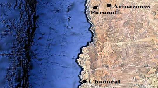
Figure 3. (Top panel) FFT of the atmospheric perturbations
(2003-2017 night MODIS data): main annual and semiannual pe-
riods. (Central panel) FFT high-frequency zoom (blue) with its
7-point moving average curve (red): the highest 14-days peak
is highlighted. (Bottom panel) FFT of the pressure record at
Paranal (2003-2017): main annual and semiannual periods.
2 DATA ANALYSIS AND ERROR BUDGET
Following Cavazzani et al. (2017) we have applied the Fast
Fourier Transform (FFT) to the cloud cover data (top panel)
and the pressure data (bottom panel) at Paranal (2003-
2017) presented in Fig. 2 as 28-day monthly averages from
MODIS. Fig. 3 shows the respective FFT trend after the
conversion of the main frequencies in main periods (Cooley-
Tukey, 1965). We can see that we have a strong perturbation
every 178 days corresponding to about half year (top panel).
Figure 2. Top panel shows the cloud coverage trend at Paranal,
bottom panel shows the pressure trend at Paranal during the The error analysis on the period of this peak is provided in
same period. Time is in Julian days (JD): 2450000 + 2640 (x- three independent ways allowing a triple check of the va-
axis). lidity of the results. The first analysis is based on the error
propagation and provides us with the maximum error due to
data sampling. Through the propagation formula described
in Cavazzani et al. (2017) we get a maximum error of 4%,
atmospheric perturbations. This perturbation is most prob- which corresponds to an uncertainty of ±7 days. The sec-
ably related to the 14-day luni-solar cycle (full moon and ond error estimate is based on the frequency resolution of
new moon). We then analysed the same Paranal database the Fourier analysis defined as ∇f = 1/T = fP /N , where T
for pressure trends, to search for physical explanations. The is the period, fP is the frequency of the peak and N is the
data are provided by the GLDAS Model (GLDAS datasets data population. A frequency fP associated with a spectral
are available from the NASA Goddard Earth Sciences Data peak has an uncertainty of ± 12 ∇f and the correspondent
and Information Services Center (GES DISC). They give period P is:
daily values for 1◦ × 1◦ areas, like those of cloud cover data. 1 1 ∇f 1 P2
To this aim, we added the ocean tides at Chanaral De Las P = 1
= ± 2 = ± (1)
f∓ 2
∇f f 2f f 2T
Animas (see Fig. 1) database, and performed a triple cor-
relation: atmospheric perturbations - lunar cycles - oceanic From this formula we derive an uncertainty of ±4 days
tides. Fig. 1 shows the geographic area of interest and lists on the semiannual period. This result is consistent with the
the characteristics of the various sites. The layout of the pa- full width at half maximum (FWHM) of the analyzed peak.
per is as follows. In Section 2 we briefly describe the Fourier The zoom in the top panel shows a FWHM of 10 days
Transform (FT) and in particular the Fast Fourier Trans- (hence, ±5 days). Thus, the uncertainty on the frequency
form (FFT) used in this analysis. Section 3 is devoted to resolution (±4 days) and the FWHM (±5 days) have a differ-
the analysis of the correlation between atmospheric pertur- ence of one day only. We believe that the most reliable error
bations, oceanic tides and lunar cycles. Section 4, finally, to be associated with the peak of 178 days is the maximum
discusses the results and draws some conclusions. error due to the error propagation (±7), which makes the
c 2009 RAS, MNRAS 000, 1–5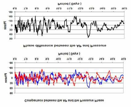
Site Testing         3
peak compatible with a semiannual cycle. The FFT spectra
shown in Fig. 3 also suggest the presence of minor oscilla-
tions with periods of about 206 and 412 days, which are also
observed among the long-range oceanic tides (Avsyuk and
Maslov, 2011). Central panel of Fig. 3 shows the 20-days
FFT high-frequency zoom (blue) with its 7-point moving
average curve (red). This signal is correlated with the at-
mospheric perturbations (AP) at Paranal (Cavazzani et al.,
2017). Fig. 4 shows FFT 7-points moving average spectra for
the periods between 13.25 and 15.25 days (top panel). The
main period of a perturbation at Paranal is about 14 days.
Thus, there is a higher probability to have a covered night
every two weeks: a fact that is validated by consulting the
Paranal ground data on environmental monitoring1 . We did
the same analysis with the pressure data at Paranal during
the same period, as provided by the GLDAS Model. Bottom
panel of Fig. 3 shows main semiannual and annual main pe-
riod peaks in full agreement with the cloud cover results.
The bottom panel of Fig. 4 shows a zoom of the FFT dur-
ing the periods between 13.25 and 15.25 days: we have two         Figure 4. Comparison between the cloud cover periodicity and
periodicities. This perturbation is most probably related to      the periodicity of the pressure variation at Paranal. Top panel
the first harmonic of the tropical and synodical lunar months     shows the zoom of the atmospheric perturbations peak with its
generating the lunisolar fortnightly (Mf ) tide (period, 13.7     associated FWHM. Bottom panel shows the zoom of the pressure
days) and the lunisolar synodic fortnightly (Msf ) tide (pe-      peaks.
riod, 14.6-15.0 days). In order to strengthen our findings, we
calculated the error associated with the 14-day peak in three
different ways: a maximum error of 4.0% which corresponds         the tide. The results of a FFT run on the tide data are shown
to 13 hours and 26 minutes through the error propagation          in Fig. 6 (top panel). Very interestingly, one can clearly spot
due to satellite data; an error of 2.4% by applying the equa-     both the 14-day periodicity correlated with the lunar cycle
tion 1 which corresponds to 8 hours and 10 minutes and the        and the 14-day oscillation of the atmospheric perturbations.
0.7-day FWHM of the 14-day peak corresponds to an error           The phases of the two fluctuations are calculated and com-
of 2.5% (8 hours and 24 minutes). In summary we have ob-          pared in the central panel of Fig. 6. We noted that at the
tained the following results: 14 ± 0.56 days with the error       period of 14 days the tide phase is −60 degrees compared
propagation, 14 ± 0.34 days with the frequency resolution of      against the atmospheric perturbation phase, which trans-
the Fourier analysis, and 14 ± 0.35 days with the FWHM of         lates into 2 days and 8 hours delay. To cast more light on
the 14-day peak (see Fig. 4). This confirms the validity of       this evidence, we show in Fig. 7 the trend of these data for
the analysis. The error on the amplitude of the peaks can be      January and February 2017. Atmospheric conditions data
calculated through the formula ∆ = σ 2 /T , where σ is the        are taken from Paranal web page. Over this period the tide
statistical error of the satellite data and T is the analyzed     maximum varies between 1.2 m and 1.8 m. The low tide
period. Even if we consider a maximum error on the data of        anticipates the full moon or the new moon of about three
10 percent and a period of 15 years (about 365 x 15 days) we      days. A tight correlation seems to exists between the low
obtain an amplitude error of about ±1.8 · 10−4 which is neg-      tide (and hence moon) cycle and the atmospheric perturba-
ligible compared to those previously calculated. Finally, we      tions (indicated by blue clouds). Fig. 7 shows four different
compared the phases of the two oscillations in Fig. 5, which      bad condition occurrences: on Jan 23 intense clouds and bad
shows the phase of atmospheric perturbations (continuous          seeing, on Feb 8 clouds, seeing worsening and high precip-
blue) and the phase of pressure oscillations (dasched red),       itable water vapor (PWW), and on Jan 10 and Feb 22 thick
and again we note that the two oscillations are in phase on       clouds and bad seeing. We can see that the first two per-
the 14th day.                                                     turbations are separated by about 15 days, while the third
                                                                  is separated exactly by 14 days from the second. Besides,
                                                                  all perturbations occur at low tide. Bottom panel shows the
                                                                  same trend for 2017 April, May and June. We can see 5 per-
3     CORRELATION BETWEEN ATMOSPHERIC
                                                                  turbations more in relation to the tides and the lunar cycle.
      PERTURBATIONS, OCEANIC TIDES AND
                                                                  When extended to the whole years, this analysis yields a
      LUNAR CYCLES
                                                                  mean correlation as large as 96%. Table 1 summarises the
In this Section we correlate the meteorological results with      results of the correlation. Column 2 shows the correlation
the ocean tides at Chanaral de las Animas (see Fig. 1) and        between the atmospheric perturbations (AP) and the lunar
the underlying lunar cycles. We extract from the 2017 tide        cycles (LC): Fourier analysis shows that the AP anticipates
database (Tides Planner app2 ) the daily maximum value of         the full moon or the new moon by 2 days and 8 hours. We
                                                                  considered the AP of January and analyzed the LC. If the
                                                                  perturbations occur with a temporal shift respect to the fore-
1   http://archive.eso.org/cms/eso-data/ambient-conditions.html   cast the correlation decreases, i.e. we have about 2 perturba-
2   https://www.imray.com/tides-planner-app/                      tions every month. If these occur exactly 2 days and 8 hours

c 2009 RAS, MNRAS 000, 1–5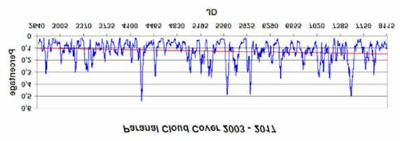
4 S. Cavazzani et al.
Figure 5. Comparison between the phase of atmospheric pertur-
bations (continuous blue) and the phase of pressure oscillations
(dashed red), the two oscillations are in phase on the 14th day.
before the full or new moon the correlation is 100 percent. A
3 percent error on a 31-day month corresponds to about 22
hours: this means that one perturbation can be anticipated
or delayed by about one day, or both anticipate or delay by
about 10 hours. The same procedure was applied between
the AP and the oceanic tides (OT) and between LC and OT
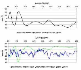
columns 3 and 4 respectively. We emphasize that our model Figure 6. Top panel shows the FFT of the tides in Chanaral De
is not aimed at an hourly precision: the model allows to Las Animas in 2017, central panel shows the comparison between
forecast observation periods with a high probability of clear the phase of atmospheric perturbations (continuous blue line) and
the phase of the tides (dashed green line) and bottom panel shows
and stable atmospheric conditions with a long time horizon
the phase difference.
based on the moon phases. At Chanaral de las Animas the
minimum tide occurs between 5 pm and 7 pm (local time)
during the days with atmospheric perturbations. This would
take away superficial water from the ribs after the hot daily
hours, consequently the coasts get cooler because the cold
water rises from the depth and the temperature decreases
would favour cloud formation or worsening of seeing. Fried and from August to October (see Fig. 8, right panel). This
(1965) showed that seeing is related to the integral of Cn2 result is very useful for the long-term observational program
(refractive index structure parameter). In turn, Cn2 is linked scheduling. The solar-lunar tidal effects on the oceanic cur-
to CT2 (temperature structure parameter) and therefore to rents, as well as on meteorology (Hagan et al., 2003), have
the temperature variations. been extensively discussed in the literature. Currie (1983)
identified a periodic (18.6 years) nodal-induced drought in
the Patagonian Andes. This 18.6 year cycle modulates the
monthly and semi-monthly tidal cycles. Moreover, a 27.3
4 DISCUSSION AND CONCLUSION
and 13.6 day cycles (produced by to solar-lunar tidal field)
In this paper we identified a weather perturbation at Cerro modulates the atmospheric circulation producing changes in
Paranal on a ∼14 days cycle which seems to be strongly zonal wind velocity (Li, 2005). A tidal forcing of the polar
correlated with the Mf and Msf solar-lunar tidal cycles. jet stream with periods of about 14 and 28 days tidal cycles
In detail, we found that the cloud cover degree at Cerro has been recently observed (Best and Madrigali, 2016). Fi-
Paranal increases during the low ocean tidal cycle on the nally, in Shinsuke et al. (2015) a relationship is established
Chilean coast at about 25 S latitude (see Fig 1). This hap- between the 14-days cycle, the ocean temperatures, and the
pens close to the Waxing Gibbons (WB) and the Waning wind speed in Japan. A possible physical explanation could
Crescent (WC) lunar phases that occur 3-4 days before the be that on the Chilean coasts the Humboldt current com-
new or full moon, respectively (see Fig. 8). These perturba- bined with the tidal cycle activates a quasi 14-days recur-
tions normally last about one or two nights when the seeing rence of ocean water transport. At Chanaral de las Animas
index is larger than 1 arcsec. On the contrary, between the the minimum of low tide occurs in the late afternoon dur-
two perturbations periods the sky is normally clear with ing the lunar phases of WG and WC. This dynamic favors
a seeing index smaller than 1 arcsec. This correlation varies the formation of thermal inhomogeneities along the Chilean
with the season (see Table 1) and is maximum in October. In coast and therefore a weather pertubation on the Andes.
general, the model accuracy is higher from February to April This hypothesys could be tested in a following work.
c 2009 RAS, MNRAS 000, 1–5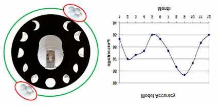
Site Testing         5

                                                                     Figure 8. Left panel shows the lunar clock for the atmospheric
                                                                     perturbations forecast: at the top we see the perturbation during
                                                                     the Waxing Gibbons (WG) before the full moon while below we
                                                                     see the perturbation during the Waning Crescent (WC) before the
                                                                     new moon. The period between the two perturbations is stable
                                                                     with seeing smaller than 1 arcsec. Right panel shows the 3-month
                                                                     moving average for the accuracy of the model.

                                                                     REFERENCES
Figure 7. Tide maximum varies between 1.2m and 1.8m at Cha-
naral de las Animas, the low tide anticipates the full moon or the    Avsyuk, Y.N., Maslov, L.A., 2011, Earth Moon Planets,
new moon of about three days. The figure shows an example of           108, 77
three types of atmospheric perturbations (represented schemati-       Best, C.H. and Madrigali, R., 2016, Atmos. Chem. Phys.
cally by clouds): an intense one with clouds and high seeing on 24     Discuss., 15, 22701
January, the second one is characterized by clouds, a worsening       Cavazzani, S., Ortolani, S., Zitelli, V., 2015, MNRAS, 452,
of the seeing and a precipitable water vapor (PWW) increase on
                                                                       2185
8 February and a third intense one with clouds and high seeing
on 22 February, 2017.
                                                                      Cavazzani, S., Ortolani, S., Zitelli, V., 2017, MNRAS, 471,
                                                                       2616
                                                                      Cooley, J.W., Tukey J.W., 1965, Mathematics of Compu-
                                                                       tation, 19, 297
 Table 1. Correlation between atmospheric perturbations               Crawford, W.R., 1982, International Hydrographic Review,
 (AP) at Paranal, lunar cycles (LC) and ocean tides (OT) at
                                                                       59, 131
 Chanaral (2017). The last column is the 3-month moving av-
 erage (3-MMA).
                                                                      Currie, R.G., 1983, Geophysical Research Letters, 10, 1089
                                                                      Fried D.L., 1965, J. Opt. Soc. Am., 55, 1427
                                                                      Giordano C. et al., 2013, MNRAS, 430, 3102
 Paranal               AP-LC-OT correlations
                                                                      Hagan, M.E., Forbes, J.M. and Richmond, A., 2003, Ency-
 Month         AP-LC      AP-OT      LC-OT     Mean     3-MMA          clopedia of Atmospheric Sciences, 1, 159.
                                                                      Holton, J.R., 2004, An Introduction to Dynamic Meteo-
 January          97        97         100       98        95
 February         97        97         97        97        97          rology, Fourth Edition, Vol. 88 in the International Geo-
 March            94        94         100       96        97          physics series
 April            93        97         100       97        96         Lakshmi, H., Kantha, J., Scott S., Shailen, D.D., 1998,
 May              94        97         97        96        95          Journal of Geophysical Reserrch, 103, 12639
 June             90        90         97        92        95         Li, G., 2005, Adv. Atmos. Sci., 22, 359
 July             97        97         100       98        96         Masciadri, E., Avila, R., Sanchez, L. J., 2002, Astronomy
 August           97        100        100       99        98          and Astrophysics, 382, 378
 September        93        97         97        96        98         Osborn, J., Sarazin, M., 2018, MNRAS, 480, 1278
 October         100        100        100       100       97
                                                                      Sarazin, M., 2005, TMT Site Testing Workshop, Vancou-
 November         93        97         97        96        96
                                                                       ver.
 December         90        90         93        91        95
                                                                      Shinsuke, I., Atsuhiko, I., Yasuyuki, M., 2015, Nature, Sci-
 Mean                                            96                    entific Reports, 5, 10167

4.1   ACKNOWLEDGMENTS
This activity is supported by the INAF (Istituto Nazionale
di Astrofisica) funds allocated to the Premiale ADONI
MIUR. MODIS data were provided by the Giovanni - In-
teractive Visualization and Analysis website. We also refer
to the 3D atmospheric reconstruction project at Prato Pi-
azza (Italy). Finally we thank the support of the University
of Padua for this search (Research grant, type A, Rep. 138,
Prot. 3022, 26/10/2018).

c 2009 RAS, MNRAS 000, 1–5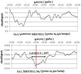
You can also read