DEVELOPING AN ALGORITHMIC TRADING BOT - Tri Nam Do - Theseus
←
→
Page content transcription
If your browser does not render page correctly, please read the page content below
Tri Nam Do

DEVELOPING AN ALGORITHMIC TRADING BOT

                             1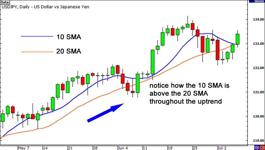
Developing an Algorithmic Trading Bot

                                        Tri Nam Do
                                        Bachelor’s Thesis
                                        Spring 2021
                                        Bachelor’s Degree in Software Engineering
                                        Oulu University of Applied Sciences

                                    2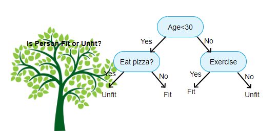
ABSTRACT

Oulu University of Applied Sciences
Bachelor’s degree in Software Engineering

Author: Tri Nam Do
Title of the thesis: Developing an algorithmic trading bot
Thesis examiner(s): Teemu Korpela
Term and year of thesis completion: Spring 2021                    Pages: 49

The idea of cloud computing was conceived a few decades ago but only until recently has it
received considerable notice from the global developer communities, particularly when made
remarkably more approachable and affordable for the SMEs and recreational developers with AWS
Free Tier and Azure free accounts. However, the big picture of how all components of a cloud
service provider work together is still quite challenging to comprehend. Therefore, the outcome
which this thesis aims to achieve is to demonstrate how the most popular services provided by
AWS can cooperate all together in an exemplary cloud application – an automated stock trading
bot.

This thesis also provides a descriptive explanation on the fundamentals of stock investing and
trading as well as some popular trading strategies, including ones with the aid of Machine Learning
models to predict the price movement of certain stocks so that readers without a background in
Investing or Data Science can follow through the reasoning of how the program was designed in a
specific way. It is widely believed that the stock price is implausible to be predicted, so this project
did not dive deep into optimizing the results but to present a suggestion as to how the use of
Machine Learning can fit in the big picture.

Overall, the result of this project was within expectation, meaning that a functional prototype of the
program was produced with the capability of further development and scaling up. This was
accomplished by setting up a logical design of the program, gradually making each of them
functional and connecting them together so they can function as a whole.

Keywords: Trading, AWS, Automation, Serverless

                                                   3
CONTENTS
CONTENTS .................................................................................................................................... 4
TERMS ........................................................................................................................................... 6
1 INTRODUCTION .................................................................................................................... 7
2 STOCK INVESTING ESSENTIALS ........................................................................................ 8
2.1 Elemental concepts ..................................................................................................... 8
2.2 Trading strategy .......................................................................................................... 9
2.2.1 Definition ....................................................................................................... 9
2.2.2 Development of a trading strategy .............................................................. 10
2.2.3 Technical indicator ...................................................................................... 10
2.2.4 Going long and going short ......................................................................... 11
2.2.5 Trading frequency ....................................................................................... 12
2.2.6 Strategies and technical indicators used in this project .............................. 12
3 PROGRAM OUTLINE........................................................................................................... 14
3.1 Topological diagram .................................................................................................. 14
3.2 Deployment infrastructure ......................................................................................... 15
3.3 Development environment ........................................................................................ 16
3.3.1 Operating system ........................................................................................ 16
3.3.2 Programming language .............................................................................. 16
3.3.3 Code editor ................................................................................................. 17
3.3.4 Project encapsulation technology ............................................................... 18
3.3.5 Version control system ............................................................................... 20
3.3.6 Database management tools ...................................................................... 20
4 DATABASE........................................................................................................................... 22
4.1 Functional requirements ............................................................................................ 22
4.2 Non-functional requirements ..................................................................................... 22
4.3 Database schema ..................................................................................................... 24
4.4 Development and deployment................................................................................... 25
4.4.1 Development phase .................................................................................... 25
4.4.2 Deployment phase ...................................................................................... 27
5 DECISION-MAKING MODULE............................................................................................. 28
5.1 Functional requirements ............................................................................................ 28
45.2 Non-functional requirements ..................................................................................... 28
5.3 Development and deployment................................................................................... 28
5.3.1 Simple Moving Average Crossover ............................................................ 29
5.3.2 Machine Learning for classification ............................................................. 31
5.3.3 Deployment phase ...................................................................................... 38
6 ORCHESTRATION MODULE .............................................................................................. 39
7 BUSINESS LOGIC MODULE ............................................................................................... 40
7.1 Functional requirements ............................................................................................ 40
7.2 Non-functional requirements ..................................................................................... 40
7.3 Development and deployment................................................................................... 41
7.3.1 Database interaction methods .................................................................... 41
7.3.2 Data preparation methods .......................................................................... 41
7.3.3 Program data and configuration loading ..................................................... 42
7.3.4 Model classes ............................................................................................. 43
7.3.5 Deployment phase ...................................................................................... 43
7.3.6 Results ........................................................................................................ 46
8 CONCLUSION ...................................................................................................................... 49
REFERENCES ............................................................................................................................. 51
5TERMS
API Application Programming Interface
DB Database
ER Entity Relationship
IDE Integrated Development Environment
ML Machine Learning
OHLC Market data which includes Open, High, Low and Close price of a stock
61 INTRODUCTION
In 2011 McKinsey & Company, which is a consulting company in the field of Management and
Administration, published a report stating that exploiting the power of big data will become the main
competing edge for existing companies and new competitors with data-driven operations will be
introduced to the market. Indeed, after the computerized trading systems were put into use in
American financial markets in the 1970s, there has been an increasing number of algorithmic
traders, which is a term referring to market traders who use algorithms to build up their trading
strategies. This is facilitated by the computation capacity of computers nowadays, which allows for
the handling of tens of thousands of transactions per second.
However, for novice algorithmic traders, it is also important that the expenditure of deploying and
maintaining their bots must be minimal, which means the bot should use as little resource as
possible and only allocate more when needed. "Big things start small" – once said Jeff Bezos, the
richest American in 2020 [2], which is why this document aims to describe a simple design of a
scalable algorithmic trading bot first, which can be run on even one's personal computer based on
an explanation of the fundamental knowledge of trading as a foundation.
The learning outcome this project desires to achieve is to have a fundamental understanding of
cloud computing and to explore the software ecosystem provided by Amazon under the name
Amazon Web Services (AWS) and how the collaboration of its components can aid human in one
of the most demanding decision-making tasks: stock trading. This was out of personal interest as
well as to have better preparation for a future career in Data Engineering.
This project employs two methods to make trading decisions: using existing trading indicators as
well as using a Machine Learning model to predict the price and acting accordingly. The aim of this
project is not to create a top-of-the-line and lucrative trading bot but a working prototype of such a
program to lay the foundation to enter the field of Data Engineering and Cloud Computing because
the code in this project is designed to be compatible with serverless computing and AWS services
particularly.
72 STOCK INVESTING ESSENTIALS
There is a massive amount of information and rules one has to learn when it comes to trading,
especially if he is self-employed and has no desire to rely on any consultancy from third-party
agencies. Therefore, within the scope of a thesis, only the core concepts should be covered, and it
is worth remembering that the definitions and descriptions provided in this document are under the
financial market context.
2.1 Elemental concepts
The most indispensable component of a market is, needless to say, the goods or services which
hold a certain monetary value and can be exchanged within the market. In financial markets, they
are referred to as financial instruments [3] and can be categorized into three types: equity, debt,
and one which is a combination of the two named hybrid [3]. A financial instrument in a stock market
is typically referred to under the term "security", which indicates the partial ownership of the
stakeholders over a joint-stock company or a governmental entity [4].
The action of exchanging these securities and receiving back money or any other type of asset as
compensation is called trading, which can take place between sellers and buyers [5]. In a stock
market, a trader can buy more securities or sell ones in his possession, so he acts as a buyer and
a seller.
To ensure the fair and well-organized trading of securities as well as improve the efficiency of
announcing their price, there are platforms, called exchanges, have been established for
governments, companies and organizations to sell their stocks to investors [6].
Since the size of an exchange is limited, traders who are not a member of it must go through
individuals or firms who are part of the exchange. They are called brokers [7], and they can get
benefits by accepting commission or service fees paid by outside investors or by the exchange
itself. Since those investors cannot trade securities directly by themselves, they must give a set of
instructions, which is called an order, to these brokers to carry out on behalf of them. The execution
8of an order results in a position in the market, which refers to the amount of a security owned by
that trader.
Combined all the terms above, one can visualize a financial market at its simplest, as demonstrated
in figure 1 below. A security exchange is established so that its participants can buy or sell stocks,
which are published by companies and organizations. They can be investors or brokers, who act
as an intermediary and receives orders to buy or sell from third-party traders. However,
understanding the core concept is one thing and becoming a successful trader is another, which
takes much more effort and years of real-world experience to achieve.
FIGURE 1. Simplified illustration of a stock exchange system
2.2 Trading strategy
2.2.1 Definition
A trading strategy is a set of predefined rules, which is applied to make decisions regarding the
security to buy or sell [8]. It typically includes a plan with specific investing goals, risk management,
time horizon and tax implications. Generally, there are three stages in a strategy, each of which is
entailed with metrics of measurement to assess and modify the plan according to market changes.
These stages comprise planning, placing trades and executing them [8]. Firstly, one must evaluate
9the exchange status and based on that, combining his predefined rules, determine the selling and
buying decisions. Subsequently, these decisions are sent to a broker to execute them. To access
the effectiveness of a strategy, it can be back-tested, or in other words, put in a simulation
environment with historical market data for its performance to be measured.
2.2.2 Development of a trading strategy
Essentially, there are two ways of developing a strategy, which are to make use of technical or
fundamental data [8]. Traders using the former kind typically observe the price of a security and its
movements to determine whether a security is worth buying and how much should be bought.
While, the latter, as the name suggests, takes into account basic quantitative and qualitative data
such as the financial status and the reputation of a company to assess its security’s stability and
health. One might argue that quantitative trading can be considered the third type [8], but it is similar
to technical trading in the sense that it makes use of numerical data but of a considerably larger
complexity with many data points in use.
2.2.3 Technical indicator
Developing a trading strategy from a technical approach relies heavily on observation of a set of
data signals called technical indicators. They are produced by aggregating security data using
certain mathematical formulas so that it becomes much quicker and more comprehensive for one
to make out the trend and price movement of a security from a quick look to cope with the fast pace
changing of market price [9]. Some of the most common ones include Relative Strength Index (RSI)
and Moving Average (MA). Traders typically establish their selection of indicators depending on
the goal and the strategies being used.
The experiments carried out during this project make use of the MA indicator. How one can
calculate this is that on any trading day, he first defines a specific period of time to retrieve historical
data, for example, 20 days, then calculates the average closing price of that security during the
previous 19 days and the chosen one and keeps doing this recursively until the present. Looping
over a longer period, this results in a smoother line, helping investors make out the overall trend,
unaffected by the daily volatility of the stock price (figure 2).
10FIGURE 2. Demonstration of how Simple Moving Average helps to detect the overall trend [10]
2.2.4 Going long and going short
The goal of any sensible trading strategy is to make a profit. The approach which is most widely
known, even by novice traders, is going long. It means the investors buy a certain number of shares
at a price, then hope to sell them at a higher price in the future, thus making the profit by the
increase of the price per share. While that seems of common sense, there is a number of investors,
usually professional ones with experience, would do the exact opposite, which is to sell stocks at a
high price and wait for their price to drop. This strategy is called to go short. The mechanic behind
how this works is quite creative: the investor following this strategy will borrow a number of shares
from a broker or other investors and sell them at a higher price. At this point, this investor will have
an amount of money profit from selling the stocks and debt of that number of stocks. When the
price of those stock drops, he will buy them back, this time at a lower price and returned the number
of shares he borrowed. This way, the investor makes a profit from the price difference between
selling and buying.
This introduces the concept of take-profit and stop-loss orders. In general, they can be understood
as upper and lower thresholds of the price of a stock for an order to be sold, which are defined by
individual traders. A position will be closed, or in other words, all shares in that order will be sold, if
the price of that stock reaches the take-profit value. This is for shareholders to prevent holding a
position for too long and bypass the highest price in that period [11]. The mechanic of a stop-loss
11order is reversed of what was described above: the position will be closed when the stock price
falls to the lower threshold to mitigate loss [12]. However, these thresholding values are used in a
more versatile manner in real-world situations. For example, when an investor is in a short position,
the take-profit value can be used as a discipline for him to know that it is time he bought back those
shares he borrowed before their price goes even higher and he ends up with a more considerable
loss.
2.2.5 Trading frequency
This is the term referring to the number of orders being placed by a trader in a set interval of time.
This can range from every fortnight, every day to as high as every 0.003 seconds. Experimented
in this project are intraday trading, or day trading, which is to act upon the price changes every
second and make profit out of very small price changes; and position trading, which is to check the
stock price daily to decide if the position should be held or closed, thus an order in this kind of
trading can last for months or years.
The plan for this project is to experiment with strategies belonging to both ends of the spectrum,
which means the program can be executed once every day just a short while before the market
closing time to trade, then wait for the stock price to go up or down for several days. It can also be
kept running for as long as the market is open, checking the price every second and attempting to
compute the future price to decide whether to buy or sell. This method of trading is called scalping.
2.2.6 Strategies and technical indicators used in this project
There will be two approaches taken in this project and both of them will be backtested, in other
words, testing the trading strategy against historical market data, using the same Python package.
The first one will make use of the most common technical indicators being used by traders,
including the simple moving average indicators. For this, data in an appropriate format must be
prepared, a function to compute the said indicators must be written and the package mentioned
above will be used for testing the strategies devised based on those indicators. The second
approach involves simplifying the prediction task into forecasting whether the price of a model goes
up or down in the next two days, which turns this into a classification problem. Several Machine
Learning models will then be trained and compared with one another to select the model with the
12best performance. Needless to say, the selected one will be used for testing with the same Python
module mentioned above, in which the strategy will be going long when the price is predicted to go
up and going short if it is anticipated to decrease. The model training task is iterative, which means
when a certain amount of new data is added, the models will be retrained so that they can keep up
with the latest market trend.
Moving Average (MA) and Simple Moving Average Crossover
This strategy relies solely on two Moving Average indicators, one over a shorter period of time and
one over longer. The way a trader interprets the mechanic of this strategy is that when the shorter-
term MA crosses and overtakes the longer-term one, it means that the market trend is most likely
to go up, which is the signal for investors who are going long to buy shares or keep holding their
long positions. A reverse pattern applies when the shorter-term drops below the one on a longer-
term, which is when the price of that stock has a likelihood to go down.
Bollinger Bands
Just as the moving average indicator, this is also a lagging one, which means it only demonstrates
and confirms market trends that happen in the past. It consists of two lines, which are formed by
connecting the points one negative and one positive standard deviation away from the average line
of a 20-day roll by default [13]. Depending on the use case, this distance can be defined by traders
themselves to fit best with their strategies.
Since these lines are computed based on the standard deviation, which represents how varied the
values are, or in this case, how volatile the stock price is, the width of a Bollinger band can be an
indicator of the market volatility. When the band is narrow, it means that the price does not fluctuate
considerably and the market is consistent. This is typically followed by a period of volatility, during
which traders can find more investing opportunities [13].
The band also gives information about the status of the market, whether it is oversold or
overbought, which means the stock is being sold at a price lower than its actual value [14] or at a
higher one respectively. Therefore, this can also be used in fundamental analysis to evaluate an
asset before actual purchases.
Much as popular and useful this may seem to novice traders, it tends to be mistaken for a signal to
trade, which is utterly not the case [13]. For example, when a stock experiences a boom in its price
and exceeds the upper bound, though a major event, it in no way implies that this stock is profitable
and should be bought immediately. Therefore, John Bollinger – inventor of this indicator -
recommended that it should be used in combination with other information when assessing the
market [13], which is why its concept is introduced here and later will be used for enriching the
training dataset for the Machine Learning models to predict future market trend.
133 PROGRAM OUTLINE
3.1 Topological diagram
With the help of an online tool named LucidChart, a simplified diagram can be constructed to
demonstrate the building blocks of this trading bot:
FIGURE 3. Main interactions among components of this program
The structure was designed so that each component takes care of a specific task, which turned out
to be advantageous because the code and the project progress became much more manageable.
In this way, a requirement for the whole program can be translated into a group of specific tasks
with ease. A good demonstration of this is that from the requirement that the bot must be capable
of position trading, one can interpret that this typically involves computing an indicator whether to
buy or sell and invoking that computation task daily at a specific moment. Therefore, the code
14needed to be changed or written should reside in the orchestration and the decision-making
modules, and this example, it includes a function to compute the trading decision and a cron
expression to schedule the invocation of said function.
After a glance at the diagram (figure 3), one should be able to tell that the Business Logic module
is the backbone of this program. It invokes methods from other modules to perform tasks such as
inserting data into the database or training and evaluating Machine Learning models from the
decision-making module. Since each module was designed for one distinct purpose, the codebase
can easily be added with more modules as listed in the suggestion section later. A more descriptive
explanation for each component will be described in the subsequent sections.
3.2 Deployment infrastructure
FIGURE 3. Interactions between cloud services for position trading
The data persistence solution of choice was to use the MySQL database service provided by AWS
for tabular data such as market price and historical transactions, while the Mongo Atlas is the
deployment platform for MongoDB, which is capable of storing non-tabular data such as Machine
Learning models. A thorough reasoning and implementation description of this can be seen in
chapter 4.
This project took advantage of the AWS Free Tier services granted to newly created accounts.
Since the computing capacity is quite limited on this tier, the services should only be used for
15position trading as it does not require substantial resources on a small scale and does not have to
cope with real-time processing, which is inherent to day trading strategies.
Using the Serverless framework, a majority of infrastructure provisioning and maintenance is
executed automatically. Overall, the source code and its dependencies were packaged, then
zipped and uploaded to an AWS S3 bucket using the Serverless framework. An AWS CloudWatch
rule was then created, also by the Serverless framework based on predefined configurations of the
developer, to invoke the AWS Lambda function just a short while before the market closes. Upon
activation, the Lambda function first loads the source code and its dependencies from the
designated S3 bucket, then executes code to fetch the trading profile stored in the databases as
well as the market data on that day and calculates the subsequent actions based on said data. If
there are any new transactions, they will be written to the log file as well as sent to the database to
be persisted for possible future analysis. A deeper explanation of this deployment infrastructure will
be provided in the following chapters.
3.3 Development environment
3.3.1 Operating system
The host system is Windows 10, with an Ubuntu version 18.04 installed on the Windows Subsystem
for Linux. All the Docker containers used in this project are Linux-based, which can be interacted
with using a bash shell initiated by the command
docker exec
However, having Linux as the main system is much recommended, as Linux provides a faster way
to install Python packages, especially with those in C and C++ which require to be compiled first
such as pystan and Facebook Prophet.
3.3.2 Programming language
The programming language having been used in this project was Python. This was because of the
following reasons:
16- Large community support: Python is a multi-purpose programming language, but thanks
to its minimalist syntax, it is commonly used for data processing and automation, which is
also the theme of this project. Therefore, it was much easier to get help from others if errors
happened.
- Simplicity: the syntax of Python is outstandingly minimalist. It is not strongly-typed and
does not involve an excessive number of classes, which streamlines tasks such as data
type conversion.
- Third-party libraries: Python programming language has numerous packages for handling
data processing, and they can help to abstract the code even more while keeping it clean.
In this way, the amount of actually written code can be reduced while its readability
increases.
3.3.3 Code editor
A code editor named Visual Studio Code (VS Code) was chosen as the main and only text editor
for this project. Although it might not provide as many tools as a discrete IDE such as PyCharm,
there are numerous advantages it is in possession of:
- Small footprint: the software takes up little space compared to PyCharm, which requires
the installation of Java for it to operate smoothly. VS Code also takes much less time to
start up, even with certain plug-ins enabled for Python development.
- Interpreter auto-selection: to ensure consistency in dependency versioning, a Python
virtual environment is used. When this is placed in the root directory of the project, VS
Code can automatically detect it and use it as the interpreter to execute the code. Even
the terminal window will also switch to the virtual interpreter automatically upon activated.
- Developer’s familiarity: This is downright important because it has a direct effect on the
workflow and the productivity of a developer. Under the circumstances of this project where
its progress must be brisk, VS Code is the way to go because the author has the most
experience with Visual Studio IDE and Visual Studio Code.
VS Code can also be added with several useful extensions while keeping it lightweight and fast.
173.3.4 Project encapsulation technology
To isolate the source code of this project from other system processes to mimic as close to the
deployment environment as possible, these technologies were used:
Python virtual environment
The data processing code in Python typically uses several packages which do not come as built-in
ones. However, they are also constantly improved and updated, during which certain API functions
are deprecated. Therefore, to make sure that the code can always be executed without errors, the
version of such packages must be kept unchanged. A discrete installation of Python may not be
compatible with every script [15], which is why each Python program should be run in its own
environment.
The Python virtual environment helps to achieve this by creating a fresh installation of Python in a
local directory, initially with no third-party packages. Those added during the development phase
using a package manager of this local environment are kept in the same directory and separated
from the global environment installed for the whole machine. In this way, using the local interpreter,
the program will always use the environment set up specifically to meet its requirements, and thus,
is unaffected by future updates from the package providers.
In this project, a Python virtual environment was initiated by running the following command inside
the project root directory, which created a subdirectory named env and stored the simulated Python
interpreter as well as its relevant scripts in that folder:
python -m venv ./env
Third-party packages added in the future are also kept here to be isolated from the global Python
installation. A list of the required libraries and their version numbers can be stored in a .txt file using
the command:
pip freeze > requirements.txt
which can then be used in the command:
18pip install -r
to install necessary packages in a new Python environment or roll back to the previous version if
needed.
Docker container
While the Python virtual environment described above provides a simulated code interpreter, this
containerization technology provides an encapsulated executing environment. It does so by
grouping certain system processes needed to execute the source code into namespaces, which
provide a layer of encapsulation [16]. The local clusters of SingleStoreDB and MongoDB databases
used for testing code were initialized in Docker containers, which have the following advantages:
- No need for actual installation: Docker images, or in other words, the blueprints mimicking
the actual systems of these database systems were pulled from a centralized platform
called Docker Hub, then modified by a few lines of code to tailor them to the requirements
of this project and they were ready to serve.
Figure 4. Python code for starting database containers.
- Faster setup: With SingleStoreDB and MongoDB databases listed as services in a docker
compose file, all it took to get their server up and running was one command to execute a
Python script (figure 4), which is highly convenient. However, it is worth keeping in mind
that Docker relies on the Windows Subsystem for Linux to operate normally, which can
occupy as much as 10GB of RAM.
Since the development of this project is a Windows machine, a feature on Windows called Windows
Subsystem for Linux must be enabled so that Docker can run smoothly.
193.3.5 Version control system
To keep things under control, the source code of this project must be organized and managed
sufficiently to ensure that the project progress is unaffected by messy code. A version control
system (VCS) also allows developers to roll back to the previous state of the source code if the
current one turns out to contain multiple bugs or there is an urgent task emerging which makes the
currently developed feature of lower priority.
The VCS selected for use in this project was Git, mostly because it is free of charge and familiar to
the author. A remote repository was created on GitHub to make sure that there was always a clean
and working version of the app persisted in a remote repository.
3.3.6 Database management tools
The SingleStoreDB Docker image is shipped with a built-in management studio which can be
accessed via a web browser by sending HTTP requests. It includes several monitoring features
such as a dashboard, visualization, database node cluster health and a text editor for the user to
execute SQL queries. Though seems adequate, it is not a very convenient tool to work with, which
is understandable because it is basically a web app and does not support many keyboard shortcuts.
In this case, its most frequently used feature was the SQL Editor for checking if the content of the
database had been changed after new Python functions were written to interact with the database
tables.
The Docker image of MongoDB was delivered with a command-line interface (CLI), which can be
initiated using the command:
docker exec -it mongo
The Windows PATH environment variable must be set to point to the Docker binary for this
command to work. After executed, it opens a database session in the same command prompt
windows where users can interact with the database by writing Mongo queries.
An interesting discovery in the later stage of this project was MySQL Shell, a program which
provides a CLI for interacting with SQL database system using JavaScript, Python or SQL code.
20The compelling feature of this program is that user can easily switch among these modes within a
database session by typing the command \js, \py or \sql respectively. This was used as a MySQL
client to connect to the AWS Relational Database System in the deployment phase for testing.
214 DATABASE
This module is responsible for storing the trading profile, market data, activity logs of the bot as
well as the Machine Learning models used to make a decision. Due to its vitality, specific
requirements must be devised well before its actual implementation to keep the development phase
on track.
4.1 Functional requirements
The most important requirement for a database system is data persistence. All entries must be kept
securely, complying to predefined format and structured, or schemas, which will be described later
in the Database schema section.
Users must be able to log into the database with their credentials and make modifications if needed.
However, the database system must be able to prevent them from accessing certain parts without
authorization.
The program must also be able to store and retrieve its trading profile and trained ML models for
future usage and comparison from designated databases.
4.2 Non-functional requirements
In order to establish these, use cases and an estimation of the actual workload must be examined.
From the proposed design described in section 3.1 about the program topology, it can be concluded
that this database system will persist trading profile information, market data, transaction history
which the bot has made and the results of Machine Learning model training if available. Since this
type of data is tabular, meaning that the number of attributes of stocks remains the same, a
relational database management system (RDBMS) should be put into use. Since its introduction in
1970, there has been a proliferation in the number of systems using this technology, each with its
own strengths and weaknesses. However, there is no one-fit-all contender but a trade-off between
the performance, occupied space and cost of deployment and maintenance.
22Data integrity must also be remained over time and changes, which is to make sure that data format
and types are correct, foreign key columns do not refer to non-existing records or tables or any
types of discrepancy which can cause the program to crash due to data type error or null reference
error.
In this project, the goal is not to have a profitable trading model at the production level but a working
prototype of such a program, which is preferred to be scalable as well. This trading program was
also not set out to run day trading strategies, which requires the capability of real-time processing.
Therefore, it was not of high priority that the reading and writing operations were particularly fast.
For the sake of experimentality, the database system should also be compatible with other software
development tools such as Docker containers and can be interacted with using Python, which was
chosen to be the main language of this project. Additionally, the database should be free of charge
to use as well.
The article written by P. Sanghvi [17] stood out among several online ones which were consulted,
exalting the efficiency and reliability of SingleStoreDB and ClickHouse database. The ClickHouse
database was then found to be evaluated in another article published by Percona [18], which helps
narrowing down the database of choice to SingleStoreDB. Just like any other database systems
which can be managed using Structured Query Language (SQL), SingleStoreDB can be interacted
with using a Python module named MySQLdb. In this document, such kind of databases will be
referred to as SQL databases.
For persisting ML models, the chosen database technology is MongoDB, mostly because of its
support for non-tabular data such as those models and the author’s familiarity in using it. A Python
package named pymongo is used for interacting with this database.
234.3 Database schema
FIGURE 5. ER diagram of database tables in SingleStoreDB.
The diagram above is relatively self-explanatory because it was designed to mimic as close to the
actual example as possible while keeping things simplified. The daily_price table might seem
redundant because such data can be fetched from virtually anywhere. However, if one were to
improve ML model performance, data such as the measurement of beta or P/E might be pulled
from different sources so there is a need for a central data storage, but it is not highly relevant at
the moment of development because this thesis focuses on trading strategies based on technical
analysis. It can also be a backup dataset for training new models in case historical market data
cannot be fetched from the original source due to server downtime or connection errors.
The current trading profile is stored in the table metadata, which has the following information:
- balance: the amount of money uninvested in any stocks. By default, this was set to be
4000.
- currencyID: an integer value referring to a row in the currency table. Initially, the currency
was USD.
24- current_strategy: a string value as the name of the currently employed trading strategy.
There are two groups: those which start with “ML_” and those do without. As one might
have guessed, the former one indicates that a Machine Learning model is being used, thus
the script will invoke a function to fetch it from the MongoDB database. The latter one refers
to strategies which rely on technical indicators, so the main script will just load the prebuilt
class accordingly.
Beside this, a list of instances of the model class Stock (which, together with model class Portfolio,
will be discussed in chapter 7) was binarized and stored in a collection named owned_stocks in the
MongoDB.
For storing ML models, there are no rigid schemas which have to be followed, so a collection named
models was created in a Mongo database named algotrading_models, where documents were
stored with at least the following fields:
- model: the actual ML object in Python which was “pickled”, or in other words, turned into
a byte array and saved to the database as a string.
- model_name: the name of the model above, which was ensured to be unique for easier
retrieval.
- created_at & last_trained: the time when the model was created and trained respectively.
4.4 Development and deployment
4.4.1 Development phase
In the development phase, the two databases were encapsulated in Docker containers. Essentially,
this is a technology which allows the installation of software in an isolated environment to mimic as
closely the actual situations as possible without the need to set up Virtual Machines or buying actual
machines to run the needed services.
Overall, the documentation of both database technologies in use as well as their Python connectors
was straightforward, which helped to smoothen out the learning curve so there were few obstacles
encountered when working with this.
25Upon selecting the database technologies, one should include in the source code methods to
automatically set up and interact with such systems. In this project, database configurations such
as license key, root username and password as well as database name and listening port
assignment were kept in a file named df_config.ini and parsed using a Python package called
configparser. User credentials were parsed from the configuration file prior to any interaction with
the database.
The database schema demonstrated above was also kept in this module, as strings of CREATE
TABLE queries (figure 5). The same went with the queries for inserting and deleting entries.
FIGURE 6. Example table schema queries
These functions were grouped into a list and were executed when setting up the database to create
predefined tables and a superuser to manage the database. As part of the setup script, default
values such as initial balance and currency were also inserted from the beginning to ensure that a
valid trading profile was created.
With regards to setting up the Mongo database, it was fairly simple in the development phase.
Since the database system is wrapped in a local Docker image, the only thing to do was to write a
26function which reads the host and port data from the configuration file and connect to the Mongo
cluster inside that image.
4.4.2 Deployment phase
The SingleStore database requires significantly more effort to be properly deployed to AWS.
Considering the scale of this project, it was decided that the service for deployment was AWS
Relational Database Service (RDS), and the database technology in use was MySQL because the
existing queries were already in SQL and it was also one of the default options provided by Amazon.
This helps to level out the learning curve as well as avoiding wasting time on refactoring code.
However, there were still quite a few arrangements to be done when setting up the AWS
environment, especially when this project used a brand-new AWS account to take advantage of
the Free Tier offering.
It is downright a good practice to disable public access to the database instance to prevent it from
being exploited by unauthorized access, which accumulates to an unnecessarily high monthly bill.
After this, the instance should be attached to a Virtual Private Cloud (VPC) so that it can interact
with other AWS services which are used in this project such as AWS Lambda. This was a required
step when setting up a new RDS instance.
To ensure easier debugging of deployment, each component was deployed to the cloud platform
gradually and individually. For example, one should deploy the database and test to see if the code
in the local environment works well with it first before uploading such code to the cloud. In this way,
if an error occurs, narrowing down and tracing back to its source is an effortless task. However,
since the local computer which hosts the development environment is not a part of the VPC, a
security group which allows traffic from and to the IP address of the local machine was also
assigned to the database instance.
A database cluster hosted on Mongo Atlas can be logged in using a connection string with the
mongo+srv protocol, which requires a package named dnspython to interact with the cluster. It is
also vital to add the IP address of the local machine to a list of the inbound traffic of this cluster so
that code running on the local machine can be tested against this newly initialized Mongo cluster
before being deployed to AWS Lambda.
275 DECISION-MAKING MODULE
5.1 Functional requirements
This module is determined to be responsible for making trading decisions, which includes whether
to buy or sell as well as the number of shares involved. Therefore, given a set of market data which
consists of OHLC data and certain technical indicators, it must be able to carry out computation on
them to evaluate the situation and produce the above-mentioned value.
5.2 Non-functional requirements
The most important criterion when assessing the progress of developing this module is the
profitability of the strategy in use. It will be considered successful and acceptable if the strategy
earns over 30% of revenue in return or at least break even respectively.
The method used for evaluating a strategy is to see how it performs over historical market data.
For this purpose, there are two popular contenders named backtesting.py and Zipline. After a few
days of research and experiments, backtesting.py was selected for its open API and simple
installation and test setup.
The same requirements apply when using scalping strategy, but the testing and result evaluation
methods are insignificantly different. Because the backtesting.py framework does not support
intraday trading, a simulated test which loops through each data points must be devised instead of
using ready-built tools. In essence, it loops through each row of the market data table, invokes the
decision-making function of the bot and calculates the amount of balance left. The scalping strategy
is considered successful even if it makes marginal profit or experiences no loss.
5.3 Development and deployment
As mentioned in sub-section 2.2.5, this project attempts to make a profit from two approaches:
placing orders based on market evaluation using a combination of certain technical indicators or
based on the prediction of a Machine Learning model.
28To ensure equality in strategy comparison, it is vital that the same testing conditions are applied
when testing them individually. Therefore, the initial investment capital was set to be 4000 USD,
the commission amount was 2% and the time period over which strategies were tested is from April
2018 to March 2021, or approximately 3 years.
5.3.1 Simple Moving Average Crossover
The first strategy to be tested in the experiment was Moving Average Crossover. Using a
combination of moving average values over 10 and 15 days, the result turned out to be quite
impressive, as shown in the picture below:
FIGURE 7. Testing result of Moving Average Crossover strategy from Apr. 2018 to Mar. 2021
29The amount of money in possession at the end of the testing period was almost 14000 USD, which
translates into about 250% of the profit. However, after a deeper inspection of the trade history,
there is a few points of observation which should be taken into consideration.
FIGURE 8. Trade history of the Moving Average Crossover strategy from 2018 to 2021
First of all, since this is a simulated test based on historical data, the strategy was bound to be
successful, especially when experimenting on the stock price of such a lucrative company as Apple.
After examining more thoroughly, one can see that most of the profit comes from a long position
over the summer of 2020, which returned slightly over 80% of the invested budget. As anticipated,
this explosion in the Apple stock price happened just before Apple released a line of MacOS
machines operating on the Apple M1 chip.
Second of all, this strategy did not perform extremely well in a case where the price fluctuates often,
which is demonstrated from row 15 to row 20. The stock price went from around 111.78 USD in
30late October of 2020 to over 143 USD by the end of January 2021, which could have been a 28.82%
profit in return if the bot had bought 132 shares and held them for 3 months. However, it
misinterpreted the situation and kept buying and holding for shorter periods, resulting in a loss of
over 10% when it attempted to go short at the price of 130.34 USD and closed the position when
the stock price jumped to above 143 USD per share after less than two weeks. The bot also
attempted to go short two other times in the aforementioned period, but it failed to bring about any
considerable profit.
Apparently, the bot does not perform very well in the case described above because it was taking
advantage of only a pair of lagging indicators, or in other words, technical indicators which only
confirm the trend based on movements in the past, or sometimes, the momentum of the price
increase. This is not as effective when used in a volatile market because the current price
movement is much less correlated to its historical records, making it harder for the program to make
its trading decision. Understandably, the next step to improve the performance of this program was
to create a Machine Learning model to predict the stock price and make decisions accordingly.
Theoretically, this can compensate for the weakness of lagging indicators mentioned above.
5.3.2 Machine Learning for classification
Due to the arbitrary nature of stock price movement, it is nearly implausible to predict the exact
value of the price at a certain moment. Therefore, this regression task was advised to be simplified
to a classification one, which is to predict if the stock price goes up, down or remain the same in
the near future, allowing the bot to decide if it wants to go long or go short or hold the position
respectively. The workflow in this experiment was that first, the dataset was fetched, prepared and
split into a train set and a test set. The model was then trained on the train set and had its
predictions validated against the test set based on a certain assessing benchmark. In this
experiment, the models and their evaluation metrics were provided by a Python library called
sklearn.
Data preparation
The dataset being used for training classifiers is the same one used above for testing the Moving
Average Crossover strategy. Over the course of three years, records of the first two were used for
training the model, which was then tested on that of the third year. The classification target was the
31movements of the closing price of the day after the following day, given today’s market data. These
movements were encoded using three integers, with -1 being the stock price going down, 0 means
it stays the same and 1 is for when an upward trend is anticipated. For labeling training data, the
closing price of each day was compared to that in the previous two days, then was labeled with
one of the above depending on its movement. The stock price was considered “unchanged” if the
difference is less than 4%.
While simple and easy to be collected, this dataset has a few drawbacks:
- After a quick inspection, it was evident that the dataset was skewed, or in other words,
there were not as many days in which the price did not change for more than 4% (figure
9) compared to the number of days it did change:
FIGURE 9. A quick glance at the dataset
32This is bound to have a negative impact on the performance of the model if its accuracy
was the key assessment metrics, known as the Accuracy Paradox [20]. Therefore,
mitigation methods must be devised early on.
- The stock price moves in an extremely unpredictable pattern. In fact, there is a school of
thought called the Random Walk theory [19] which hypothesizes that the future movement
of a stock market is completely independent of its historical records and any attempt to
outperform the market is entailed with high risks.
Model evaluation
In general, the most popular evaluation metric when it comes to classification tasks is the accuracy
score, which measures how many correct predictions out of the total number of predictions a model
gives. However, when the values in a dataset are not equally distributed, the model can just give
its predictions to the category with the most instances to achieve a high accuracy, which is
downright not optimal.
To tackle this problem, this project used another metric for model assessment, whose name is F1
score, which takes into account not only the percentage of correctly categorized instances over the
total number of predictions but also the number of data points in that dataset. More sophisticated
evaluation metrics can certainly be added as the F1 score presented here was only for
demonstration purposes.
Random Forest Classification
The backtesting.py package did not seem to operate very well with a trading strategy which uses
a Machine Learning model. In the simulation test for position trading, even though the strategy
managed to act according to the prediction of the given model, it sold everything at the end of the
same day while it was supposed to hold the position for a longer period of time. After some time of
researching and experimenting in a vain attempt to locate and fix the bug, it was a sensible decision
to write a short for loop mimicking the testing environment to see how the model performs on
historical data. In figure 10, the stock price, fetched from Yahoo Finance as a pandas DataFrame,
was cleaned by dropping unwanted columns and its Close column was labelled to transform this
dataset into something suitable for training a classification model.
To comprehend the algorithm being used in this experiment, one should be aware of how a decision
tree works. Fundamentally, it is a classification method which recursively divides the dataset into
33two not necessarily equal halves, called nodes, based on a predefined criterion. This is repeated
until a node cannot be split into smaller ones or until the tree reaches certain requirements (figure
10). The model then gives predictions by following the path of the branches. For example, the tree
will predict that if a person whose age is 28 and does not eat pizza, that person will most likely be
fit.
Figure 10. An illustration of how a decision tree works [21].
The sample algorithm used in this experiment was the Random Forest Classifier, which essentially
is a combination of decision trees and it gives predictions by averaging all the outputs of its child
individual trees. The test simulation used the market data of the year 2020 and the initial balance
was set to be 4000 USD. Every time the strategy decided to buy stocks, it cannot buy more than
20% of this number. The result can be seen below (figure 11), but part of the output was clipped to
save space:
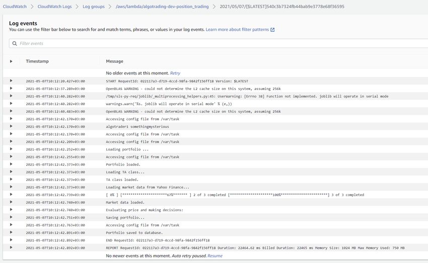
34FIGURE 11. A script for testing the performance of ML model over historical data
As can be seen from the activity logs, this model does not perform very well. Some close-up
observation helps with detecting a few factors which might have contributed to such low
performance:
- The dataset in this scenario was a time-series, which means there was a correlation
between the data points and their time index. However, the Random Forest classifier
treated each datapoint equally regardless of its chronological order, which means it missed
out on one of the most important features of the dataset, leading to a worse performance
classifying the price movement.
35- The model was quite sensitive to changes: if the price moved only as little as 4%, it
considered that an indicator to action. Therefore, even if there was a slight hiccup before
a big jump in price, the model took it as an invocation to sell all the stocks owned, which
means the opportunity was missed. Therefore, more experiment is needed in order to find
the appropriate threshold as to how much price change is considered.
- The model was also quite reactive: it acted upon the price of only the next two days, which
means it did not consider a bigger picture under circumstances such as the one described
above. To tackle this problem, a more sophisticated strategy and evaluation system should
be devised.
Grid search optimization
This is a method aiming to optimize the performance of Machine Learning models. What happens
under the hood is that given a matrix of all necessary hyperparameters, which can be understood
as the settings for a Machine Learning models such as how many loops it learns, the grid search
optimizer computes all the possible combinations of the given values, then with each of them it
constructs a model, trains and evaluates it. This way, the optimizer can find the best combination
of configurations based on the selected evaluation metrics.
In this case, because the model being used was a multiclass Random Forest classifier, the
parameter grid contained parameters such as the number of child trees and the criterion as to how
a node is split. gini and entropy are two only choices provided by the sklearn so both of them were
included here (figure 12). However, readers should consult the documentation of sklearn for more
descriptive information as to how each of them works under the hood.
Figure 12. Random Forest classifier optimization using the Grid search method
36You can also read