Dglke Documentation Release 0.1.0 - dgl-team
←
→
Page content transcription
If your browser does not render page correctly, please read the page content below

dglke Documentation
 Release 0.1.0

 dgl-team

 Feb 11, 2022
Contents

1 Performance and Scalability 3

2 Get started with DGL-KE! 5
 2.1 Installation Guide . . . . . . . . . . . . . . . . . . . . . . . . . . . . . . . . . . . . . . . . . . . . 5
 2.2 Introduction to Knowledge Graph Embedding . . . . . . . . . . . . . . . . . . . . . . . . . . . . . 6
 2.3 DGL-KE Command Lines . . . . . . . . . . . . . . . . . . . . . . . . . . . . . . . . . . . . . . . . 20
 2.4 Train User-Defined Knowledage Graphs . . . . . . . . . . . . . . . . . . . . . . . . . . . . . . . . 45
 2.5 Benchmarks on Built-in Knowledage Graphs . . . . . . . . . . . . . . . . . . . . . . . . . . . . . . 46
 2.6 Profile DGL-KE . . . . . . . . . . . . . . . . . . . . . . . . . . . . . . . . . . . . . . . . . . . . . 49

 i

ii

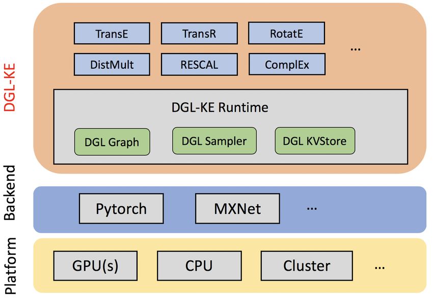
dglke Documentation, Release 0.1.0

Knowledge graphs (KGs) are data structures that store information about different entities (nodes) and their relations
(edges). A common approach of using KGs in various machine learning tasks is to compute knowledge graph embed-
dings. DGL-KE is a high performance, easy-to-use, and scalable package for learning large-scale knowledge graph
embeddings. The package is implemented on the top of Deep Graph Library (DGL) and developers can run DGL-KE
on CPU machine, GPU machine, as well as clusters with a set of popular models, including TransE, TransR, RESCAL,
DistMult, ComplEx, and RotatE.

Contents 1

dglke Documentation, Release 0.1.0

2 Contents

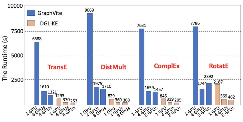
CHAPTER 1

 Performance and Scalability

DGL-KE is designed for learning at scale. It introduces various novel optimizations that accelerate training on knowl-
edge graphs with millions of nodes and billions of edges. Our benchmark on knowledge graphs consisting of over
86M nodes and 338M edges shows that DGL-KE can compute embeddings in 100 minutes on an EC2 instance with 8
GPUs and 30 minutes on an EC2 cluster with 4 machines (48 cores/machine). These results represent a 2×5× speedup
over the best competing approaches.
DGL-KE vs Graphvite

DGL-KE vs Pytorch-Biggraph

 3

dglke Documentation, Release 0.1.0

4 Chapter 1. Performance and Scalability
CHAPTER 2

 Get started with DGL-KE!

2.1 Installation Guide

This topic explains how to install DGL-KE. We recommend installing DGL-KE by using pip and from the source.

2.1.1 System requirements

DGL-KE works with the following operating systems:
 • Ubuntu 16.04 or higher version
 • macOS x
DGL-KE requires Python version 3.5 or later. Python 3.4 or earlier is not tested. Python 2 support is coming.
DGL-KE supports multiple tensor libraries as backends, e.g., PyTorch and MXNet. For requirements on backends and
how to select one, see Working with different backends. As a demo, we install Pytorch using pip:

sudo pip3 install torch

2.1.2 Install DGL

DGL-KE is implemented on the top of DGL (0.4.3 version). You can install DGL using pip:

sudo pip3 install dgl==0.4.3

2.1.3 Install DGL-KE

After installing DGL, you can install DGL-KE. The fastest way to install DGL-KE is by using pip:

 5
dglke Documentation, Release 0.1.0

sudo pip3 install dglke

or you can install DGL-KE from source:

git clone https://github.com/awslabs/dgl-ke.git
cd dgl-ke/python
sudo python3 setup.py install

2.1.4 Have a Quick Test

Once you install DGL-KE successfully, you can test it by the following command:

# create a new workspace
mkdir my_task && cd my_task
# Train transE model on FB15k dataset
DGLBACKEND=pytorch dglke_train --model_name TransE_l2 --dataset FB15k --batch_size
 ˓→1000 \

--neg_sample_size 200 --hidden_dim 400 --gamma 19.9 --lr 0.25 --max_step 500 --log_
 ˓→interval 100 \

--batch_size_eval 16 -adv --regularization_coef 1.00E-09 --test --num_thread 1 --num_
 ˓→proc 8

This command will download the FB15k dataset, train the transE model on that, and save the trained embeddings
into the file. You could see the following output at the end:

-------------- Test result --------------
Test average MRR : 0.47221913961451095
Test average MR : 58.68289854581774
Test average HITS@1 : 0.2784276548560207
Test average HITS@3 : 0.6244265375564998
Test average HITS@10 : 0.7726295474936941
-----------------------------------------

2.2 Introduction to Knowledge Graph Embedding

Knowledge Graphs (KGs) have emerged as an effective way to integrate disparate data sources and model underlying
relationships for applications such as search. At Amazon, we use KGs to represent the hierarchical relationships
among products; the relationships between creators and content on Amazon Music and Prime Video; and information
for Alexa’s question-answering service. Information extracted from KGs in the form of embeddings is used to improve
search, recommend products, and infer missing information.

2.2.1 What is a graph

A graph is a structure used to represent things and their relations. It is made of two sets - the set of nodes (also called
vertices) and the set of edges (also called arcs). Each edge itself connects a pair of nodes indicating that there is a
relation between them. This relation can either be undirected, e.g., capturing symmetric relations between nodes, or
directed, capturing asymmetric relations. For example, if a graph is used to model the friendship relations of people in
a social network, then the edges will be undirected as they are used to indicate that two people are friends; however,
if the graph is used to model how people follow each other on Twitter, the edges will be directed. Depending on the
edges’ directionality, a graph can be directed or undirected.

6 Chapter 2. Get started with DGL-KE!
dglke Documentation, Release 0.1.0

Graphs can be either homogeneous or heterogeneous. In a homogeneous graph, all the nodes represent instances of the
same type and all the edges represent relations of the same type. For instance, a social network is a graph consisting
of people and their connections, all representing the same entity type. In contrast, in a heterogeneous graph, the nodes
and edges can be of different types. For instance, the graph for encoding the information in a marketplace will have
buyer, seller, and product nodes that are connected via wants-to-buy, has-bought, is-customer-of, and is-selling edges.
Finally, another class of graphs that is especially important for knowledge graphs are multigraphs. These are graphs
that can have multiple (directed) edges between the same pair of nodes and can also contain loops. These multiple
edges are typically of different types and as such most multigraphs are heterogeneous. Note that graphs that do not
allow these multiple edges and self-loops are called simple graphs.

2.2.2 What is a Knowledge Graph

In the earlier marketplace graph example, the labels assigned to the different node types (buyer, seller, product) and the
different relation types (wants-to-buy, has-bought, is-customer-of, is-selling) convey precise information (often called
semantics) about what the nodes and relations represent for that particular domain. Once this graph is populated, it
will encode the knowledge that we have about that marketplace as it relates to types of nodes and relations included.
Such a graph is an example of a knowledge graph.
A knowledge graph (KG) is a directed heterogeneous multigraph whose node and relation types have domain-specific
semantics. KGs allow us to encode the knowledge into a form that is human interpretable and amenable to automated
analysis and inference. KGs are becoming a popular approach to represent diverse types of information in the form of
different types of entities connected via different types of relations.
When working with KGs, we adopt a different terminology than the traditional vertices and edges used in graphs.
The vertices of the knowledge graph are often called entities and the directed edges are often called triplets and are
represented as a (h, r, t) tuple, where h is the head entity, t is the tail entity, and r is the relation associating the head with
the tail entities. Note that the term relation here refers to the type of the relation (e.g., one of wants-to-buy, has-bought,
is-customer-of, and is-selling).
Let us examine a directed multigraph in an example, which includes a cast of characters and the world in which they
live.
Scenario:
Mary and Tom are siblings and they both are are vegetarians, who like potatoes and cheese. Mary and Tom both
work at Amazon. Joe is a bloke who is a colleague of Tom. To make the matter complicated, Joe loves Mary, but we
do not know if the feeling is reciprocated.
Joe is from Quebec and is proud of his native dish of Poutine, which is composed of potato, cheese, and gravy. We
also know that gravy contains meat in some form.
Joe is excited to invite Tom for dinner and has sneakily included his sibling, Mary, in the invitation. His plans are
doomed from get go as he is planning to serve the vegetarian siblings his favourite Quebecois dish, Poutine.
Oh! by the way, a piece of geography trivia: Quebec is located in a province of the same name which in turn is located
in Canada.
There are several relationships in this scenario that are not explicitly mentioned but we can simply infer from what we
are given:
 • Mary is a colleague of Tom.
 • Tom is a colleague of Mary.
 • Mary is Tom’s sister.
 • Tom is Mary’s brother.
 • Poutine has meat.

2.2. Introduction to Knowledge Graph Embedding 7
dglke Documentation, Release 0.1.0

 • Poutine is not a vegetarian dish.
 • Mary and Tom would not eat Poutine.
 • Poutine is a Canadian dish.
 • Joe is Canadian.
 • Amazon is a workplace for Mary, Tom, and Joe.
There are also some interesting negative conclusions that seem intuitive to us, but not to the machine: - Potato does not
like Mary. - Canada is not from Joe. - Canada is not located in Quebec. - . . . What we have examined is a knowledge
graph, a set of nodes with different types of relations: - 1-to-1: Mary is a sibling of Tom. - 1-to-N: Amazon is a
workplace for Mary, Tom, and Joe. - N-to-1: Joe, Tom, and Mary work at Amazon. - N-to-N: Joe, Mary, and Tom are
colleagues.
There are other categorization perspectives on the relationships as well: - Symmetric: Joe is a colleague of Tom entails
Tom is also a colleague of Joe. - Antisymmetric: Quebec is located in Canada entails that Canada cannot be located
in Quebec.
Figure 1 visualizes a knowledge-base that describes World of Mary. For more information on how to use the examples,
please refer to the code that draws the examples.

2.2.3 What is the task of Knowledge Graph Embedding?

Knowledge graph embedding is the task of completing the knowledge graphs by probabilistically inferring the missing
arcs from the existing graph structure. KGE differs from ordinary relation inference as the information in a knowledge
graph is multi-relational and more complex to model and computationally expensive. For this rest of this blog, we
examine fundamentals of KGE.

8 Chapter 2. Get started with DGL-KE!
dglke Documentation, Release 0.1.0

2.2.4 Common connectivity patterns:

Different connectivity or relational pattern are commonly observed in KGs. A Knowledge Graph Embedding model
intends to predict missing connections that are often one of the types below.
 • symmetric
 – Definition: A relation is symmetric if ∀ , : ( , , ) =⇒ ( , , )
 – Example: x=Mary and y=Tom and r="is a sibling of";
 ( , , ) = Mary is a sibling of Tom =⇒ ( , , ) = Tom is a sibling of Mary
 • antisymmetric
 – Definition: A relation r is antisymmetric if ∀ , : ( , , ) =⇒ ¬( , , )
 – Example: x=Quebec and y=Canada and r="is located in";
 ( , , ) = Quebec is located in Canada =⇒ ( , ¬ , ) = Canada is not located in Quebec
 • inversion
 – Definition: A relation 1 is inverse to relation 2 if ∀ , : 2 ( , ) =⇒ 1 ( , ).
 – Example: = , = , 1 = "is a sister of” 2 = "is a brother of"
 ( , 1 , ) = Mary is a sister of Tom =⇒ ( , 2 , ) = Tom is a brother of Mary
 • composition
 – Definition: relation 1 is composed of relation 2 and relation 3 if ∀ , , : ( , 2 , )∧( , 3 , ) =⇒
 ( , 1 , )
 – Example: x=Tom, y=Quebec, z=Canada, 2 = "is born in", 3 = "is located in", 1 = "is from"
 ( , 2 , ) = Tom is born in Quebec ∧ ( , 3 , ) = Quebec is located in Canada
 =⇒ ( , 1 , ) = Tom is from Canada
ref: RotateE[2]

2.2.5 Score Function

There are different flavours of KGE that have been developed over the course of the past few years. What most of
them have in common is a score function. The score function measures how distant two nodes relative to its relation
type. As we are setting the stage to introduce the reader to DGL-KE, an open source knowledge graph embedding
library, we limit the scope only to those methods that are implemented by DGL-KE and are listed in Figure 2.
Figure2: A list of score functions for KE papers implemented by DGL-KE

2.2. Introduction to Knowledge Graph Embedding 9
dglke Documentation, Release 0.1.0

2.2.6 A short explanation of the score functions

Knowledge graphs that are beyond toy examples are always large, high dimensional, and sparse. High dimensionality
and sparsity result from the amount of information that the KG holds that can be represented with 1-hot or n-hot
vectors. The fact that most of the items have no relationship with one another is another major contributor to sparsity
of KG representations. We, therefore, desire to project the sparse and high dimensional graph representation vector
space into a lower dimensional dense space. This is similar to the process used to generate word embeddings and
reduce dimensions in recommender systems based on matrix factorization models. I will provide a detailed account of
all the methods in a different post, but here I will shortly explain how projections differ in each paper, what the score
functions do, and what consequences the choices have for relationship inference and computational complexity.

TransE:

TransE is a representative translational distance model that represents entities and relations as vectors in the same
semantic space of dimension R, where is the dimension of the target space with reduced dimension. A fact in
the source space is represented as a triplet (ℎ, , ) where ℎ is short for head, is for relation, and is for tail.
The relationship is interpreted as a translation vector so that the embedded entities are connected by relation have
a short distance. [3, 4] In terms of vector computation it could mean adding a head to a relation should approx-
imate to the relation’s tail, or ℎ + ≈ . For example if ℎ1 = (” ”), ℎ2 = (” ”), 1 =
 (” ”), 2 = (” ”), and finally = ” ”, then ℎ1 + and ℎ2 + should approximate
 1 and 2 respectively. TransE performs linear transformation and the scoring function is negative distance between
ℎ + and , or = −‖ℎ + − ‖ 12
Figure 3: TransE

10 Chapter 2. Get started with DGL-KE!
dglke Documentation, Release 0.1.0

TransR

TransE cannot cover a relationship that is not 1-to-1 as it learns only one aspect of similarity. TransR addresses this
issue with separating relationship space from entity space where ℎ, ∈ R and ∈ R . The semantic spaces do not
need to be of the same dimension. In the multi-relationship modeling we learn a projection matrix ∈ R × for
each relationship that can project an entity to different relationship semantic spaces. Each of these spaces capture a
different aspect of an entity that is related to a distinct relationship. In this case a head node ℎ and a tail node in
relation to relationship is projected into the relationship space using the learned projection matrix as ℎ = ℎ
and = respectively. Figure 5 illustrates this projection.
Let us explore this using an example. Mary and Tom are siblings and colleagues. They both are vegetarians. Joe also
works for Amazon and is a colleague of Mary and Tom. TransE might end up learning very similar embeddings for
Mary, Tom, and Joe because they are colleagues but cannot recognize the (not) sibling relationship. Using TransR, we
learn projection matrices: , and that perform better at learning relationship like (not)sibling.
The score function in TransR is similar to the one used in TransE and measures euclidean distance between ℎ + and
 , but the distance measure is per relationship space. More formally: = ‖ℎ + − ‖22
Figure 4: TransR projecting different aspects of an entity to a relationship space.

Another advantage of TransR over TransE is its ability to extract compositional rules. Ability to extract rules has two
major benefits. It offers richer information and has a smaller memory space as we can infer some rules from others.

Drawbacks

The benefits from more expressive projections in TransR adds to the complexity of the model and a higher rate of data
transfer, which has adversely affected distributed training. TransE requires ( ) parameters per relation, where is
the dimension of semantic space in TransE and includes both entities and relationships. As TransR projects entities
to a relationship space of dimension , it will require ( ) parameters per relation. Depending on the size of k, this
could potentially increase the number of parameters drastically. In exploring DGL-KE, we will examine benefits of
DGL-KE in making computation of knowledge embedding significantly more efficient.
ref: TransR[5], 7
TransE and its variants such as TransR are generally called translational distance models as they translate the entities,
relationships and measure distance in the target semantic spaces. A second category of KE models is called semantic
matching that includes models such as RESCAL, DistMult, and ComplEx.These models make use of a similarity-based
scoring function.
The first of semantic matching models we explore is RESCAL.

2.2. Introduction to Knowledge Graph Embedding 11
dglke Documentation, Release 0.1.0

RESCAL

RESCAL is a bilinear model that captures latent semantics of a knowledge graph through associate entities with
vectors and represents each relation as a matrix that models pairwise interaction between entities.
Multiple relations of any order can be represented as tensors. In fact − tensors are by definition
representations of multi-dimensional vector spaces. RESCAL, therefore, proposes to capture entities and relationships
as multidimensional tensors as illustrated in figure 5.
RESCAL uses semantic web’s RDF formation where relationships are modeled as ( , , ). Ten-
sor contains such relationships as between th and th entities through th relation. Value of is determined
as:
 {︃
 1 if ( , , ) holds
 =
 0 if ( , , ) does not hold

Figure 5: RESCAL captures entities and their relations as multi-dimensional tensor

As entity relationship tensors tend to be sparse, the authors of RESCAL, propose a dyadic decomposition to capture
the inherent structure of the relations in the form of a latent vector representation of the entities and an asymmetric
square matrix that captures the relationships. More formally each slice of is decomposed as a rank− factorization:

 ≈ A⊤ , for = 1, . . . ,

where A is an × matrix of latent-component representation of entities and asymmetrical × square matrix

12 Chapter 2. Get started with DGL-KE!
dglke Documentation, Release 0.1.0
that models interaction for ℎ predicate component in . To make sense of it all, let’s take a look at an example:
= {Mary :0, Tom :1, Joe :2} (2.1)
ℎ = {sibling, colleague} (2.2)
=0 : Mary and Tom are siblings but Joe is not their sibling. (2.3)
=1 : Mary,Tom, and Joe are colleagues (2.4)
⎡ ⎤
relationship matrices will model: ‖ = ⎣ ⎦ (2.5)
⎡ ⎤
0 1 0
0: = ⎣0 0 1⎦ (2.6)
0 0 0
⎡ ⎤
0 1 1
1: = ⎣1 0 1⎦ (2.7)
1 1 0
Note that even in such a small knowledge graph where two of the three entities have even a symmetrical relationship,
matrices are sparse and asymmetrical. Obviously colleague relationship in this example is not representative of
a real world problem. Even though such relationships can be created, they contain no information as probability of
occurring is high. For instance if we are creating a knowledge graph for for registered members of a website is a
specific country, we do not model relations like “is countryman of” as it contains little information and has very low
entropy.
Next step in RESCAL is decomposing matrices using a rank_k decomposition as illustrated in figure 6.
Figure 6: Each of the slices of martix is factorized to its k-rank components in form of a × entity-latent
component and an asymmetric × that specifies interactions of entity-latent components per relation.
and are computed through solving an optimization problem that is correlated to minimizing the distance between
and A⊤ .
Now that the structural decomposition of entities and their relationships are modeled, we need to create a score function
that can predict existence of relationship for those entities we lack their mutual connection information.
The score function (ℎ, ) for ℎ, ∈ R , where ℎ and are representations of head and tail entities, captures pairwise
interactions between entities in ℎ and through relationship matrix that is the collection of all individual
matrices and is of dimension × .
−1 ∑︁
∑︁ −1
(ℎ, ) = h⊤ = [ ] .[ℎ] .[ ]
=0 =0
Figure 7 illustrates computation of the the score for RESCAL method.
Figure 7: RESCAL
2.2. Introduction to Knowledge Graph Embedding 13dglke Documentation, Release 0.1.0 Score function requires ( 2 ) parameters per relation. Ref: 6,7 DistMult If we want to speed up the computation of RESCAL and limit the relationships only to symmetric relations, then we can take advantage of the proposal put forth by DistMult[8], which simplifies RESCAL by restricting from a general asymmetric × matrix to a diagonal square matrix, thus reducing the number of parameters per relation to ( ). DistMulti introduces vector embedding ∈ ℛ . is computed as: −1 ∑︁ (ℎ, ) = h⊤ ( ) = [ ] .[ℎ] .[ ] =0 Figure 8 illustrates how DistMulti computes the score by capturing the pairwise interaction only along the same dimensions of components of h and t. Figure 8: DistMulti 14 Chapter 2. Get started with DGL-KE!
dglke Documentation, Release 0.1.0

A basic refresher on linear algebra

 ⎡ ⎤ ⎡ ⎤
 11 12 ... 1 11 12 ... 1
 ⎢ 21 22 ... 2 ⎥ ⎢ 21 22 ... 2 ⎥
 = [ ] × =⎢ . and = [ ] × = ⎢ .
 ⎢ ⎥ ⎢ ⎥
 .. .. .. ..
 ⎣ .. ⎣ ..
 ⎥ ⎥
 . . ... ⎦ . . . . .⎦
 1 2 . . . × 1 2 ... ×

 ∑︁
 ℎ = [ ] × ℎ ℎ = ℎ :
 =1
 ⎡ ⎤
 11 11 + · · · + 1 1 11 12 + · · · + 1 2 ... 11 1 + · · · + 1
 ⎢ 21 11 + · · · + 2 1 21 12 + · · · + 2 2 ... 21 1 + · · · + 2 ⎥
 × = ⎢
 ⎢ ⎥
 .. .. .. ⎥
 ⎣ . . . ... ⎦
 1 11 + · · · + 1 1 12 + · · · + 2 ... 1 1 + · · · + ×

We know that a diagonal matrix is a matrix in which all non diagonal elements, ( ̸= ), are zero. This reduces
complexity of matrix multiplication as for diagonal matrix multiplication for diagonal matrices × and × ,
 = = [ ] × where
 {︃
 0 for ̸=
 =
 for =

This is basically multiplying to numbers and to get the value for the corresponding diagonal element on .
This complexity reduction is the reason that whenever possible we would like to reduce matrices to diagonal matrices.

ComplEx

In order to model a KG effectively, models need to be able to identify most common relationship patters as laid out
earlier in this blog. relations can be reflexive/irreflexive, symmetric/antisymmetric, and transitive/intransitive. We
have also seen two classes of semantic matching models, RESCAL and DistMulti. RESCAL is expressive but has an
exponential complexity, while DistMulti has linear complexity but is limited to symmetric relations.
An ideal model needs to keep linear complexity while being able to capture antisymmetric relations. Let us go back
to what is good at DistMulti. It is using a rank-decomposition based on a diagonal matrix. We know that dot product
of embedding scale well and handles symmetry, reflexity, and irreflexivity effectively. Matrix factorization (MF)
methods have been very successful in recommender systems. MF works based on factorizing a relation matrix to
dot product of lower dimensional matrices UV⊤ where UV ∈ R × . The underlying assumption here is that the
same entity would be taken to be different depending on whether it appears as a subject or an object in a relationship.
For instance “Quebec” in “Quebec is located in Canada” and “Joe is from Quebec” appears as subject and object
respectively. In many link prediction tasks the same entity can assume both roles as we perform graph embedding
through adjacency matrix computation. Dealing with antisymmetric relationships, consequently, has resulted in an
explosion of parameters and increased complexity and memory requirements.
The goal ComplEx is set to achieve is performing embedding while reducing the number of required parameters, to
scale well, and to capture antisymmetric relations. One essential strategy is to compute a joint representation for the
entities regardless of their role as subject or object and perform dot product on those embeddings.
Such embeddings cannot be achieved in the real vector spaces, so the ComplEx authors propose complex embedding.
 √
But first a quick reminder about complex vectors. #### Complex Vector Space 1 is the unit for real numbers, = −1
is the imaginary unit of complex numbers. Each complex number has two parts, a real and an imaginary part and is
represented as = + ∈ C. As expected, the complex plane has a horizontal and a vertical axis. Real numbers

2.2. Introduction to Knowledge Graph Embedding 15
dglke Documentation, Release 0.1.0 are placed on the horizontal axis and the vertical axis represents the imaginary part of a number. This is done in much the same way as in and are represented on Cartesian plane. An n-dimensional complex vector ∈ C is a vector whose elements ∈ C are complex numbers. Example: ⎡ ⎤ [︂ ]︂ 2 + 3 2 + 3 1 = and 2 = ⎣1 + 5 ⎦ are in C2 and C3 respectively. 1 + 5 3 R ⊂ C and R ⊂ C . Basically a real number is a complex number whose imaginary part has a coefficient of zero. modulus of a complex number is √a complex number as is given by = + , modulus is analogous to size in vector space and is given by | |= 2 + 2 Complex Conjugate The conjugate of complex number = + is denoted by ¯ and is given by ¯ = − . Example: ⎡ ⎤ [︂ ]︂ 2 − 3 2 − 3 ¯1 = and ¯2 = ⎣1 − 5 ⎦ are in C2 and C3 respectively. 1 − 5 3 Conjugate Transpose The conjugate transpose of a complex matrix , is denoted as * and is given by * = ¯⊤ where elements of ¯ are complex conjugates of . Example: 1* = 2 − 3 1 − 5 and 2* = 2 − 3 3 are in C2 and C3 respectively. [︀ ]︀ [︀ ]︀ 1 − 5 Complex dot product. aka Hermitian inner product if u and c are complex vectors, then their inner product is defined as ⟨u, v⟩ = u* v. Example: [︂ ]︂ [︂ ]︂ 2 + 3 1+ = and = are in C2 and C3 respectively. 1 + 5 2 + 2 then * = 2 − 3 1 − 5 and [︀ ]︀ [︂ ]︂ ]︀ 1 + ⟨ , ⟩ = * = 2 − 3 [︀ 1 − 5 = (2 − 3 )(1 + ) + (1 − 5 )(2 + 2 ) = [4 − 13 ] 2 + 2 Definition: A complex matrix us unitary when −1 = * [︂ ]︂ 1+ 1− Example: = 12 1− 1+ Theorem: An × complex matrix is unitary ⇐⇒ its rows or columns form an orthanormal set in Definition: A square matrix is Hermitian when = * [︂ ]︂ 1 1 + 2 Example: = 1 + 2 +1 Theorem: Matrix is Hermitian ⇐⇒ : 1. ∈ R 2. is complex conjugate of Theorem: If is a Hermirian matrix, then its eigenvalues are real numbers. Theorem: Hermitian matrices are unitarity diagonizable. Definitions: A squared matrix A is unitarily diagonizable when there exists a unitary matrix such that −1 . Diagonizability can be extended to a larger class of matrices, called normal matrices. 16 Chapter 2. Get started with DGL-KE!
dglke Documentation, Release 0.1.0

Definition: A square complex matrix A is called normal when it commutes with its conjugate transpose. * = * .
Theorem: A complex matrix is normal ⇐⇒ is diagonizable.
This theorem plays a crucial role in ComplEx paper.
ref: https://www.cengage.com/resource_uploads/downloads/1133110878_339554.pdf

Eigen decomposition for entity embedding

The matrix decomposition methods have a long history in machine learning. Using embeddings based decomposition
in the form of = −1 for square symmetric matrices can be represented as eigen decomposition = Λ −1
where is orthogonal (|= −1 = ⊤ ) and Λ = ( ) and is an eigenvector of .
As ComplEx targets to learn antisymmetric relations, and eigen decomposition for asymmetric matrices does not
exist in real space, the authors extend the embedding representation to complex numbers, where they can factorize
complex matrices and benefit from efficient scaling and distribution of matrix multiplication while being able to capture
antisymmetric relations. This asymmetry is resulted from the fact that dot product of complex matrices involves
conjugate transpose.
We are not done yet. Do you remember in RESCAL the number of parameters was ( 2 ) and DistMulti reduce that
to a linear relation of ( ) by limiting matrix to be diagonal?. Here even with complex eigenvectors ∈ × ,
inversion of in = * explodes the number of parameters. As a result we need to find a solutions in which
W is a diagonal matrix, and = * , and is asymmetric, so that we 1) computation is minimized, 2) there is no
need to compute inverse of , and 3) antisymmetric relations can be captures. We have already seen the solution
in the complex vector space section. The paper does construct the decomposition in a normal space, a vector space
composed of complex normal vectors.

The Score Function

A relation between two entities can be modeled as a sign function, meaning that if there is a relation between a subject
and an object, then the score is 1, otherwise it is -1. More formally, ∈ {−1, 1}. The probability of a relation
between two edntities to exist is then given by sigmoid function: ( = 1) = ( ).
This probability score requires to be real, while * includes both real and imaginary components. We can
simply project the decomposition to the real space so that = ( * ). the score function of ComlEx, therefore
is given by:
 −1
 ∑︁
 (ℎ, ) = (ℎ⊤ ( ) ¯) = ( [ ] .[ℎ] .[ ¯] )
 =0

and since there are no nested loops, the number of parameters is linear and is given by ( ).

RotateE

Let us reexamine translational distance models with the ones in latest publications on relational embedding models
(RotateE). Inspired by TransE, RotateE veers into complex vector space and is motivated by Euler’s identity, defines
relations as rotation from head to tail.

Euler’s Formula

 can be computed using the infinite series below:
 2 3 4 5 6 7 8
 = 1 + + + + + + + + + ...
 1! 2! 3! 4! 5! 6! 7! 8!

2.2. Introduction to Knowledge Graph Embedding 17
dglke Documentation, Release 0.1.0
replacing with entails:
2 3 2 5 6 7 8
( ) = 1 + − − + + − − + + ...
1! 2! 3! 4! 5! 6! 3! 8!
Computing to a sequence of powers and replacing the values in :math:‘e^{ix} ‘ the the results in:
2 = −1, 3 = 2 = − , 4 = 3 = −12 = 1, 5 = 4 = , 6 = 5 = 2 = −1, . . .
2 2 3 3 4 4 5 5 6 6
( ) = 1 + + + + + + + ...
1! 2! 3! 4! 5! 6!
rearranging the series and factoring in terms that include it:
2 4 6 8 3 5 7
(︂ )︂
1− + − + + − + − (1)
2! 4! 6! 8! 1! 3! 5! 7!
and representation as series are given by:
3 5 7
( ) = − + − + ...
1! 3! 5! 7!
2 4 6 8
( ) = 1 − + − + + ...
2! 4! 6! 8!
Finally replacing terms in equation (1) with and , we have:
= ( ) + ( ) (2)
Equation 2 is called Euler’s formula and has interesting consequences in a way that we can represent complex numbers
as rotation on the unit circle.
Modeling Relations as Rotation
Given a triplet (ℎ, , ), = ℎ ∘ , where ℎ, , and ∈ C are the embeddings. modulus | |= 1(as we are in the unit
circle thanks to Euler’s formula), and ∘ is the element-wise product. We, therefore, for each dimension expect to have:
= ℎ , where ℎ , , ∈ C, | |= 1.
Restricting | |= 1 will be of form , . Intuitively corresponds to a counterclockwise rotation by , based
on Eurler’s formula.
0
Under these conditions,: - is symmetric ⇐⇒ ∀ ∈ (0, ] : = = ±1. - 1 and 2 are inverse ⇐⇒ 2 = ¯1
(embeddings of relations are complex conjugates) - 3 = 3 is a combination of 1 = 1 and 2 = 2 ⇐⇒ 3 =
1 ∘ 2 .( . ) 3 = 1 + 2 or a rotation is a combination of two smaller rotations sum of whose angles is the angle of
the third relation.
Figure 9: RotateE vs. TransE
18 Chapter 2. Get started with DGL-KE!dglke Documentation, Release 0.1.0 Score Function score function of RotateE measures the angular distance between head and tail elements and is defined as: (ℎ, ) = ‖ℎ ∘ − ‖ 2.2.7 Training KE 2.2.8 Negative Sampling Generally to train a KE, all the models we have investigated apply a variation of negative sampling by corrupting triplets (ℎ, , ). They corrupt either ℎ, or by by sampling from set of head or tail entities for heads and tails respectively. The corrupted triples can be of wither forms (ℎ′ , , ) or (ℎ, , ′ ), where ℎ′ and ′ are the negative samples. 2.2.9 Loss functions Most commonly logistic loss and pairwise ranking loss are employed. The logistic loss returns -1 for negative samples and +1 for the positive samples. So if D+ and D− are negative and positive data, = ±1 is the label for positive and negative triplets and (figure 2) is the ranking function, then the logistic loss is computed as: ∑︁ (1 + − × (ℎ, , ) ) (ℎ, , )∈D+ ∪D− The second commonly use loss function is margin based pairwise ranking loss, which minimizes the rank for positive triplets((ℎ, , ) does hold). The lower the rank, the higher the probability. Ranking loss is give by: ∑︁ ∑︁ (0, − (ℎ, , ) + (ℎ′ , ′ , ′ )). (ℎ, , )∈D+ (ℎ, , )∈D− Method Ent. Embed- Rel. Emebed- Score Function Com- symm Anti Inv Comp ding ding plexity TransE ℎ, ∈ R ∈ R −‖ℎ + − ‖ ( ) − X X − TransR ℎ, ∈ R ∈ R , ∈ −‖ ℎ + − ( 2 ) − X X X R × ‖22 RESCAL ℎ, ∈ R ∈ R × ℎ⊤ ( 2 ) X − X X Dist- ℎ, ∈ R ∈ R ℎ⊤ ( ) ( ) X − − − Multi Com- ℎ, ∈ C ∈ C ℎ⊤ ( ( ) ) ( ) X X X − plEx RotateE ℎ, ∈ C ∈ C ‖ℎ ∘ − ‖ ( ) X X X X 2.2.10 References 1. http://semantic-web-journal.net/system/files/swj1167.pdf 2. Zhiqing Sun, Zhi-Hong Deng, Jian-Yun Nie, and Jian Tang. RotatE: Knowledge graph embedding by relational rotation in complex space. CoRR, abs/1902.10197, 2019. 3. Knowledge Graph Embedding: A Survey of Approaches and Applications Quan Wang, Zhendong Mao, Bin Wang, and Li Guo. DOI 10.1109/TKDE.2017.2754499, IEEE Transactions on Knowledge and Data Engineer- ing 2.2. Introduction to Knowledge Graph Embedding 19
dglke Documentation, Release 0.1.0

 4. transE: Antoine Bordes, Nicolas Usunier, Alberto Garcia-Duran, JasonWeston, and Oksana Yakhnenko. Trans-
 lating embeddings for modeling multi-relational data. In Advances in Neural Information Processing Systems
 26. 2013. 5.TransR: Yankai Lin, Zhiyuan Liu, Maosong Sun, Yang Liu, and Xuan Zhu. Learning entity and
 relation embeddings for knowledge graph completion. In Proceedings of the Twenty-Ninth AAAI Conference
 on Artificial Intelligence, 2015.
 5. RESCAL: Maximilian Nickel, Volker Tresp, and Hans-Peter Kriegel. A three-way model for collective learning
 on multi-relational data. In Proceedings of the 28th International Conference on International Conference on
 Machine Learning, ICML’11, 2011.
 6. Survey paper: Q. Wang, Z. Mao, B. Wang and L. Guo, “Knowledge Graph Embedding: A Survey of Approaches
 and Applications,” in IEEE Transactions on Knowledge and Data Engineering, vol. 29, no. 12, pp. 2724-2743,
 1 Dec. 2017.
 7. DistMult: Bishan Yang, Scott Wen-tau Yih, Xiaodong He, Jianfeng Gao, and Li Deng. Embedding entities
 and relations for learning and inference in knowledge bases. In Proceedings of the International Conference on
 Learning Representations (ICLR) 2015, May 2015.
 8. ComplEx: Théo Trouillon, Johannes Welbl, Sebastian Riedel, Éric Gaussier, and Guillaume Bouchard. Com-
 plex embeddings for simple link prediction. CoRR, abs/1606.06357, 2016.
 9. Zhiqing Sun, Zhi-Hong Deng, Jian-Yun Nie, and Jian Tang. RotatE: Knowledge graph embedding by relational
 rotation in complex space. CoRR, abs/1902.10197, 2019.

2.3 DGL-KE Command Lines

DGL-KE provides a set of command line tools to train knowledge graph embeddings and make prediction with the
embeddings easily.

2.3.1 Format of Input Data

DGL-KE toolkits provide commands for training, evaluation and inference. Different commands require different
kinds of input data, including:
 • Knowledge Graph The knowledge graph used in train, evaluation and inference.
 • Trained Embeddings The embedding generated by dglke_train or dglke_dist_train.
 • Other Data Extra input data that used by inference tools.
A knowledge graph is usually stored in the form of triplets (head, relation, tail). Heads and tails are entities in the
knowledge graph. All of them can be identified with unique IDs. In general, there exists two types of IDs for entities
and relations in DGL-KE:
 • Raw ID The entities and relations can be identified by names, usually in the format of strings.
 • KGE ID They are used during knowledge graph training, evaluation and inference. Both entities and relations
 are identified with integers and should start from 0 and be contiguous.
If the input file of a knowledge graph uses Raw IDs for entities and relations and does not provide a mapping between
Raw IDs and KGE Ids, DGL-KE will generate an ID mapping automatically.
The following table gives the overview of the input data for different toolkits. (Y for necessary and N for no-usage)

20 Chapter 2. Get started with DGL-KE!
dglke Documentation, Release 0.1.0

 DGL-KE Toolkit Knowledge Graph Trained Embeddings Other Data
 Triplets ID Mapping Embeddings
 dglke_train Y Y N N
 dglke_eval Y N Y N
 dglke_partition Y Y N N
 dglke_dist_train Use data generated by dglke_partition
 dglke_predict N Y Y Y
 dglke_emb_sim N Y Y Y

Format of Knowledge Graph Used by DGL-KE

DGL-KE support three kinds of Knowledge Graph Input:
 • Built-in Knowledge Graph Built-in knowledge graphs are preprocessed datasets provided by DGL-KE pack-
 age. There are five built-in datasets: FB15k, FB15k-237, wn18, wn18rr, Freebase.
 • Raw User Defined Knowledge Graph Raw user defined knowledge graph dataset uses the Raw IDs. Necessary
 ID convertion is needed before training a KGE model on the dataset. dglke_train, dglke_eval and
 dglke_partition provides the basic ability to do the ID convertion automatically.
 • KGE User Defined Knowledge Graph KGE user defined knowledge graph dataset already uses KGE IDs. The
 entities and relations in triplets are integers.

Format of Built-in Knowledge Graph

DGL-KE provides five built-in knowledge graphs:

 Dataset #nodes #edges #relations
 FB15k 14,951 592,213 1,345
 FB15k-237 14,541 310,116 237
 wn18 40,943 151,442 18
 wn18rr 40,943 93,003 11
 Freebase 86,054,151 338,586,276 14,824

Each of these built-in datasets contains five files:
 • train.txt: training set, each line contains a triplet [h, r, t]
 • valid.txt: validation set, each line contains a triplet [h, r, t]
 • test.txt: test set, each line contains a triplet [h, r, t]
 • entities.dict: ID mapping of entities
 • relations.dict: ID mapping of relations

Format of Raw User Defined Knowledge Graph

Raw user defined knowledge graph dataset uses the Raw IDs. The knowledge graph can be stored in a single file (only
providing the trainset) or in three files (trainset, validset and testset). Each file stores the triplets of the knowledge
graph. The order of head, relation and tail can be arbitry, e.g. [h, r, t]. A delimiter should be used to seperate them.
The recommended delimiter includes \t, |, , and ;. The ID mapping is automatically generated by DGL-KE toolkits
for raw user defined knowledge graphs.

2.3. DGL-KE Command Lines 21
dglke Documentation, Release 0.1.0

One extra column can be provided to store edge importance score value after hrt. The importance score can be used
in training to highlight the importance of positive edges. The scores should be floats.
Following gives an example of Raw User Defined Knowledge Graph files:
train.txt:

"Beijing","is_capital_of","China"
"Paris","is_capital_of","France"
"London","is_capital_of","UK"
"UK","located_at","Europe"
"China","located_at","Asia"
"Tokyo","is_capital_of","Japan"

valid.txt:

"France","located_at","Europe"

test.txt:

"Japan","located_at","Asia"

Following gives an example of Raw User Defined Knowledge Graph with edge importance score.
train.txt:

"Beijing","is_capital_of","China",2.0
"Paris","is_capital_of","France",1.0

Format of User Defined Knowledge Graph

User Defined Knowledge Graph uses the KGE IDs, which means both the entities and relations have already been
remapped. The entity IDs and relation IDs are both start from 0 and be contiguous. The knowledge graph can be
stored in a single file (only providing the trainset) or in three files (trainset, validset and testset) along with two ID
mapping files (one for entity ID mapping and another for relation ID mapping). The knowledge graph is stored as
triplets in files. The order of head, relation and tail can be arbitry, e.g. [h, r, t]. A delimiter should be used to seperate
them. The recommended delimiter includes \t, |, , and ;. The ID mapping information is stored as pairs in mapping
files with pair[0] as the integer ID and pair[1] as the original raw ID. The dglke_train and dglke_dist_train
will do some integrity check of the IDs according to the mapping files.
One extra column can be provided to store edge importance score value after hrt. The importance score can be used
in training to highlight the importance of positive edges. The scores should be floats.
Following gives an example of User Defined Knowledge Graph files:
train.txt:

0,0,1
2,0,3
4,0,5
5,1,6
1,1,7
8,0,9

valid.txt:

3,1,6

22 Chapter 2. Get started with DGL-KE!
dglke Documentation, Release 0.1.0

test.txt:

9,1,7

Following gives an example of Raw User Defined Knowledge Graph with edge importance score.
train.txt:

0,0,1,2.0
2,0,3,1.0

Following gives an example of entity ID mapping file:
entities.dict:

0,"Beijing"
1,"China"
2,"Paris"
3,"France"
4,"London"
5,"UK"
6,"Europe"
7,"Asia"
8,"Tokyo"
9,"Japan"

Following gives an example of relation ID mapping file:
relations.dict:

0,"is_capital_of"
1,"located_at"

Format of Trained Embeddings

The trained embeddings are generated by dglke_train or dglke_dist_train CMD. The trained embeddings
are stored in npy format. Usually there are two files:
 • Entity embeddings Entity embeddings are stored in a file named in format of
 dataset_name>__entity.npy and can be loaded through numpy.load().
 • Relation embeddings Relation embeddings are stored in a file named in format of
 dataset_name>__relation.npy and can be loaded through numpy.load()

Format of Input Data Used by DGL-KE Inference Tools

Both dglke_predict and dglke_emb_sim require user provied list of inferencing object.

Format of Raw Input Data

Raw Input Data uses the Raw IDs. Thus the input file contains objects in raw IDs and necessary ID mapping file(s)
are required. Each line of the input file contains only one object and it can contains multiple lines. The ID mapping
file store mapping information in pairs with pair[0] as the integer ID and pair[1] as the original raw ID.
Following gives an example of raw input files for dglke_predict:
head.list:

2.3. DGL-KE Command Lines 23
dglke Documentation, Release 0.1.0

"Beijing"
"London"

rel.list:

"is_capital_of"

tail.list:

"China"
"France"
"UK"

entities.dict:

0,"Beijing"
1,"China"
2,"Paris"
3,"France"
4,"London"
5,"UK"
6,"Europe"

relations.dict:

0,"is_capital_of"
1,"located_at"

Format of KGE Input Data

KGE Input Data uses the KGE IDs. Thus the input file contains objects in KGE IDs, i.e., intergers. Each line of the
input file contains only one object and it can contains multiple lines.
Following gives an example of raw input files for dglke_predict:
head.list:

0
4

rel.list:

0

tail.list:

1
3
5

2.3.2 Format of Output

Different DGL-KE command line toolkits has different output data. Basically they have following dependency:
 • dglke_dist_train depends on the output of dglke_partition

24 Chapter 2. Get started with DGL-KE!
dglke Documentation, Release 0.1.0

 • dglke_eval depends on the output (Trained Embeddings) of the training CMD dglke_train or
 dglke_dist_train
 • dglke_predict and dglke_emb_sim depends on the the output (Trained Embeddings) of the training
 CMD dglke_train or dglke_dist_train as well as the ID mapping file.

Output format of dglke_partition

dglke_partition parititions a graph into parts. It generates N partition directories according to the input argu-
ment -k N. For example, when we set -k to 4, it will generate 4 directories: partition_0, partition_1,
partition_2, and partition_3.
The detailed format of each partition_n is used by dglke_dist_train only and is out of the current scope.
Please refer to distributed train section for more details.

Output format of dglke_train and dglke_dist_train

The output of dglke_train and dglke_dist_train are almost the same. Here we explain the output of
dglke_train in this paragraph.
Basically there are four outputs:
 • Traned Embeddings: The saved model. For most of models like TransE, RESCAL, DistMult,
 ComplEx, and RotatE, there will be two files: __entity.npy for entity
 embedding and __relation.npy for relation embedding. There are all
 saved numpy tensor objects. For TransR, there is one additional output for saving the projection
 matrix.
 • config.json: The config file records all the details of the training configurations as well as the loca-
 tions of ID mapping files generated by dgl_train. The fields of the config file are shown below:

 Field Name Explanation
 neg_sample_size int value of param –neg_sample_size
 max_train_step int value of param –max_step
 double_ent bool value of param –double_ent
 rmap_file relation ID mapping file name
 lr float value of param –lr
 neg_adversarial_sampling bool value of param –neg_adversarial_sampling
 gamma float value of param – gamma
 adversarial_temperature float value of param – adversarial_temperature
 batch_size int value of param – batch_size
 regularization_coef float value of param –regularization_coef
 model model name
 dataset dataset name
 emb_size embedding dimention size
 regularization_norm int value of param –regularization_norm
 double_rel bool value of param –double_rel
 emap_file entity ID mapping file name

 • Training Log: The output log printed to stdout. If --test is set. The final test result is also output
 (MR, MRR, Hit@1, Hit@3, Hit@10).
 • ID mapping Files (Optional): The the input data is in format of Raw User Defined Knowledge
 Graph, that is all triplets use the Raw ID space. The training script will do the ID convertion and
 generate two ID mapping files:

2.3. DGL-KE Command Lines 25
dglke Documentation, Release 0.1.0

 – entities.tsv, for entity ID mapping in format of KGE_entity_ID\tRaw_entity_Name,
 for example:
 0\tBeijing
 1\tChina”
 – relations.tsv, for relation ID mapping in format of KGE_relation_ID\tRaw_relation_name,
 for example:
 0\tis_capital_of
 1\tlocated_at

Output format of dglke_eval

There will be only one output of dglke_eval, the testing result including MR, MRR, Hit@1, Hit@3, Hit@10.

Output format of dglke_predict

The output of dglke_predict is a list of top ranked candidate (h, r, t) triplets as well as their prediction scores.
The output is by default written into result.tsv and in the format of ‘src\trel\tdst\tscore’.
The example output is as:

src rel dst score
6 0 15 -2.39380
8 0 14 -2.65297
2 0 14 -2.67331
9 0 18 -2.86985
8 0 20 -2.89651

If the input data of dglke_predict is in Raw IDs, dglke_predict will also convert the output result in Raw
IDs.
The example output is as:: head rel tail score 08847694 _derivationally_related_form 09440400 -7.41088 08847694
 _hyponym 09440400 -8.99562 02537319 _derivationally_related_form 01490112 -9.08666 02537319 _hy-
 ponym 01490112 -9.44877 00083809 _derivationally_related_form 05940414 -9.88155

Output format of dglke_emb_sim

The output of dglke_emb_sim is a list of top ranked candidate (left, right) pairs as well as their embedding similarity
scores. The output is by default written into result.tsv and in the format of ‘left\tright\tscore’.
The example output is as:

left right score
6 15 0.55512
1 12 0.33153
7 20 0.27706
7 19 0.25631
7 13 0.21372

If the input data of dglke_emb_sim is in Raw IDs, dglke_emb_sim will also convert the output result in Raw
IDs.
The example output is as:

26 Chapter 2. Get started with DGL-KE!
dglke Documentation, Release 0.1.0

left right score
_hyponym _hyponym 0.99999
_derivationally_related_form _derivationally_related_form 0.99999
_hyponym _also_see 0.58408
_hyponym _member_of_domain_topic 0.44027
_hyponym _member_of_domain_region 0.30975

2.3.3 Training in a single machine

dglke_train trains KG embeddings on CPUs or GPUs in a single machine and saves the trained node embeddings
and relation embeddings on disks.

Arguments

The command line provides the following arguments:
 • --model_name {TransE, TransE_l1, TransE_l2, TransR, RESCAL, DistMult,
 ComplEx, RotatE, SimplE} The models provided by DGL-KE.
 • --data_path DATA_PATH The path of the directory where DGL-KE loads knowledge graph data.
 • --dataset DATA_SET The name of the knowledge graph stored under data_path. If it is one of the builtin
 knowledge grpahs such as FB15k, FB15k-237, wn18, wn18rr, and Freebase, DGL-KE will automati-
 cally download the knowledge graph and keep it under data_path.
 • --format FORMAT The format of the dataset. For builtin knowledge graphs, the format is determined au-
 tomatically. For users own knowledge graphs, it needs to be raw_udd_{htr} or udd_{htr}. raw_udd_
 indicates that the user’s data use raw ID for entities and relations and udd_ indicates that the user’s data uses
 KGE ID. {htr} indicates the location of the head entity, tail entity and relation in a triplet. For example, htr
 means the head entity is the first element in the triplet, the tail entity is the second element and the relation is
 the last element.
 • --data_files [DATA_FILES ...] A list of data file names. This is required for training KGE on their
 own datasets. If the format is raw_udd_{htr}, users need to provide train_file [valid_file] [test_file]. If the
 format is udd_{htr}, users need to provide entity_file relation_file train_file [valid_file] [test_file]. In both
 cases, valid_file and test_file are optional.
 • --delimiter DELIMITER Delimiter used in data files. Note all files should use the same delimiter.
 • --save_path SAVE_PATH The path of the directory where models and logs are saved.
 • --no_save_emb Disable saving the embeddings under save_path.
 • --max_step MAX_STEP The maximal number of steps to train the model in a single process. A step trains
 the model with a batch of data. In the case of multiprocessing training, the total number of training steps is
 MAX_STEP * NUM_PROC.
 • --batch_size BATCH_SIZE The batch size for training.
 • --batch_size_eval BATCH_SIZE_EVAL The batch size used for validation and test.
 • --neg_sample_size NEG_SAMPLE_SIZE The number of negative samples we use for each positive sam-
 ple in the training.
 • --neg_deg_sample Construct negative samples proportional to vertex degree in the training. When this
 option is turned on, the number of negative samples per positive edge will be doubled. Half of the negative
 samples are generated uniformly whilethe other half are generated proportional to vertex degree.
 • --neg_deg_sample_eval Construct negative samples proportional to vertex degree in the evaluation.

2.3. DGL-KE Command Lines 27
dglke Documentation, Release 0.1.0
• --neg_sample_size_eval NEG_SAMPLE_SIZE_EVAL The number of negative samples we use to
evaluate a positive sample.
• --eval_percent EVAL_PERCENT Randomly sample some percentage of edges for evaluation.
• --no_eval_filter Disable filter positive edges from randomly constructed negative edges for evaluation.
• -log LOG_INTERVAL Print runtime of different components every LOG_INTERVAL steps.
• --eval_interval EVAL_INTERVAL Print evaluation results on the validation dataset every
EVAL_INTERVAL steps if validation is turned on.
• --test Evaluate the model on the test set after the model is trained.
• --num_proc NUM_PROC The number of processes to train the model in parallel. In multi-GPU training, the
number of processes by default is the number of GPUs. If it is specified explicitly, the number of processes
needs to be divisible by the number of GPUs.
• --num_thread NUM_THREAD The number of CPU threads to train the model in each process. This argu-
ment is used for multi-processing training.
• --force_sync_interval FORCE_SYNC_INTERVAL We force a synchronization between processes
every FORCE_SYNC_INTERVAL steps for multiprocessing training. This potentially stablizes the training
process to get a better performance. For multiprocessing training, it is set to 1000 by default.
• --hidden_dim HIDDEN_DIM The embedding size of relations and entities.
• --lr LR The learning rate. DGL-KE uses Adagrad to optimize the model parameters.
• -g GAMMA or --gamma GAMMA The margin value in the score function. It is used by TransX and RotatE.
• -de or --double_ent Double entitiy dim for complex number or canonical polyadic. It is used by RotatE
and SimplE.
• -dr or --double_rel Double relation dim for complex number or canonical polyadic.
• -adv or --neg_adversarial_sampling Indicate whether to use negative adversarial sampling.It will
weight negative samples with higher scores more.
• -a ADVERSARIAL_TEMPERATURE or --adversarial_temperature
ADVERSARIAL_TEMPERATURE The temperature used for negative adversarial sampling.
• -rc REGULARIZATION_COEF or --regularization_coef REGULARIZATION_COEF The coeffi-
cient for regularization.
• -rn REGULARIZATION_NORM or --regularization_norm REGULARIZATION_NORM norm used
in regularization.
• --gpu [GPU ...] A list of gpu ids, e.g. 0 1 2 4
• --mix_cpu_gpu Training a knowledge graph embedding model with both CPUs and GPUs.The embeddings
are stored in CPU memory and the training is performed in GPUs.This is usually used for training large knowl-
edge graph embeddings.
• --valid Evaluate the model on the validation set in the training.
• --rel_part Enable relation partitioning for multi-GPU training.
• --async_update Allow asynchronous update on node embedding for multi-GPU training. This overlaps
CPU and GPU computation to speed up.
• --has_edge_importance Allow providing edge importance score for each edge during training. The
positive score and negative scores will be adjusted as score = score * edge_importance.
• --loss_genre {Logistic, Hinge, Logsigmoid, BCE} The loss functions provided by DGL-
KE. Default loss is Logsigmoid
28 Chapter 2. Get started with DGL-KE!dglke Documentation, Release 0.1.0 • --margin or -m The margin value for hinge loss. • -pw or --pairwise Use relative loss between positive score and negative score. Note only Logistic, Hinge support pairwise loss. Training on Multi-Core Multi-core processors are very common and widely used in modern computer architecture. DGL-KE is optimized on multi-core processors. In DGL-KE, we uses multi-processes instead of multi-threads for parallel training. In this design, the enity embeddings and relation embeddings will be stored in a global shared-memory and all the trainer processes can read and write it. All the processes will train the global model in a Hogwild style. The following command trains the transE model on FB15k dataset on a multi-core machine. Note that, the total number of steps to train the model in this case is 24000: dglke_train --model_name TransE_l2 --dataset FB15k --batch_size 1000 --neg_sample_ ˓→size 200 --hidden_dim 400 \ --gamma 19.9 --lr 0.25 --max_step 3000 --log_interval 100 --batch_size_eval 16 --test ˓→-adv \ --regularization_coef 1.00E-09 --num_thread 1 --num_proc 8 After training, you will see the following messages: -------------- Test result -------------- Test average MRR : 0.6520483281422476 Test average MR : 43.725415178344704 Test average HITS@1 : 0.5257063533713666 Test average HITS@3 : 0.7524081190431853 Test average HITS@10 : 0.8479202993008413 ----------------------------------------- 2.3. DGL-KE Command Lines 29
You can also read