Direct Multipoint Observations Capturing the Reformation of a Supercritical Fast Magnetosonic Shock
←
→
Page content transcription
If your browser does not render page correctly, please read the page content below
The Astrophysical Journal Letters, 911:L31 (11pp), 2021 April 20                                                     https://doi.org/10.3847/2041-8213/abec78
© 2021. The Author(s). Published by the American Astronomical Society.

     Direct Multipoint Observations Capturing the Reformation of a Supercritical Fast
                                   Magnetosonic Shock
   D. L. Turner1 , L. B. Wilson, III2 , K. A. Goodrich3, H. Madanian4 , S. J. Schwartz5, T. Z. Liu6,7 , A. Johlander8 ,
   D. Caprioli9 , I. J. Cohen1 , D. Gershman2 , H. Hietala10, J. H. Westlake1 , B. Lavraud11,12 , O. Le Contel13 , and
                                                      J. L. Burch4
                                                   1
                                            The Johns Hopkins University Applied Physics Laboratory, Laurel, MD, USA
                                                    2
                                                      NASA Goddard Space Flight Center, Greenbelt, MD, USA
                                           3
                                      Department of Physics and Astronomy, West Virginia University, Morgantown, WV, USA
                                                         4
                                                           Southwest Research Institute, San Antonio, TX, USA
                                   5
                                     Laboratory for Atmospheric and Space Physics, University of Colorado, Boulder, CO, USA
          6
            Cooperative Programs for the Advancement of Earth System Science, University Corporation for Atmospheric Research, Boulder, CO, USA
                                           7
                                             Geophysical Institute, University of Alaska, Fairbanks, Fairbanks, AK, USA
                                                  8
                                                    Department of Physics, University of Helsinki, Helsinki, Finland
                                      9
                                        Department of Astronomy and Astrophysics, University of Chicago, Chicago, IL, USA
                                                      10
                                                         The Blackett Laboratory, Imperial College London, UK
                                    11
                                       Laboratoire d’Astrophysique de Bordeaux, Univ. Bordeaux, CNRS, B18N, Pessac, France
                    12
                       Institut de Recherche en Astrophysique et Planétologie, CNRS, UPS, CNES, Université de Toulouse, Toulouse, France
13
   Laboratoire de Physique des Plasmas, UMR 7648, CNRS/Ecole Polytechnique IP Paris/Sorbonne Université/Université Paris Saclay/Observatoire de Paris, Paris,
                                                                                France
                                Received 2021 January 15; revised 2021 March 1; accepted 2021 March 8; published 2021 April 22

                                                                               Abstract
             Using multipoint Magnetospheric Multiscale (MMS) observations in an unusual string-of-pearls configuration, we
             examine in detail observations of the reformation of a fast magnetosonic shock observed on the upstream edge of a
             foreshock transient structure upstream of Earthʼs bow shock. The four MMS spacecraft were separated by several
             hundred kilometers, comparable to suprathermal ion gyroradius scales or several ion inertial lengths. At least half
             of the shock reformation cycle was observed, with a new shock ramp rising up out of the “foot” region of the
             original shock ramp. Using the multipoint observations, we convert the observed time-series data into distance
             along the shock normal in the shockʼs rest frame. That conversion allows for a unique study of the relative spatial
             scales of the shockʼs various features, including the shockʼs growth rate, and how they evolve during the
             reformation cycle. Analysis indicates that the growth rate increases during reformation, electron-scale physics play
             an important role in the shock reformation, and energy conversion processes also undergo the same cyclical
             periodicity as reformation. Strong, thin electron-kinetic-scale current sheets and large-amplitude electrostatic and
             electromagnetic waves are reported. Results highlight the critical cross-scale coupling between electron-kinetic-
             and ion-kinetic-scale processes and details of the nature of nonstationarity, shock-front reformation at collisionless,
             fast magnetosonic shocks.
             Unified Astronomy Thesaurus concepts: Planetary bow shocks (1246); Shocks (2086)

                                    1. Introduction                                      are clearly also significant considering the formation of ion-scale
                                                                                         structures, such as the magnetic “foot” and “overshoot” on either
   Collisionless, fast magnetosonic shocks are ubiquitous features
                                                                                         side of the ramp of supercritical shocks (e.g., Gosling & Robson
of space plasma throughout the universe (e.g., Kozarev et al.                            1985), and ion-kinetic- and electron-kinetic-scale wave modes
2011; Ghavamian et al. 2013; Masters et al. 2013; Cohen et al.                           present around the shock ramp and in both the upstream and
2018). At magnetohydrodynamic (MHD) scales, incident super-                              downstream regimes (e.g., Wilson et al. 2007, 2012; Breuillard
fast magnetosonic plasma slows and deflects across a shock                                et al. 2018; Chen et al. 2018; Goodrich et al. 2019).
transition region in a manner generally consistent with the                                 By their nature, collisionless shocks convert the energy
Rankine–Hugoniot jump conditions (e.g., Viñas & Scudder 1986).                           necessary to slow and divert super-fast magnetosonic flows
Above a critical Mach number, a significant fraction of incident                          across a transition region that is much shorter than the
ions must be reflected by the shock front and return back                                 collisional mean-free path of particles in the plasma. There is
upstream, contributing to the partitioning of energy by the shock                        still much debate over the principal physical mechanisms
and enabling upstream information of the shock itself to propagate                       responsible for the bulk deceleration and heating of plasma
throughout the quasi-parallel (i.e., the angle between the incident                      across the shock (e.g., Wilson et al. 2014a). Recent results from
magnetic field and shock normal direction is less than ∼45°)                              simulations and observations at Earthʼs bow shock have
foreshock region (e.g., Eastwood et al. 2005; Caprioli et al. 2015).                     highlighted the importance of energy dissipation and heating
Finer-scale (i.e., ion-kinetic- and electron-kinetic-scales) physics                     via ion-kinetic coupling between the incident plasma and
                                                                                         reflected ion populations (Caprioli & Spitkovsky 2014a;
                 Original content from this work may be used under the terms
                                                                                         Caprioli & Spitkovsky 2014b; Goodrich et al. 2019) and via
                 of the Creative Commons Attribution 4.0 licence. Any further            electron-kinetic-scale physics such as energy dissipation in
distribution of this work must maintain attribution to the author(s) and the title       large-amplitude, electron-scale electrostatic waves (Wilson
of the work, journal citation and DOI.                                                   et al. 2014b; Goodrich et al. 2018), whistler-mode turbulence

                                                                                     1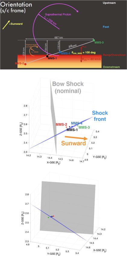
The Astrophysical Journal Letters, 911:L31 (11pp), 2021 April 20                                                                                         Turner et al.

Figure 1. Overview of the event observed by MMS. (a)–(g) Data from the foreshock transient observed by MMS-1 on 2019 January 30, including: (a) magnetic field
vector in GSE coordinates (XYZ in blue, green, and red, respectively) and magnitude (black); (b) ion omnidirectional energy-flux (color, units eV (cm2 s sr eV)−1);
(c) electron density; (d) ion velocity vector in GSE coordinates (XYZ in blue, green, and red, respectively) and magnitude (black); (e) proton gyroradius (color) as a
function of energy and time; (f) proton gyrofrequency; (g) ion inertial length. (h)–(k) Magnetic field vectors and magnitudes from all four MMS spacecraft zoomed in
on the feature of interest in this study.

(Hull et al. 2020), and reconnection along thin, intense,                                                    2. Data and Observations
electron-scale current sheets (Gingell et al. 2019; Liu et al.                           Data from NASAʼs MMS mission (Burch et al. 2016a) are
2020). Upstream of quasi-parallel supercritical shocks, large-                        utilized for this study. MMS consists of four spacecraft that are
scale transient structures can form in the ion foreshock due to                       identically instrumented to study electron-kinetic scale physics of
reflected ions’ kinetic interactions with the turbulent and                            magnetic reconnection (e.g., Burch et al. 2016b; Torbert et al.
discontinuous incident plasma (e.g., Omidi et al. 2010; Turner                        2018). Here, we use data from the fluxgate (Russell et al. 2016)
et al. 2018; Schwartz et al. 2018; Haggerty & Caprioli 2020).                         and search-coil (Le Contel et al. 2016) magnetometers, ion and
Often, new fast magnetosonic shocks form on the upstream                              electron plasma distributions and moments (Pollock et al. 2016),
sides of foreshock transient structures as they expand                                and electric fields (Ergun et al. 2016; Lindqvist et al. 2016).
explosively into the surrounding solar wind and foreshock                             Typically, the four MMS spacecraft are held in a tight tetrahedron
plasmas (e.g., Thomsen et al. 1988; Liu et al. 2016).                                 configuration, with inter-satellite separations of ∼10–100 km.
   State-of-the-art simulations remain computationally limited                        However, during a ∼1 month period in 2019, the spacecraft were
and not yet capable of capturing both true electron-to-ion mass                       realigned into a “string-of-pearls” configuration, in which they
ratios and electron plasma to cyclotron frequency ratios in three                     were separated by up to several hundreds of kilometers along a
dimensions (and thus coupling between those populations is                            common orbit to study turbulence in the solar wind at ion-kinetic
not necessarily accurate). Meanwhile observations are most                            scales. While in both the tetrahedron and string-of-pearls
often limited by single-point observations, resulting in                              configurations, MMS are ideal for disambiguating spatiotemporal
spatiotemporal ambiguity, and/or inadequate temporal resolu-                          features in dynamic space plasmas. With this uncommon MMS
tion. Furthermore, theory and observations (e.g., Morse et al.                        configuration, we examined in detail a foreshock transient event
1972; Krasnoselskikh et al. 2002; Sundberg et al. 2017;                               reported in Turner et al. (2020), which showcased an intriguing
Dimmock et al. 2019; Madanian et al. 2021) indicate that                              evolution of a fast magnetosonic shock.
supercritical shocks undergo periodic reformation, also known                            Figure 1 shows data from the event. Panels (a)–(g) show data
as nonstationarity, which further complicates discerning details                      from MMS-1, highlighting the foreshock transient. The transient,
in single-point observations of well-formed shocks. In this                           associated with the deflection of ion velocity between 04:38:45 and
study, we examined fortuitous multipoint observations during a                        04:39:28 UT in Figure 1(d), was originally classified by Turner
single cycle of shock reformation on the upstream edge of a                           et al. (2020) as a foreshock bubble (e.g., Omidi et al. 2010; Turner
foreshock transient using NASAʼs Magnetospheric Multiscale                            et al. 2013), but upon a more detailed investigation for this study,
(MMS) mission upstream of Earthʼs bow shock.                                          the event may be a hot flow anomaly (e.g., Schwartz et al. 2000).

                                                                                  2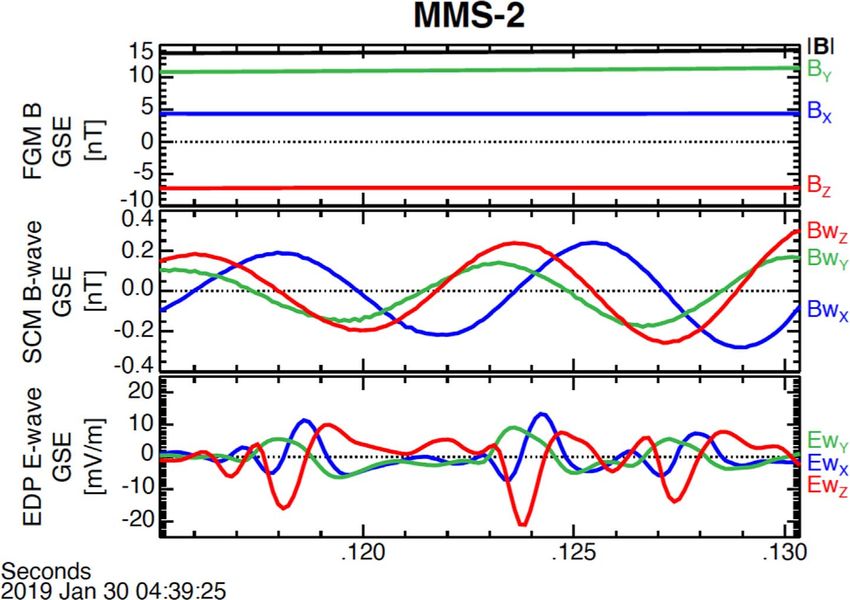
The Astrophysical Journal Letters, 911:L31 (11pp), 2021 April 20 Turner et al.
Evidence supporting this diagnosis consists of the orientation of the transientʼs shock) and estimated at within 0.5 RE of the bow
associated solar wind discontinuity (normal direction, n = [0.69, shock when the foreshock transient was observed.
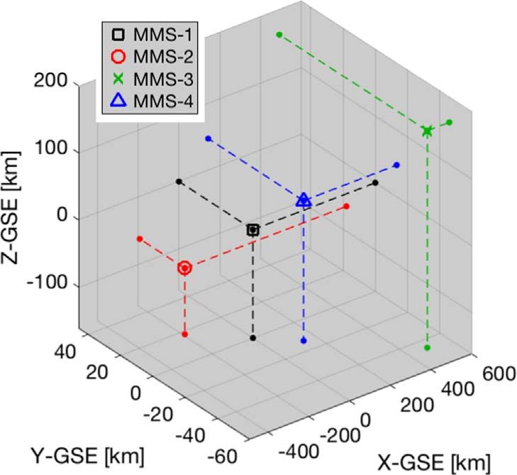
−0.51, −0.52]GSE), which would have already intersected Earthʼs Figure 2(a) shows the relative orientation of the four MMS
bow shock (located ∼0.5 Earth radii, RE, from MMS at the time), spacecraft at 04:39:25UT. MMS-2 was located closest to Earth,
and the orientation of the foreshock transient. More detail on this while MMS-3 was furthest sunward. The four spacecraft were
ion foreshock transient is provided in the next section and the stretched out along the same trajectory with separations ranging
Appendix. For the interest of this study, it is irrelevant whether this from 152 km (MMS-1 to -4) to 723 km (MMS-2 to -3). Those
transient structure was a foreshock bubble or hot flow anomaly, separation scales were comparable to the thermal (and suprather-
since here we are only concerned with the compression region and mal) proton gyroradii in the magnetic fields observed around the
formation of a fast magnetosonic shock on the transientʼs features of interest: a 2 eV (50 eV) proton with pitch angle of 90°
upstream edge. had gyroradius, rcp, of 41, 19, and 10 km (204, 93, and 49 km) in
Figures 1(h)–(k) show magnetic fields observed by all four the 5, 11, and 21 nT B-fields around the “foot,” “ramp,” and
MMS spacecraft between 04:39:15 and 04:39:33 UT. MMS-3 “overshoot” features shown around S = 200, 0, and −50 km in
was the first to pass through the compression region Figure 2(b), respectively. The corresponding proton gyroperiods
(characterized by the enhanced magnetic field strength and were 13, 6, and 3 s, respectively. With the spacecraft locations
plasma densities) on the upstream side of the foreshock projected onto the shock surface, the maximum separation was
transient, followed next by MMS-4, -1, and finally -2. The four 686 km along the shock surface, comparable to the suprathermal
spacecraft observed notable similarities and differences in the rcp in the “foot.” Note that foreshock transients, like hot flow
structure. All four spacecraft observed large-amplitude waves anomalies, are on the order of several Earth radii or larger in size
throughout the compression region; for example, the distinct (e.g., Turner et al. 2013; Liu et al. 2016), much larger than the
peaks in |B| and corresponding oscillations in the B-field MMS separation scales. These are relevant scales to consider for
components observed by MMS-3 between 04:39:19–04:39:24 the following analysis and interpretation.
UT are also evident at the other three spacecraft. However, the With the shock orientation and speed established, it is possible
differences between the four spacecraft observations at the to convert the time series observed by each MMS spacecraft into a
sharp ramp in magnetic field strength (and density) separating spatial sequence, and considering the geometry of the spacecraft
the compression region from the upstream solar wind (e.g., in the system, it is possible to interpret the nature of the observed
around 04:39:24 at MMS-3) are of interest considering spatiotemporal structure. Details for the conversion to spatial
nonstationarity of fast magnetosonic shocks (e.g., Dimmock sequence are included in the Appendix. Results of this conversion
et al. 2019). A new compression signature, first observed by for |B|, density, and current density from MMS are shown in
MMS-3 at 04:39:24 UT then at MMS-4, -1, and -2 at 04:39:26, Figure 2, where the distances have been normalized to an origin
04:39:27, and 04:39:28 UT, respectively, increases in ampl- aligning the features to the initial ramp observed by MMS-3.
itude and duration on the upstream edge. That was the feature When distances are not normalized to align the common features,
that we focused on in detail for this study. the motion of the trailing edge of the foreshock transient,
estimated at ∼120 km s−1 along the shock normal direction
(relative to the initial ramp at MMS-3), shifts the features further
3. Analysis and Results to the right for each subsequent spacecraft crossing after MMS-3
To properly analyze a shock structure, its orientation and speed (see the Appendix). Figure 2(b) shows that each MMS spacecraft
must first be established. Using coplanarity analysis (Schwartz observed similar structure during the crossing and highlights the
1998) with observations of the ramps in |B| observed by all four spatiotemporal evolution of the feature at 10 < S < 70 km that
MMS spacecraft (see the Appendix), a boundary normal was rises up and expands to greater S over time (see also Figures 1(h)–
estimated as [0.54, −0.38, −0.74] ± [0.10, 0.10, 0.10] in GSE 1(k)). We refer to that feature at 10 < S < 70 km as the “new
coordinates. Comparing that normal direction to the upstream shock ramp” structure. With the conversion shown in Figures 2,
B-field, [1.94, 1.16, 0.30]GSE nT, the foreshock transientʼs shock the original shock ramp was located at S ∼ 0 km for all four
was in a quasi-perpendicular geometry with θBN = 80°. From the spacecraft. Key details in Figures 2(c)–2(f) include (i) large-
multipoint crossing and shock normal, the velocity of the shock amplitude B-field waves (note the anticorrelation between |B| and
in the spacecraft frame was [−33.5, 23.5, 45.7] ± [2.1, −1.5, density) at S < 10 km observed by all four spacecraft; (ii) the
−2.9] km s−1 in GSE, which transforms to [207.5, −1.1, largely correlated |B| and density in the new shock ramp structure
−20.5]GSE km s−1 in the solar wind rest frame (using the average observed by all four spacecraft; (iii) the ∼4× jump in magnitudes
upstream solar wind velocity of [−241.0, 24.6, 66.2]GSE km s−1 in of density and |B| in the new shock ramp compared to the
the spacecraft frame). From the four-point observations, the shock upstream conditions at S ∼ 250 km observed by MMS-1 and -2;
speed was increasing with an acceleration of ∼3 km s-2 , which is (iv) oscillations in |B| at 30 < S < 160 km observed by MMS-4,
consistent with the explosive nature of foreshock transients (e.g., −1, and −2; and (v) sharp, narrow current density structures
Turner et al. 2020). The propagation speed in the solar wind frame concentrated primarily along the sharpest gradients in |B| and
is consistent with this structure being a fast magnetosonic shock, density and strongest at S = 0 km.
since the estimated Mach numbers for that propagation speed were Considering the highly correlated nature and time-sequential
MAlfvén = 9.9 and Mfast = 4.2. Note that MMS was ∼5RE growth of the feature referred to as the “new shock ramp”
duskward of the subsolar point of the bow shock at this time, observed in sequence by MMS-3, -4, -1, and -2 during their
and the nominal orientation of the bow shock surface adjacent to crossings of this shock, it is highly unlikely that the feature was
MMS was [0.97, 0.19, 0.13]GSE based on the Fairfield (1971) simply the result of random fluctuations along the 3D shock
model. From the bow shock crossings around the time of interest surface. However, we must consider the possibility that it was a
(not shown), MMSʼs location was in the upstream region of a coherent structure such as a shock surface ripple (e.g., Lowe &
quasi-parallel oriented bow shock (note: not the foreshock Burgess 2003; Johlander et al. 2016; Gingell et al. 2017).
3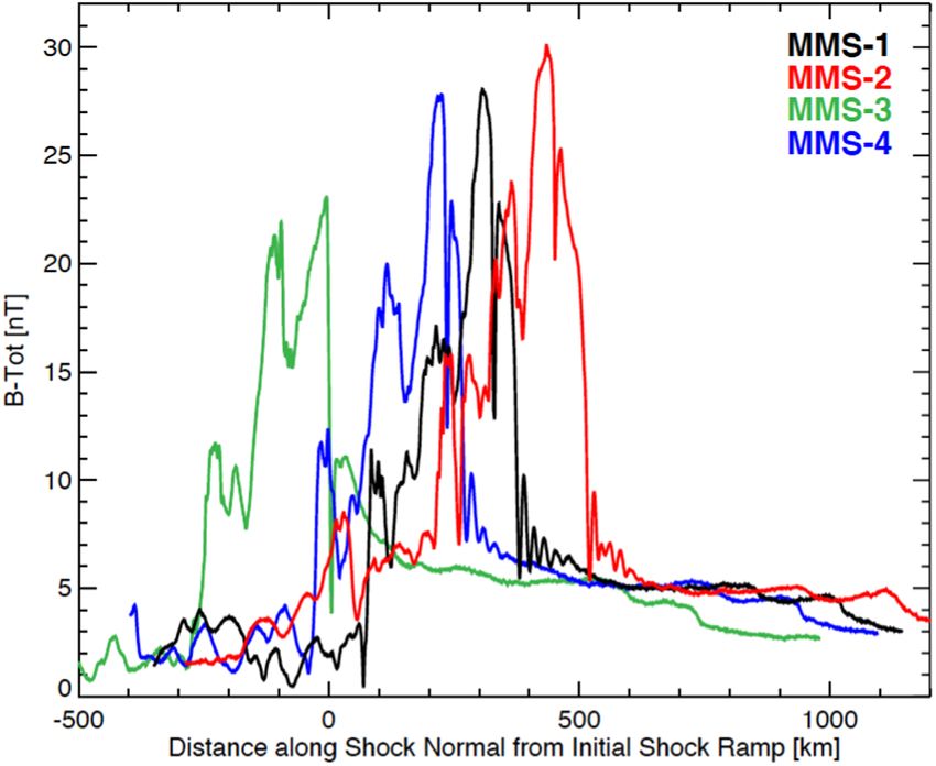
The Astrophysical Journal Letters, 911:L31 (11pp), 2021 April 20                                                                                         Turner et al.

Figure 2. (a) MMS formation in GSE coordinates centered on MMS-1 location, which was at [14.5, 5.1, 2.5] RE in GSE at this time. (b) Magnetic field magnitudes
from all four MMS spacecraft (-1: black, -2: red, -3: green, and -4: blue) plotted along the shock normal direction, S. B-field magnitudes, plasma density, and current
density from MMS-3 (c), -4 (d), -1 (e), and -2 (f). B-fields are shown in the respective spacecraft colors, while density and current density are shown in magenta and
light blue, respectively. Note that current density is unavailable for MMS-4. The original ramp location is indicated with the green arrow in (c), while the new shock
ramp locations are indicated with the corresponding colored arrows for MMS-4, -1, and -2 in (d), (e), and (f), respectively. In panel (c), examples of thermal (2 eV,
dark red) and suprathermal (50 eV, purple) proton gyroradii are shown on the upstream (S > 0) and downstream (S < 0) regimes, as are examples of the ion inertial
length scales (orange) in the upstream regime. Example ion inertial length scales are also shown in the upstream and downstream regimes in (f).

Shock ripples reported along Earthʼs bow shock have                                   A faster growth rate of the new, reforming shock is largely driven
wavelengths of ∼100 to ∼200 km and propagate along the                                by nonlinear steepened waves. These rates have important
shock surface at speeds of ∼65 to ∼150 km s−1 (Johlander                              implications in constraining numerical simulations, which tend
et al. 2016; Gingell et al. 2017). Those wavelengths are                              to yield unrealistic estimates of reformation rates (e.g., Scholer
comparable to the interspacecraft separation of each adjacent                         et al. 2003; Krasnoselskikh et al. 2013).
pair of MMS spacecraft in this event. Assuming comparable                                The large-amplitude waves observed on the downstream side
propagation speeds, a shock surface ripple would pass between                         (S < 0 km) had wavelengths along S comparable to the
MMS-3 and -2 in ∼5–11 s (if propagating perfectly along the                           suprathermal rcp in this frame, and they intensified in amplitude
interspacecraft separation vector) or longer (for different                           closer to S = 0 km. Around S = 0 ± 10 km, the waves were on
propagation directions). The observed timing between the                              electron scales (
The Astrophysical Journal Letters, 911:L31 (11pp), 2021 April 20 Turner et al.
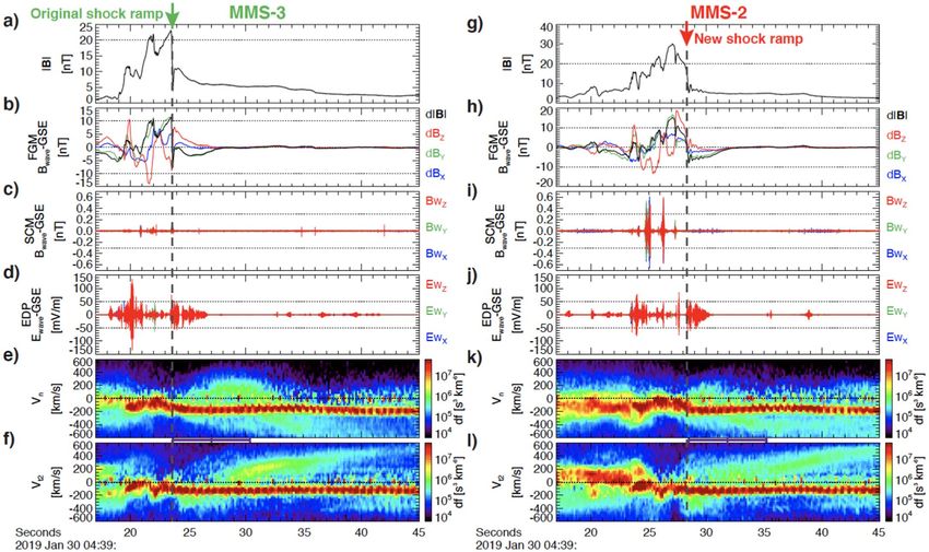
Figure 3. Summary of waves and derived data from MMS-3 (a)–(f) and -2 (g)–(l). For each spacecraft, the following data are plotted: (a) and (g) B-field magnitude
(for ease of comparison with other figures); (b) and (h) low-frequency Bwave (dBi = Bi−⟨ Bi⟩) from the fluxgate magnetometer data in GSE coordinates (dB-XYZ in
blue, green, red, respectively) and d|B| in black; (c) and (i) high-frequency Bwave from the search-coil magnetometer data in GSE coordinates; (d) and (j) high-
frequency Ewave data from the axial and spin-plane double probe data; (e) and (k) ion velocity distributions along the shock normal direction in the shock rest frame; (f)
and (l) ion velocity distributions along a vector perpendicular to the shock normal direction in the shock rest frame, highlighting the incident solar wind beam and
reflected ion gyration. Note that several of the corresponding plots for MMS-2 and -3 are on different Y-scales, so horizontal dashed lines have been put at the same
fixed values on both for ease of comparison.
Figure 3 provides an overview of the electromagnetic and Giagkiozis et al. 2018) were observed in the downstream regime
electrostatic waves and reflected ions observed by MMS during by all four spacecraft, though the amplitude of those whistler-mode
this event. Ion acoustic waves were present upstream of the shock waves increased significantly after the formation of the new shock
observed by all four s/c (-1 and -4 not shown in Figure 3) after ramp; MMS-3 observed lion roars with amplitudes 500 pT (e.g., around 04:39:25.1UT in
shock ramp formed. Strong broadband electrostatic fluctuations, Figure 3(i)). Most interestingly, only at MMS-2 were the lion roars
corresponding to electron-scale nonlinear waves/structures, were also associated with electrostatic solitary waves (ESWs; examples
observed by all four spacecraft, mostly at gradients in B throughout of which are shown in the Appendix), which is important since
the downstream regime, particularly near the boundaries at the new such nonlinear wave decay represents a distinctly irreversible
shock ramp and edge of the HFA core (∼04:29:19UT at MMS-3). energy dissipation process (e.g., Kellogg et al. 2011). In the shock
The nonlinear waves/structures did not occur simultaneously with frame, those ESWs had wavelengths on the order of 100–120 m
the intense, electron-scale current sheets in the downstream regime. along S, approximately one-quarter of the lion roars’ wavelengths
The electrostatic nonlinear waves/structures at MMS-3 extended at ∼460 m along S.
further upstream corresponding with the “foot” structure, whereas Figure 3 also shows ion velocity spectra plotted versus the
for MMS-4, -1, and -2, the fluctuations were limited to shock normal (Vn) and tangential (Vt2) velocity components (e.g.,
approximately the same range in the upstream as the whistler Madanian et al. 2021). Note that Vt2 is by definition perpendicular
precursors, i.e., within ∼1di of the new shock ramp. In the region to the shock normal and upstream B-field vectors. The incident
of the new shock ramp, the amplitude of the electrostatic nonlinear solar wind beam is the high-density population at Vn and Vt2 < 0.
waves/structures was smallest at MMS-3 and largest at MMS-2. The Vt2 distributions clearly show the energy dispersion effect of
The largest-amplitude electrostatic waves/structures, >100 mV ions accelerating and reflecting at the shock ramp: the peak in
m−1, likely corresponded to very short wavelengths ( 0 ions corresponds to higher-energy (larger Vt2) ions
less than the tip-to-tip boom length of the spin-plane electric field completing a half-gyration (after reflection from the ramp in
instruments), which is consistent with observed wavelengths in the |B| ) at increasingly greater distances upstream of the shock. This
shock frame of ∼80–100 m. Those >100 mV m−1 waves were was true for all four spacecraft (see Figures 3(f) and 3(l) for
only observed in the downstream region, S < 0 km, by MMS-3 MMS-3 and −2, respectively), indicating that the shock continues
and -4, not by -1 and -2. Electromagnetic “lion roars” (e.g., to reflect and accelerate suprathermal ions throughout the
5The Astrophysical Journal Letters, 911:L31 (11pp), 2021 April 20 Turner et al.
reformation process. Note also the differences in Vn from MMS-3 precursors just upstream and lion roars throughout the down-
(more intense suprathermal ions at Vn > 0 around 04:39:30UT, stream) waves. Throughout the reformation cycle, the enhanced
corresponding to ∼1 suprathermal rcp from the original shock |B| at the ramp, overshoot, and downstream reflects a significant
ramp, in Figure 3(f)) to MMS-2 (more intense suprathermal ions fraction of incident solar wind ions back into the upstream regime,
at Vn < 0 around 04:39:35UT, corresponding to ∼1 suprathermal resulting in the development of the diamagnetic “foot”-like
rcp from the new shock ramp, in Figure 3(k)), which are possibly structure, out of which the new shock ramp formed. During the
cyclical differences coinciding with the different observed phases reformation process before the new ramp forms, ion-scale waves
of the shock reformation cycle. Those distributions include a steepen and compress in what will ultimately become the new
superposition of ions reflected from the transient structureʼs shock downstream regime. Critically, the compression of the waves
and the main bow shock plus the incident solar wind, and reaches electron-kinetic scales, where strong energy transfer
generation of upstream, ion-scale waves can be associated with then begins along thin, intense current sheets and in the large-
any of these populations plus interactions between them. amplitude, electron-kinetic-scale waves. The compressed waves
and current-sheet energy transfer at electron scales culminate in
the formation of a new shock ramp, with correlated |B| and
4. Summary and Conclusion
density, out of the preexisting “foot”-like structure upstream of the
At 04:39 UT on 2019 January 30, MMS was fortuitously most intense, thin current layer. Once formed, the new shock
positioned to capture what was likely at least half of the ramp and “foot” region continue converting energy of the incident
reformation cycle of a fast magnetosonic shock on the upstream ion and electron populations via whistler-mode precursor and
edge of a transient structure in the quasi-parallel foreshock electrostatic fluctuations within a few di upstream of the shock
upstream of Earthʼs bow shock. Evidence was provided ramp, dissipative wave-mode-coupling downstream of the ramp,
supporting that it was unlikely that the observed features resulted and along thin current layers that may also be reconnecting (e.g.,
from either random fluctuations or shock surface ripples when the Gingell et al. 2019; Liu et al. 2020). As we know from many
spacecraft separation tangential to the shock normal was also observations of foreshock transient shocks, the extent of the
accounted for. This unique case study offered an opportunity to shocked plasma then must expand rapidly back up to ion-kinetic
study the spatiotemporal nature of early shock development in and ultimately MHD scales.
microscopic detail. Calculated shock growth rates indicated that
the new shock ramp grew faster (2.55 nT s−1) than the old shock The authors are thankful to the MMS team for making their
ramp (1.63 nT s−1). As the new shock ramp formed from the data available to the public. We thank the ACE, Wind, and OMNI
“foot” of the preexisting shock, several additional distinct teams and data providers for solar wind data. We are also thankful
differences were observed down to electron-kinetic scales, to the anonymous reviewer for constructive suggestions and
including intensification of electron-scale waves, nonlinear comments. Funding support for several authors was via the MMS
waves/structures, and intense current sheets. It was at those mission, under NASA contract NNG04EB99C, and research
electron-kinetic scales (∼1di). tional Teams program. D.L.T. is also thankful for funding from
Prior to the shock ramp reforming, the steepened, large-amplitude NASA grants (NNX16AQ50G and 80NSSC19K1125). S.J.S.
ion-scale wavefronts were also affecting electrons, resulting in the was supported in part by a subcontract from Univ. of New
growth of electrostatic and electromagnetic wave modes and thin, Hampshire on NASA award 80NSSC19K0849. H.M. was
intense current layers. However, once the new shock ramp was supported in part by NASA grant 80NSSC18K1366. H.H. was
properly established, as exemplified by MMS-2, both the supported by the Royal Society University Research Fellowship
electrostatic and electromagnetic waves amplified significantly at URF\R1\180671. The French LPP involvement for the SCM
the new shock ramp and in the downstream region. The most instrument was supported by CNES and CNRS. SPEDAS
intense current layer was observed along the original shock ramp software (Angelopoulos et al. 2019) was used to access, process,
(around S = 0 km), and the new shock ramp and an overshoot and analyze the MMS data. MMS data used in this study are
formed immediately upstream and downstream of that intense, available at https://lasp.colorado.edu/mms/sdc/public/.
electron-scale current layer, respectively. Note that the overshoot
on the downstream side of the current layer was likely that of the Appendix
original shock ramp, and from the available snapshots of the new Supporting Material
ramp, it is difficult to identify where any new overshoot was
A.1. Calculating the Local Bow Shock Orientation
formed. Only after the new shock ramp formed were whistler
precursors in the upstream region and potentially dissipative Local bow shock normal direction from the Fairfield (1971)
wave–wave interactions in the downstream region observed. All model
combined, the results indicate that a shockʼs energy conversion
and dissipation processes may also undergo the same cyclical nbs = [0.974, 0.190, 0.127] in GSE,
periodicity as reformation of the shock front. Upstream magnetic field (average from MMS-1)
This special case exemplifies the genuine cross-scale coupling
that occurs between the ion- and electron-kinetic physics at B = [2.00, 2.37, 0.35] nT in GSE.
collisionless, fast magnetosonic shocks. The ions, with their large
Angle between bow shock normal and upstream B-field
gyroradii, enable information transfer “very far” (with respect to
electron scales) into both the upstream and downstream regimes, q Bn = 38.5.
but the key physics for energy dissipation and heating occur at
least in some relevant part at electron scales via thin, intense, So MMS were in the quasi-parallel foreshock, consistent with
electron-scale current sheets and large-amplitude, nonlinear plasma and field observations and the presence of the foreshock
electrostatic fluctuations and electromagnetic (e.g., whistler transient structure.
6The Astrophysical Journal Letters, 911:L31 (11pp), 2021 April 20 Turner et al.
A.2. Calculating the Foreshock Transient’s Shock Normal Average shock speed along shock normal ± 1 standard
Direction and Orientation deviation
Using coplanarity with B and V from Schwartz (1998),
Vsh = - 62.1 1.9 km s-1.
n = (DB ´ DV ´ DB) ∣(DB ´ DV ´ DB)∣
whereDX = Xdownstream - Xupstream , X = BorV . Note that the shock is apparently accelerating along the shock
Table A1 normal direction at an average rate of
Results from Coplanarity Analysis to Calculate Shock Normal
a = 2.93 km s-2.
Downstream Upstream
Coplanarity Times Times n-GSE
B and V 04:UT+ 04:UT+ Shock velocity in spacecraft frame (GSE)
MMS-1 39:24.0–39:26.0 39:30.0–39:32.0 [0.389,
−0.315, −0.866]
Vsh∣sc = [ - 33.5, 23.5, 45.7] [2.1, - 1.5, - 2.9] km s-1.
MMS-2 39:25.0–39:27.0 39:31.0–39:33.0 [0.590,
−0.551, −0.620] Shock velocity in solar wind frame (GSE)
MMS-3 39:20.5–39:23.0 39:27.0–39:29.0 [0.670,
−0.338, −0.661] Vsh∣sw = [207.5, - 1.1, - 20.5] [2.1, - 1.5, - 2.9] km s-1.
MMS-4 39:22.5–39:25.3 39:28.0–39:30.0 [0.512,
−0.313, −0.800]
Mach numbers in background solar win are
Average n from all four s/c ± 1 standard deviation on the MAlfveń = 9.9, Mfast = 4.2.
mean
nsh = [0.540, - 0.379, - 0.737] [0.104, 0.010, 0.100] in GSE. A.3. Converting MMS Time Series to Distance along Shock
Normal Vector
Magnetic field upstream of the transientʼs shock
VMMS∣sh = VMMS - Vsh: MMS velocity in shock reference frame
B = [1.94, 1.16, 0.30] nT in GSE. vMMS∣sh = VMMS∣ sh.nsh : MMS apparent speed along shock normal
Angle between transient shock normal and upstream B-field
q Bn = 80.3. t3(0): time at which MMS-3 observed the original shock ramp
(see “Shock Ramp t” in Table A2)
So the transient shock was in a quasi-perpendicular orientation.
Dti = ti (t ) - ti (0) , i = {1, 2, 3, 4},
Table A2
Calculating the Foreshock Transientʼs Shock Speed DSi = v MMS∣sh * Dti.
Shock Velocity (km For each spacecraft, i = {1, 2, 3, 4}, ΔSi is then the distance
Spacecraft Ramp t Location in GSE (km) s−1) along the shock normal direction from the original shock ramp
MMS-1 04:39:26.320 [92772.145, 32264.144, [−1.715, location; thus, S = 0 is where each MMS spacecraft first
UT 16086.952] 0.155, −0.562] observed the original shock ramp.
MMS-2 04:39:27.310 [92579.885, 32282.023, [−1.719, Note that for the results shown in Figure 2, S was calculated
UT 16023.796] 0.154, −0.563] using ti(0) for each spacecraft. See Figure A1 for example of
MMS-3 04:39:23.600 [93264.432, 32218.352, [−1.704, the spatial series plotted versus S where all four spacecraft are
UT 16248.785] 0.159, −0.560]
referenced to the location (S = 0) of the original shock ramp
MMS-4 04:39:25.550 [92915.644, 32250.873, [−1.712,
UT 16134.104] 0.156, −0.561]
when/where it was first observed by MMS-3 at t3(0). That
conversion showcases the expansion speed of the foreshock
transient but does not align common features between all four
* Δt = ΔX. nsh. spacecraft.
Shock speed Vsh
Table A3 A.4. Foreshock Transient Shock Orientation Sketches
Estimates of Shock Speed between Different Spacecraft Pairs
Figure A2 shows a cartoon sketch of the orientation of the
MMS spacecraft with respect to the observed shock. These
Spacecraft |ΔX| Δt Shock Speed
Pairs (km) (s) (km s−1)
viewpoints offer context for how the shock was oriented,
passed over and was observed by each of the four MMS
MMS-3 to -4 368.6 1.94 −59.9 spacecraft, and some relative scale sizes (e.g., the spacecraft
MMS-3 to -1 520.2 2.72 −60.5 separations with respect to thermal and suprathermal ion
MMS-3 to -2 723.4 3.70 −61.7 gyroradii). The bottom portions of Figure A2 also show two
MMS-4 to -1 151.6 0.78 −61.7 perspectives on how the observed shock was oriented with
MMS-4 to -2 354.8 1.79 −63.6
respect to the local bow shock location, estimated based on the
MMS-1 to -2 203.2 0.99 −65.1
MMS observations as described in the main text.
7The Astrophysical Journal Letters, 911:L31 (11pp), 2021 April 20 Turner et al.
Figure A1. |B| time series from each MMS spacecraft converted to distance along shock normal direction using t3(0) for all four spacecraft, i.e., instead of ti(0). This
conversion captures the expansion of the foreshock transient but does not align common features along this version of S.
8The Astrophysical Journal Letters, 911:L31 (11pp), 2021 April 20 Turner et al.
Figure A2. Sketches of the orientation and relative size scales of the foreshock transient shock and MMS spacecraft and the bow shock.
9The Astrophysical Journal Letters, 911:L31 (11pp), 2021 April 20 Turner et al.
Figure A3. Example of possible nonlinear wave decay on electron-kinetic scales. From top to bottom, the three panels show the magnetic field vector in GSE (XYZ in
blue, green, and red) and magnitude (black), Bwave in GSE coordinates from the search-coil magnetometer, and Ewave in GSE coordinates from the electric field double
probes. The middle panel shows approximately two wavelengths from an electromagnetic whistler-mode “lion roar” observed by MMS-2 in the downstream plasma
regime, while the bottom panel shows three large-amplitude electrostatic solitary waves.
A.5. High-resolution Electrostatic Wave Observations Ergun, R. E., Tucker, S., Westfall, J., et al. 2016, SSRv, 199, 167
Fairfield, D. H. 1971, JGR, 76, 6700
Figure A3 shows electrostatic waves (ESWs) observed Ghavamian, P., Schwartz, S. J., Mitchell, J., Masters, A., & Laming, J. M.
associated with whistler-mode lion roars by MMS-2. One 2013, SSRv, 178, 633
possibility is that the ESWs result from nonlinear wave Giagkiozis, S., Wilson, L. B., Burch, J. L., et al. 2018, JGRA, 123, 5435
Gingell, I., Schwartz, S. J., Burgess, D., et al. 2017, JGRA, 122, 11,003
decay, but with these observations alone, it is impossible to Gingell, I., Schwartz, S. J., Eastwood, J. P., et al. 2019, GeoRL, 46, 1177
rule out simultaneous, coincidental occurrence. We simply Goodrich, K. A., Barabash, S., Futaana, Y., et al. 2019, JGRA, 124, 4104
note this here for interest and leave detailed analysis for future Goodrich, K. A., Ergun, R., Schwartz, S. J., et al. 2018, JGRA, 123, 9430
studies. Gosling, J. T., & Robson, A. E. 1985, GMS, 35, 141
Haggerty, C. C., & Caprioli, D. 2020, ApJ, 905, 1
Hull, A. J., Muschietti, L., Le Contel, O., Dorelli, J. C., & Lindqvist, P.-A.
ORCID iDs 2020, JGR, in press
Johlander, A., Schwartz, S. J., Vaivads, A., et al. 2016, PhRvL, 117,
D. L. Turner https://orcid.org/0000-0002-2425-7818 165101
L. B. Wilson, III https://orcid.org/0000-0002-4313-1970 Kellogg, P. J., Cattell, C. A., Goetz, K., Monson, S. J., & Wilson, L. B., III
H. Madanian https://orcid.org/0000-0002-2234-5312 2011, JGRA, 116, A09224
T. Z. Liu https://orcid.org/0000-0003-1778-4289 Kozarev, K. A., Korreck, K. E., Lobzin, V. V., Weber, M. A., &
Schwadron, N. A. 2011, ApJL, 733, L25
A. Johlander https://orcid.org/0000-0001-7714-1870 Krasnoselskikh, V., Balikhin, M., Walker, S. N., et al. 2013, SSRv, 178, 535
D. Caprioli https://orcid.org/0000-0003-0939-8775 Krasnoselskikh, V., Lembege, B., Savioni, P., & Lobzin, V. V. 2002, PhPl,
I. J. Cohen https://orcid.org/0000-0002-9163-6009 9, 1192
D. Gershman https://orcid.org/0000-0003-1304-4769 Le Contel, O., Leroy, P., Roux, A., et al. 2016, SSRv, 199, 257
Lindqvist, P.-A., Olsson, G., Torbert, R. B., et al. 2016, SSRv, 199, 137
J. H. Westlake https://orcid.org/0000-0003-0472-8640 Liu, T. Z., Lu, S., Turner, D. L., et al. 2020, JGRA, 125, e27822
B. Lavraud https://orcid.org/0000-0001-6807-8494 Liu, T. Z., Turner, D. L., Angelopoulos, V., & Omidi, N. 2016, JGRA,
O. Le Contel https://orcid.org/0000-0003-2713-7966 121, 5489
J. L. Burch https://orcid.org/0000-0003-0452-8403 Lowe, R. E., & Burgess, D. 2003, AnGeo, 21, 671
Madanian, H., Desai, M. I., Schwartz, S. J., et al. 2021, ApJ, 908, 40
Masters, A., Stawarz, L., Fujimoto, M., et al. 2013, NatPh, 9, 164
References Morse, D. L., Destler, W. W., & Auer, P. L. 1972, PhRvL, 28, 13
Omidi, N., Eastwood, J. P., & Sibeck, D. G. 2010, JGRA, 115, A06204
Angelopoulos, V., Cruce, P., Drozdov, A., et al. 2019, SSRv, 215, 9 Pollock, C., Moore, T., Jacques, A., et al. 2016, SSRv, 199, 331
Breuillard, H., Le Contel, O., Chust, T., et al. 2018, JGRA, 123, 93 Russell, C. T., Anderson, B. J., Baumjohann, W., et al. 2016, SSRv, 199, 189
Burch, J. L., Moore, T. E., Torbert, R. B., & Giles, B. L. 2016a, SSRv, 199, 5 Scholer, M., Shinohara, I., & Matsukiyo, S. 2003, JGRA, 108, 1014
Burch, J. L., Torbert, R. B., Phan, T. D., et al. 2016b, Sci, 352, aaf2939 Schwartz, S. J. 1998, in Analysis Methods for Multi-spacecraft Data, ed.
Caprioli, D., Pop, A.-R., & Spitkovsky, A. 2015, ApJL, 798, L28 G. Paschmann & P. W. Daly (Noordwijk: ESA), 1
Caprioli, D., & Spitkovsky, A. 2014a, ApJ, 783, 91 Schwartz, S. J., Avanov, L., Turner, D., et al. 2018, GeoRL, 45, 11,520
Caprioli, D., & Spitkovsky, A. 2014b, ApJ, 794, 46 Schwartz, S. J., Paschmann, G., Sckopke, N., et al. 2000, JGR, 105, 12639
Chen, L.-J., Wang, S., Wilson, L. B., et al. 2018, PhRvL, 120, 225101 Sundberg, T., Li, B., Chen, S.-X., et al. 2017, ApJ, 836, 1
Cohen, I. J., Schwartz, S. J., Goodrich, K. A., et al. 2018, JGRA, 124, 3961 Thomsen, M. F., Gosling, J. T., Bame, S. J., et al. 1988, JGR, 93, 11311
Dimmock, A. P., Russell, C. T., Sagdeev, R. Z., et al. 2019, SciA, 5, eaau9926 Torbert, R. B., Burch, J. L., Phan, T. D., et al. 2018, Sci, 362, 1391
Eastwood, J. P., Lucek, E. A., Mazelle, C., et al. 2005, SSRv, 118, 41 Turner, D. L., Liu, T. Z., Wilson, L. B., et al. 2020, JGRA, 125, e27707
10The Astrophysical Journal Letters, 911:L31 (11pp), 2021 April 20 Turner et al.
Turner, D. L., Omidi, N., Sibeck, D. G., & Angelopoulos, V. 2013, JGRA, Wilson, L. B., III, Koval, A., Szabo, A., et al. 2012, GeoRL, 39, L08109
118, 1552 Wilson, L. B., III, Sibeck, D. G., Breneman, A. W., et al. 2014a, JGRA,
Turner, D. L., Wilson, L. B., Liu, T. Z., et al. 2018, Natur, 561, 206 119, 6455
Viñas, A. F., & Scudder, J. D. 1986, JGR, 91, 39 Wilson, L. B., III, Sibeck, D. G., Breneman, A. W., et al. 2014b, JGRA,
Wilson, L. B., III, Cattell, C., Kellogg, P. J., et al. 2007, PhRvL, 99, 041101 119, 6475
11You can also read