Do Credit Rating Agencies Add Value? Evidence from the Sovereign Rating Business Institutions
←
→
Page content transcription
If your browser does not render page correctly, please read the page content below
Inter-American Development Bank
          Banco Interamericano de Desarrollo (BID)
                    Research Department
                Departamento de Investigación
                    Working Paper #647

Do Credit Rating Agencies Add Value?
 Evidence from the Sovereign Rating
        Business Institutions
                            by

            Eduardo A. Cavallo*
              Andrew Powell*
             Roberto Rigobón**

      **Inter-American Development Bank
    **Massachusetts Institute of Technology

                   November 2008
Cataloging-in-Publication data provided by the
Inter-American Development Bank
Felipe Herrera Library
Cavallo, Eduardo A.
Do credit rating agencies add value? : evidence from the sovereign rating business
institutions / by Eduardo A. Cavallo, Andrew Powell, Roberto Rigobón.
p. cm. (Research Department Working Papers ; 647)
Includes bibliographical references.
1. Credit bureaus. 2. Credit control. I. Powell, Andrew (Andrew Philip). II. Rigobón,
Roberto. III. Inter-American Development Bank. Research Dept. IV. Title. V. Series.
HG3751.5 .C234 2008
332.7 C234-----dc22
©2008
Inter-American Development Bank
1300 New York Avenue, N.W.
Washington, DC 20577
The views and interpretations in this document are those of the authors and should not be
attributed to the Inter-American Development Bank, or to any individual acting on its behalf.
This paper may be freely reproduced provided credit is given to the Research Department, Inter-
American Development Bank.
The Research Department (RES) produces a quarterly newsletter, IDEA (Ideas for Development
in the Americas), as well as working papers and books on diverse economic issues. To obtain a
complete list of RES publications, and read or download them please visit our web site at:
http://www.iadb.org/res.
2Abstract1
If rating agencies add no new information to markets, their actions are not a
public policy concern. But as rating changes may be anticipated, testing whether
ratings add value is not straightforward. This paper argues that ratings and spreads
are both noisy signals of fundamentals and suggest ratings add value if,
controlling for spreads, they help explain other variables. The paper additionally
analyzes the different actions (ratings and outlooks) of the three leading agencies
for sovereign debt, also considering the differing effects of more or less
anticipated events. The results are consistent across a wide range of tests. Ratings
do matter and hence how the market for ratings functions may be a public policy
concern.
JEL Codes: F37, G14, G15, C23
Keywords: Ratings, Spreads, Information Economics, Event Studies.
1
This paper represents the views of the authors and do not necessarily reflect the views of any institution including
the IDB, its Executive Directors or the countries they represent. We thank Jeromin Zettelmeyer, John Chambers,
Eduardo Fernández-Arias and seminar participants at the XXVII Meeting of the Latin American Network of Central
Banks and Finance Ministries for very useful comments and Francisco Arizala for superb research assistance. All
remaining errors are our own.
31. Introduction
Recently, rating agencies have come under fire for their role in assessing risks of structured
products. Here we focus on something they have been doing for a longer period of time: rating
sovereign debt. Debt instruments are actively traded in secondary markets, thereby providing
up-to-date information on prices, yields and spreads over riskless debt. Credit ratings are often
mapped into default probabilities, but bond spreads may also be mapped onto the same scale.
Credit ratings and spreads appear, then, to be capturing the same thing; the question we consider
in this paper is what can rating agencies tell us that we cannot learn simply from looking at the
price of debt?
One potential answer is that rating agencies and investors may have different information
sets. Take the case of a small investor who wishes to have a diversified portfolio. It would
generally not be in the interests of each such investor to have a large research department
focusing on the fundamentals of each country. Instead, the investor will rely on a central
information source such as a rating agency. Some larger investors may of course have research
departments, and brokers that serve many investors are also a source of a great deal of analysis.
A second answer is that investors and rating agencies with the same information may have
different opinions. Indeed, as we detail below, different rating agencies frequently have different
views on sovereigns. Roughly, and using standard mappings between the agencies, they disagree
about as much as they agree on ratings. Another way to state the potential role of rating agencies
is then to suggest that ratings and spreads are both noisy signals of true and perhaps unknowable
deep economic fundamentals. The question we address in this study is, then, given the signals
provided by markets, do rating agencies add information?
This is an important topic not only as an academic issue to understand how markets
function, including the market for information on how to value assets, but also an important
policy issue. If rating agencies do not add information, then their opinions do not matter and it is
difficult to argue that there is any policy concern regarding their activities. On the other hand, if
it is found that they do add information, their opinions matter and it is important to know that the
credit rating market is working well.
Several recent papers have considered the role of rating agencies in the sovereign debt
market. Cantor and Packard (1996) and Afonso, Gomes and Rother (2007) show that ratings can
be modeled fairly successfully by economic fundamentals. Several papers show that ratings
4affect spreads, but the real question is whether ratings affect spreads controlling for
fundamentals. Eichengreen and Mody (1998) and Dell’Ariccia, Schnabel and Zettelmeyer (2006)
regress ratings on fundamentals and interpret the error as the rating agencies’ “opinion.” They
then show that this residual is highly significant in explaining spreads. Powell and Martínez
(2007) replicate these analyses; they also employ a system of equation approach and further
argue that the rating agencies’ differences in opinion are informative. In other words, when one
agency changes a rating and the others do not, then this is associated with a change in spreads.
Despite these efforts, it is not yet possible to argue that the case is closed. Each
methodology employed to date has its particular drawbacks. In the case of the technique used by
Eichengreen and Mody (1998) and Dell’Ariccia et al. (2006), it is a heroic assumption that the
error of the ratings equation represents the rating agencies’ opinion and not that this equation is
simply mis-specified. In the system approach favored by Powell and Martinez (2007) a different
but also heroic assumption is needed to identify the system. In the approach employing rating
agencies’ differences of opinions, one rating agency may follow a spread change rather than
actually affect the spread. Moreover, there may be more information in markets than is captured
in these models, and the above approaches do not control for the current information in markets,
but only current fundamentals and/or ratings. This paper raises the bar with respect to the papers
cited by testing if credit ratings influence spreads over and above the information that is already
aggregated in market variables.
Another tack would be to attempt an event study as in the corporate finance literature—
see Campbell, Lo and Mckinlay (1997) for a discussion. However, rating agencies appear to try
to signal when rating changes may occur. Sovereign debt is either given a positive or negative
outlook (suggesting an upgrade or a downgrade may be the next change respectively) and
additionally may be placed on a “rating watch” (indicating that a decision may be about to be
made). Moreover, agencies publish what a particular sovereign would have to do to improve its
rating, and while targets may not be precise, the information required to make a judgment is
generally public and indeed may become a focus of market research and analysis. All this
implies that the classic event study methodology may not be appropriate as rating changes may
be anticipated.
This means that it is a real challenge to answer the question as to whether ratings
agencies add value. If rating agency actions are fully anticipated then we would see no effect on
5spreads. But seeing no effect on spreads of a rating change would not mean that rating agencies
do not add value. In our view outlined above, that both ratings and spreads are noisy signals of
fundamentals, it just implies that whatever effect ratings had on spreads may have already been
incorporated into spreads. We therefore suggest that we need to seek other methods to tackle
this question.
For this purpose, we first devise a simple specification test to evaluate whether or not
ratings are informative. We conclude that they are. Next, we consider a type of horse race
between ratings and spreads as to how well they are correlated to other macroeconomic variables
using high-frequency data. We suggest that, given the possibility of full anticipation, this is a
better method to evaluate whether rating agencies add value.
However, we also argue that outlook changes give interesting information on how
anticipated rating changes have been. If the outlook is changed just a few days before the rating,
then it seems reasonable to suggest that the rating change is largely unanticipated before that
date. We exploit this and other further details of the process in our analysis below.
We also conduct tests on whether certain rating changes are more important that others.
In particular, if a debt issue obtains an “investment grade” rating this may allow different classes
of investors to purchase those issues and hence the instrument may be said to have changed
“asset class.” We test below whether rating changes in and out of investment grade are more
important than other changes.
Our results across several methods and for the three main credit rating agencies are strong
and highly consistent. We find that we cannot reject the view that rating agencies add value. We
find that this is true for both changes in asset classes and other rating changes, and we find that
less anticipated rating changes have even more significant effects. We conclude that rating
agencies do matter, and hence that there is a public policy concern regarding whether these
agencies are doing a good job.
62. Organizing Framework
The question we are interested in answering is to evaluate the informational content that the
rating has in addition to the observed spread on marketable sovereign debt (henceforth spread).2
In other words, the null hypothesis that all the information in the rating is already reflected in the
spread is equivalent to saying that the spread is a sufficient statistic. The alternative hypothesis,
on the other hand, implies that spreads and ratings are imperfect measures of the unobservable
fundamentals of the economy, and therefore ratings provide information above and beyond what
spreads reflect.
In this section we organize our thoughts regarding ratings and spreads in a simple error-
in-variables framework. The goal is to devise a simple specification test to evaluate whether or
not ratings are informative.
2.1 Preliminary Considerations
Some considerations are necessary to clarify before devising an empirical strategy. First, this
paper is studying sovereign ratings, and in this context rating agencies are concerned with
evaluating countries’ probability of default, or country risk. This is important because in this
environment, if the spread of the sovereign debt is observed, then it is reasonable to assume that
the spread and the rating are supposedly capturing the same aspect.
It is impossible to evaluate the informational content in the rating only using ratings and
spreads. We need other variables. Fortunately, country risk not only affects the spread, but also
impacts other macroeconomic variables. For instance, an increase in the probability of default of
a country should have a negative impact on all asset prices, particularly stock prices. Therefore,
if we observe a downgrade we should expect a drop in the stock market index. If the spread is a
sufficient statistic for the rating, then if we were to run a regression where the spread and the
rating are included on the RHS, the rating should be insignificant after controlling for the spread.
In fact, we study three macro variables: the spread one period ahead, stock market prices, and the
nominal exchange rate.
2
We focus the analysis on sovereign bonds spreads, which are computed as the difference of the yield-to-maturity of
a bond, minus the yield-to-maturity of a comparable riskless bond (i.e., US Treasuries). These are the most widely
used proxies of risk by market observers.
7The second consideration is that we concentrate on high-frequency (i.e., daily) data. This
explains our choice of macro variables. The main reason why we look at daily data is that, if
ratings have any informational content beyond the spread, we expect this information to be
incorporated into macro variables within days; and therefore, monthly data will be unable to
disentangle the spread and the ratings informational components.
Third, if ratings and spreads are imperfectly measuring the fundamental—default
probability—then we can interpret them as noisy versions of an unobservable fundamental.
However, the rating, because of its discrete nature, is then a version of the fundamental whose
noise is not of classical form. In other words, the rating can be interpreted as a discretization of
the fundamental, and the noise implied in this measure is serially correlated, and correlated with
the fundamental—hence making it a non-classical error-in-variables problem. Our methodology
testing for the informational content has to be robust to this property of the data. Furthermore,
ratings are very sticky, in the sense they change very infrequently when observed daily. This
means that the error-in-variables (EIV) problem in the rating is probably more severe than in the
spread estimation. Therefore, in horse race estimations between the spread and the rating we
have to be careful to take into account the possibility that the EIV biases are different across the
two variables.
Fourth, exchange rates, spreads, stock prices, and ratings are all endogenous. The
methodology we devise has to take into consideration that linear regressions might be mis-
specified. The test has to be meaningful even in the presence of other forms of mis-specification
(not just the error-in-variable interpretation). More importantly, a crucial form of endogeneity is
the fact that credit rating changes are indeed anticipated by market participants. This not only
affects the interpretation but also how to implement the estimation. We return to the point of
anticipation later in the results section.
2.2 Specification Test
With these four considerations at hand, we now proceed to explain our empirical strategy. We
assume that spreads ( it ) and ratings ( rt ) are noisy versions of an unobserved fundamental,
it = i0 + θxt + ε t
rt = r0 + f ( xt ,η t )
8where the idea is that xt is the unobserved fundamental that not only affects the probability of
default of the country (and its spread) but also affects the exchange rate, stock markets, and
future spreads. We assume that the rating is a non-linear function of the fundamental—trying
trying to emphasize the discreteness of the variable. We assume a simple linear function for the
spread, although that is not restrictive.
Assume that another macroeconomic variable y t (which for expositional simplicity let’s
assume it is the stock market) is affected by the same fundamental,
y t = y 0 + β xt + μ t
The null hypothesis is that the spread is a sufficient statistic—i.e., that the rating does not
add information beyond what the spread already captures. In a well-specified regression we
could test for this by just running a horse race between spreads and rating. However, if the
variables are endogenous or they are measured with error, then this simple procedure might not
produce the correct inference.
To resolve this problem we take several steps in the estimation procedure. First, we
concentrate on the relationship between macro variables, spreads and ratings around the periods
in which the rating changes. Our preferred specification looks at the window 10 days before and
after a credit rating is modified. Second, we compute the cumulative return on all the variables
over the events windows. This means that if the movement in the rating is anticipated, spreads
and macro variables will adjust before the rating actually changes. Hence, all will be
endogenously determined. Third, in this environment, we regress the cumulative change in the
macro variables on the spread and compare the estimates when the spread is instrumented by the
rating. If the spread is a sufficient statistic for the rating, the two coefficients should be similar. If
the spread and the rating summarize different sets of information—i.e. both are imperfect
measures of the fundamentals—then the two coefficients will be statistically different.
This procedure is robust to misspecification of the macro variable on the spread
regression. In other words, when we say that the spread is a sufficient statistic for the rating,
technically what we are saying is that the change in the rating is captured by the movement of the
spread, and everything else in the rating is just noise. Instrumenting the spread with the rating
around the window in which the rating is changing therefore implies that both capture the same
change in fundamentals. By concentrating on the window around the rating change we are
9minimizing the EIV in the rating measure and providing the best chance to the rating to provide
additional information.3
What means that the spread is a sufficient statistic for the rating? The simple model
below highlights a case in which the spread is indeed a sufficient statistic.
it = i0 + θxt
rt = r0 + f ( xt ,η t )
y t = y 0 + β xt + μ t
2.2.1 Uncorrelated Error-in-Variables and Exogenous Fundamentals
Let us start by studying the case when all the residuals are uncorrelated. Because the spread
captures the information in the fundamental perfectly, when we estimate the regression:
y t = c0 + bit + ϕ t
the OLS estimate is consistent. Because the rating is a noisy version of the same fundamental,
and its noise is uncorrelated with the residual in the stock market equation, then if we instrument
the spread with the rating we also estimate a consistent coefficient. Importantly, the instrumental
variable estimate is inefficient under the null hypothesis, and OLS is efficient.
Under the alternative hypothesis the spread is a noisy version of the fundamental. This
means that the OLS estimate is inconsistent and biased; the bias comes exactly from the noise.
This estimate can be improved, however, and the rating is a perfect instrument for doing so.
First, it is correlated with the spread because both are measures of the same fundamental.
Second, their noises are different, and such noises are uncorrelated with the fundamentals. This
means that the rating is uncorrelated with the residual in the stock market regression. In other
words, the rating is a valid instrument for the spread and the IV estimates are going to be a
consistent estimate of the true parameter.
This is a standard specification test. Under the null hypothesis, OLS is consistent and
efficient, while IV is consistent but inefficient. On the other hand, under the alternative
hypothesis, OLS is inconsistent, but IV continues to be consistent (see Hausman, 1978).
3
In other words, when the rating is not changing it is possible to argue that the default probability is changing little
as well, and therefore no change in ratings is imperfectly measuring small changes in fundamentals. However, when
the rating is indeed changing, we expect in those windows for the fundamental to cross some threshold, and
therefore the increase in the rating indeed reflects an improvement in the fundamental.
102.2.2 Uncorrelated error-in-variables, and endogenous fundamentals
The most important source of possible misspecification in this model is when the fundamentals
are not exogenous—in other words, when cov( xt , μ t ) ≠ 0 .
The methodology we have described has no problems dealings with this form of
misspecification. Let us assume that the measured fundamental and the residual in the stock
market equation are correlated. The implication of this assumption is that OLS is biased, but
because in our window the rating is proportional to the fundamental xt , then the IV will be
equally biased if and only if the spread is a sufficient statistic. In other words, if the spread is a
sufficient statistic but the fundamentals are correlated with the residual in the macro equation,
OLS and IV are equally biased. In the alternative hypothesis, when the spread is not a sufficient
statistic, then both coefficients are biased, but they are biased differently.
The simplest way to understand the intuition behind this test is to assume that both the
spread and the rating are linear functions of the fundamental:
it = i0 + θxt
rt = r0 + αxt + η t
y t = y 0 + β xt + μ t
The OLS estimate of the stock market on the spread is equal to
cov(it , y t ) βθ var( xt ) + θ cov( xt , μ t ) β cov( xt , μ t )
bˆOLS = = = +
var(it ) θ 2 var( xt ) θ θ var( xt )
where, just for clarification, the bias arises from the correlation between the fundamental and the
residual in the stock market regression. It is needless to say that the OLS estimate—when
β
consistent—is an estimate of the ratio between .
θ
In this environment, the IV estimate is (using the rating as the instrument)
cov(rt , y t ) βα var( xt ) + α cov( xt , μ t ) β cov( xt , μ t )
bˆIV = = = +
var(it ) θα var( xt ) θ θ var( xt )
where the source of the misspecification cov( xt , μ t ) ≠ 0 , is exactly the same in both regressions.
Notice that both estimates are numerically the same.
11Under the alternative hypothesis the two estimators are going to differ from each other.
The OLS estimator has two forms of bias: one from mis-specification, and one from the error-in-
variables. On the other hand, the IV estimate will have only bias from mis-specification. In the
end, the test is roughly the same: the coefficients should be the same under the null hypothesis
but different in the alternative hypothesis. The main difference is the interpretation of the
coefficients, but not the validity of the test.
This is an important characteristic of our design because, certainly, changes in ratings,
spreads, and financial variables are endogenous, they are driven by common shocks that are
unobservable, and rating changes might be anticipated.4 Our test will be able to deal with these
aspects.
This example highlights the form of specification that we can solve analytically. It is the
one in which the fundamental and the residual of the economy are correlated but the error-in-
variables are still orthogonal to everything else. In other words, this solves the most basic (and
possibly important) form of misspecification: the fact that the fundamentals and the residuals in
the stock market are correlated. For instance, this covers omitted variable biases and
endogeneity. In particular, this includes the anticipation of rating changes.
2.2.3 Correlated Error-in-Variables
Assume that the errors in the rating equation are also correlated with the fundamental (non-
classical) then the estimate of the IV is slightly different from the OLS:
cov(rt , y t ) β {α var( xt ) + cov( xt ,η t )} + α cov( xt , μ t ) β α cov( xt , μ t )
bˆIV = = = +
cov(rt , it ) θ {α var( xt ) + cov( xt ,η t )} θ θ {α var( xt ) + cov( xt ,η t )}
In this case, the estimates (IV and OLS) will be different, because the noise of the rating is
correlated with the fundamental. Interestingly, in this case, the rating is indeed providing
information above and beyond that contained in the spread, and therefore a rejection should be
found. However, in this case the information is not necessarily contained in the actual change in
the rating but in its noise. This is important because we will be able to conclude with our method
4
In fact, anticipation of improvements in fundamentals implies that cov( xt , μ t ) ≠ 0 .
12whether or not the rating contains information, although we do not know—or will not be able to
disentangle—its source.
In summary, if the spread is a sufficient statistic, then it captures all the relevant
fluctuation of that is contained in the rating. Because the stock market (or exchange rate)
equation is likely to be mis-specified, the test can be performed, but the coefficients cannot be
interpreted—structurally speaking. If the spread is a noisy measure of the rating (add noise to the
first equation of our model) or the noise of the rating is correlated with the fundamental or the
residual, then the rating is indeed providing information beyond the one contained in the spread,
and we have shown that the estimation of the OLS and IV coefficients will differ from each
other.5
2.3 Error-in-Variables
Finally, before discussing the estimation and results we devote our attention to the error-in-
variables interpretation we are providing to the spread and the rating. In Figure 1 we have
depicted the fundamental, the spread, and the rating. In general we assume that the spread differs
from the fundamental, and that those differences can be captured with a standard classical error-
in-variables. A priori, there is no reason to have a different view on the discrepancy between the
fundamental and the spread. In fact, most will argue that there is no difference and that the
spread indeed captures the fundamental.
The difference between the fundamental and the rating is what we interpret as the error-
in-variables. The idea is that the rating is trying to capture the fundamental, but it is a discretized
version of it. If the fundamental increases, the rating increases, but it does so in a “sticky” way.
This implies that the error-in-variables in the rating clearly is non-classical.
5
The test described here has discussed mostly the linear case, but the non-linear case is exactly the same. For
instance, take a non-linear model and linearize it. The residuals in that model will be correlated with the
unobservable fundamental exactly in the way we discussed cases 2 and 3.
13Figure 1. Errors-in-Variables
In other words, the error-in-variables are serially correlated. When the rating is below the
fundamental, it is very likely to continue to be below the fundamental in the following period. A
classical error is serially uncorrelated. Second, and probably more importantly, when the rating
remains the same and the fundamental increases, the error-in-variable increases, which means
that the error-in-variables is correlated with the fundamental. Finally, around the credit rating
changes, the error-in-variables are serially negatively correlated. The reason is that if there is a
trend in the fundamental, and the rating moves up, then the errors prior to the change in the
rating were negative, and they are likely to be positive afterwards.
When the spread is a sufficient statistic, we are assuming that the spread measures the
fundamental without error, and therefore the spread captures xt perfectly, while the rating does
not. When the spread is not a sufficient statistic, we assume that the error-in-variables for the
spread is classical, while the one for IV is not.
One question that should arise immediately is what assumptions are needed for the IV
strategy to be valid. This is very simple: we just need the error-in-variables of the rating to be
uncorrelated with the error-in-variables of the spread—which we assume is trivially satisfied
under the null hypothesis (given that the error is exactly zero for the spread under the null).
143. Data
3.1 Dataset and Methodology
The raw data for this study comes from Bloomberg database and from rating industry sources.
From Bloomberg, we collected daily information available for 32 emerging market economies
between January 1, 1998 and April 25, 2007.6 In particular, we collected data on the following
macroeconomic variables: sovereign spreads, nominal bilateral exchange rates (domestic
currency units’ vis-à-vis the US$), and local stock market indices.7 We also collected data on the
so-called volatility index (VIX), a widely used measure of market risk.8 From the three main
rating agencies (Fitch, Moody’s and Standard & Poor’s), we collected data on ratings and
outlooks for the same dates and we tabulated the days of rating and outlook changes.9 The
resulting dataset is an unbalanced panel with 77,760 observations.
The ratings from the three agencies are transformed into a numeral scale (between 1—
lowest—and 21—highest using the scale proposed by Afonso et al. (2007).
Table 1. Rating Scale
Fitch Rating Number Moodys Rating Number S&P Rating Number
AAA 21 Aaa 21 AAA 21
AA+ 20 Aa1 20 AA+ 20
AA 19 Aa2 19 AA 19
AA- 18 Aa3 18 AA- 18
A+ 17 A1 17 A+ 17 Investment
A 16 A2 16 A 16 Grade
A- 15 A3 15 A- 15
BBB+ 14 Baa1 14 BBB+ 14
BBB 13 Baa2 13 BBB 13
BBB- 12 Baa3 12 BBB- 12
BB+ 11 Ba1 11 BB+ 11
BB 10 Ba2 10 BB 10
BB- 9 Ba3 9 BB- 9
B+ 8 B1 8 B+ 8
B 7 B2 7 B 7
B- 6 B3 6 B- 6
CCC+ 5 Caa1 5 CCC+ 5 Speculative
CCC 4 Caa2 4 CCC 4 Grade
CCC- 3 Caa3 3 CCC- 3
CC 2 Ca 2 CC 2
C 2 C 1 SD 1
DDD 1 D 1
DD 1
D 1
Source: Afonso et al. (2007)
6
The list of countries is in the Appendix.
7
Some countries have multiple stock market indices. The list of indices used in this study is in the Appendix.
8
The VIX is constructed using the implied volatilities of a wide range of S&P 500 index options. This volatility is
meant to be forward-looking and is calculated from both calls and puts.
9
One contribution of this paper is to assemble a consistent dataset with precise dates for rating and outlook changes
that have been cross-checked with industry sources.
15The next step consisted of rearranging the master dataset to make it amenable to the
analysis. For this purpose, first we defined “events” as changes in the ratings for each of the
three rating agencies. Rating changes are either upgrades or downgrades of one notch or more.
Table 2 summarizes the resulting events per rating agency
Table 2. Number of Events by Rating Agency
Number of events Downgrades Upgrades
Standard & Poor's 145 62 83
Fitch 111 44 67
Moody's 90 39 51
For each of these events we defined a 21-day window10 centered on the day of event. Thus, the
rating becomes a step variable within each window: it has a starting value for the first 10 days,
then jumps on day 11 (either upgrade or downgrade), and then remains at the new value for the
subsequent 10 days.11
Next, in order to make the rest of the data comparable across countries and events, we
normalized the variables so that the starting point for every series in each event window is the
same. The normalization consists of taking, for every day t in the window, the following
transformation:
yt = log( X t ) − log( X 0 )
where X is, alternatively: the sovereign spread, the stock market index, the nominal exchange
rate, and the VIX; X 0 is the value of the corresponding variable on the first day of the window;
and yt is the transformed variable, which is simply the cumulative return. Thus, the initial value
for these variables in each event window ( y o ), is normalized at zero. Table 3 below reports the
summary statistics for the normalized variables grouped by rating agencies.
10
Alternatively, for robustness checks purposes, we defined 41-day and 11-day windows around the event.
11
In the cases where there are multiple rating changes within the same event window, we treat each rating change as
an independent event. We alternatively drop these events from the sample for robustness checks purposes, but the
results remain unchanged.
16Table 3. Summary Statistics
Standard & Poor's
Variable Obs Mean Std. Dev.
Rating 3045 8.51 3.80
Spread 2533 0.01 0.17
Stock Market 2438 -0.01 0.10
Exchange Rate 2996 0.01 0.06
VIX 3045 -0.01 0.13
Fitch
Variable Obs Mean Std. Dev.
Rating 2331 9.14 3.36
Spread 2159 0.03 0.16
Stock Market 1768 0.00 0.10
Exchange Rate 2265 0.02 0.09
VIX 2331 0.00 0.13
Moody's
Variable Obs Mean Std. Dev.
Rating 1890 9.13 3.31
Spread 1718 0.03 0.18
Stock Market 1582 -0.02 0.11
Exchange Rate 1832 0.01 0.07
VIX 1890 0.02 0.14
The first panel shows that for the case of S&P ratings, where we have 145 events, we end
up with ,3045 observations for the rating (i.e., 145 events x 21 days per event). We report the
mean and the standard deviation of the rating for all the events. In the rows below, we report the
summary statistics for the other variables of interest, where, for example, a value of 0.01 for the
“mean” indicates that the average value of the corresponding variable for all the available days,
across all events, is 1 percent higher than the average value on the first day of the window. The
other two panels replicate the same exercise but for events based on the data from the other two
rating agencies.
3.2 Relationship between Spreads and Ratings
As discussed in the introduction, several recent papers consider the relationship between spreads
and ratings. Eichengreen and Mody (1998) argue that ratings are important in explaining
spreads. They regress ratings on fundamentals and then introduce the residual of that regression
17together with fundamentals in a regression to explain spreads. They argue the residual reflects
the rating agency opinion and find that it is highly significant. González Rozada and Levy
Yeyati (2007) suggest that a large component of individual country spreads is driven by global
factors such as the overall EMBI spread or the US high-yield spread. In one specification they
include the rating as a control for country fundamentals and find it to be significant with the
expected sign. Powell and Martínez (2006) start with a simple regression of spreads against
ratings and suggest that a simple log-log relationship works reasonably well to capture how an
improvement in the rating may lead to a reduction in spreads. They suggest, though, that the
reduction in spreads to June 2007 levels is only partially explained by the improvement in
ratings. They replicate the results of Eichengreen and Mody (1998) and also suggest a system of
equations with similar results, suggesting that ratings may matter. They also exploit the
differences between rating agencies opinion and show that those differences may be informative
in explaining spreads.
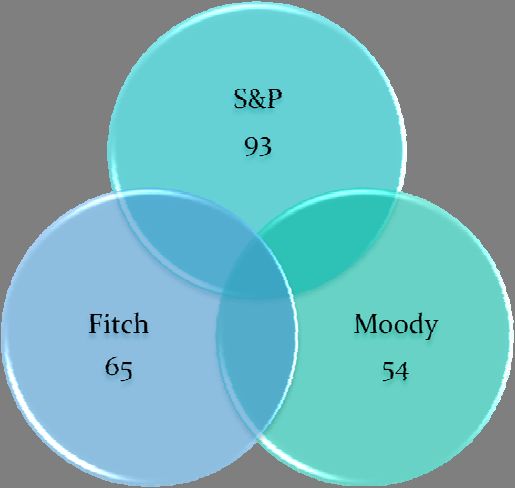
The differences in opinions between rating agencies can be represented in various ways.
In this paper we focus on rating changes as events. Below, we present a Venn diagram that
summarizes the distribution of events across the three rating agencies, and their overlap. As
explained, in the baseline each event has a 21-day window. Thus, an overlap (or a potential
agreement) occurs when rating changes for the different agencies happen within the same
window. For example, out of 141 events for S&P,12 21 overlap with events of Fitch, 12 with
events of Moody’s, and 15 with the two rating agencies concurrently. The general message that
emerges from Figure 2 is that the overlap is relatively small across the three rating agencies. This
suggests that the rating agencies do not always act concurrently, and hence that disagreements
between agencies persist. In turn, this suggests that the informational content of the events
across the agencies might be different. In particular, if the credit ratings are not perfectly
correlated then they all three cannot be fully explained by the exact same statistic (in this case,
the spread). In other words, given how uncorrelated the actions of the ratings agencies are, it
should be a priori clear that they provide different information among themselves. And if one of
these ratings is perfectly explained by the spread, then the other two can not. Therefore, in the
12
We use 141 events, rather than the total of 145 events in table 2, because there are 4 events that happen within the
window of a previous event. Thus, we drop these to avoid double counting when comparing with the other rating
agencies. We do the same for Moody’s and Fitch, where we drop 4 and 5 events respectively.
18analysis that follows, we consider these differences and test the validity of our results using the
data from the three rating agencies.
Figure 2. Venn Diagram
21 12
15
5
4. Results
4.1 Specification Test
We apply a standard Hausman specification test. This is performed in two steps. First we
estimate the following models:
OLS Model
y i ,t = α OLS × ii ,t + θ × VIX i ,t + κ i + ε i ,t ; i = events, and t =days
where yi ,t is, alternatively: ii ,t +1 (i.e., the spread one day forward); si ,t (i.e., the stock market
index); and neri ,t (i.e., the nominal exchange rate); κ i is an event-fixed effect, and ε i,t is the
error term. The VIX is included to control for the effect of global factors.
We also run instrumental-variables version of this regressions, where the only variant is
that we instrument spreads with ratings:
19IV-Model
y i ,t = α IV × ii ,t + θ × VIX i ,t + κ i + ε i ,t
ii ,t = ri ,jt
where j is, alternatively: S&P, Moody’s or Fitch ratings.
For robustness checks purposes, we also run an error-correction model for the case when
the dependent variable is the spread. In this case, the estimated equation is as follows:
Error-Correction Model
Δi = α × ii ,t + θ × VIX i ,t + φ × ΔVIX + κ i + ε i ,t
where Δi = ii ,t +1 − ii ,t , and ΔVIX = VIX i ,t +1 − VIX i ,t
In the IV-variant of the error correction model, we simply instrument the spread with the
rating.
The second step consists of applying a specification test using the estimates from these
models. Hausman (1978) proposes a test where a quadratic form in the differences between two
vectors of coefficients, scaled by the matrix of the difference in the variances of these vectors,
gives rise to a test statistic (chi-squared). Under the null hypothesis, OLS is consistent and
efficient, while IV is consistent but inefficient. On the other hand, under the alternative
hypothesis OLS is inconsistent, but IV continues to be consistent.
Table 4 summarizes the results we obtain when we apply this test to our baseline
specification (i.e., using all the events—upgrades and downgrades— from S&P, and a window
of 21-days per event).13 Every column in the table is a different dependent variable, and the last
column is the error-correction model. In the first two rows, we report αOLS and αIV, respectively.14
Thus, the coefficient reported in the first row under the first column is the OLS estimate for the
effect of the current spread on the spread one day forward.
The OLS results suggests that increases in the spread have a positive effect on the spread
forward (first and fourth columns), are related to decreases in the stock market index (second
13
For this purpose, we stack all the events (i.e., both upgrades and downgrades) together and run the regressions for
the full sample of S&P events.
14
We omit to report the coefficient for the VIX in the standard OLS and IV regressions, and the rest of the
coefficients in the error correction model, as they are not essential for explaining the test we perform in this section.
20column) and are also related to depreciations of the nominal exchange rate vis-à-vis the US
dollar (third column). The IV results (i.e., instrumenting spreads with ratings) are qualitatively
similar. What the Hausman specification test reveals is, in essence, if these coefficients are also
quantitatively the same.15 If they are statistically different, the null hypothesis is rejected—i.e.,
OLS is inconsistent. Quite importantly for our purposes, the rejection of the null hypothesis is
evidence that the spread is not a sufficient statistic.
In the next two rows of Table 4, we report the Hausman statistic (chi-squared) and the
corresponding p-value. The results are that the null hypothesis is rejected at standard confidence
levels (10 percent or less) in three out of four cases. This suggests that, for these selected macro
variables, the spread is not a sufficient statistic. In other words, not all the information in the
rating is reflected in the spread, and thus the rating explains some of the variation in these macro
variables. It is worth re-emphasizing here that the test is valid even if the OLS regression is mis-
specified, at least for the most common forms of misspecification.
The next step consists of checking the robustness of these results: we want to evaluate if
we get a high number of rejections for the specification test across different possible variants. In
Table 5 we summarize the results of a series of robustness checks. The first set of checks
consists of splitting the sample of events into upgrades and downgrades and running the
regressions separately. Next, we repeat the same exercise for both the full and the split samples,
using the events of Fitch and Moody’s. Then, we go back to the S&P data and change the event
window to 11 days per event (i.e., 5 days around the rating change), and also to 41 days per
event (i.e., 20 days around each rating change). Finally, we drop the few events that occur
within the same 21-day window (contemporaneous events).16
For each of these alternative specifications we run the OLS, IV and error correction
models, and perform the corresponding Hausman test. In table 5 we report the p-values. For
comparability purposes, in the first row we report the p-values from the previous regressions
(Table 4). The last row and the last column in the table are the “rejection rates,” i.e., the
percentage of rejections of the null hypothesis for each row or column.
15
This is not technically correct, as the Hausman procedure uses all the estimated coefficients, and their variance
matrix, to perform the test.
16
In the case of S&P, these are four events that happen within the window of a previous event.
21The results are very telling: the rejection rate varies between 56 and 75 percent in every
column, which means that we reject a lot across many possible permutations of the dependent
variable and also the estimation model. In the case of the rows, the rejection rate is below 50
percent only once: i.e., Fitch upgrades and downgrades. The high rejection rates across the board
reinforce the conclusion that the spreads are not a sufficient statistic. In other words, there seems
to be some informational content in ratings that is not captured by the spreads.17
At this point we can also evaluate the robustness of the test to the misspecifications that
we are not fully able to solve analytically. In particular, recall from the methodological section
that if the errors in the rating equation are also correlated with the fundamental (non-classical),
then the estimate of the IV is slightly different from the OLS. In this case, the estimates (IV and
OLS) will be different under the null hypothesis. If this form of misspecification is significant,
we expect more rejections the bigger the windows are. The reason is that the error in variables
implied in the rating grows with the window in which the rating is not changing. We do not find
this in our tests. On the contrary, if anything, focusing on the case of the full sample (upgrades
and downgrades for S&P) we find that the rejection rate is smaller when the width of the event
window is increased to 20 days around the event.18 Despite this, and even if we this particular
form of misspecification is significant and we do not find more rejections when we expand the
window simply because widening the window weakens the power of the test (because the
instrument becomes noisier, and hence weaker), the reader should rest assured that the validity of
the test is not invalidated because, as explained in Section 2, we still expect to find rejections if
the rating is providing information above and beyond the one contained in the spread. The only
difference is that we can not disentangle whether this information comes from the rating change
itself or from the noise.
17
We also run the same tests including a time trend in the regressions for each event window. We find somewhat
lower rejection rates, although in most cases they remain over 50%. It is hardly surprising that the rejection rates fall
when we include a time trend, as many events are anticipated (more on this below) and the effect of the anticipation
may be precisely a trend over the event window for the macro variables. Thus, we find it reassuring that we still find
a high number of rejections even when we include a trend.
18
We reject 3 out of 4 times when the window is 10 days around the event, and only 2 times when the window is
expanded.
22At the same time, if the rating is a non-linear function of the fundamental, then the non-
linearity can be interpreted as a non-classical EIV, which means that the larger the window, the
more severe the non-linearity and the higher the chance of rejecting the specification test. Thus,
some of the rejections that we obtain with larger windows might be spurious. Despite this
possibility, our results are also robust to defining the windows very tightly. The rejection rate for
the cases when the width of the event window is only five days around the event is 75 percent—
the same as the baseline—hence, indicating that the EIV introduced by the non-linearity is not
significantly large.
Having established that spreads and ratings are different, in the next section we run a
horse race between these variables. If ratings have informational content as we suggest, then we
expect that when we run a regression where both variables are included on the RHS, the rating
should be significant after controlling for the spread.
23Table 4. OLS vs. IV
Spread t+1 Stock Market Exchange Rate Spread t+1 (Error Correction)
OLS 0.906*** -0.217*** 0.100*** -0.095***
[0.010] [0.009] [0.007] [0.010]
IV 1.008*** -0.280*** 0.109*** 0.008
[0.025] [0.024] [0.017] [0.025]
Hausman Test (Ch^2) 20.13 8.03 0.33 20.48
P-value 0.001 0.018 0.848 0.001
S&P ratings are used for these regressions.
To perform these estimations the data is arranged to allow a 21-day window around the day of the change in the rating.
The OLS coefficient is the estimated effect of the change in spread on the corresponding dependent variable.
The IV is the coefficient obtained when the spread is instrumented by the rating.
All these regressions include event fixed effects and the Volatility Index (VIX) as controls.
The null hypothesis in the Hausman test is that the OLS estimator is more efficient.
24Table 5. Hausman Test, P-values
Spreadt+1 (Error Rejection
Spreadt+1 Stock Market Exchange Rate
Correction) rate1
Standard & Poor's (downgrades + upgrades) 0.001 0.018 0.848 0.001 75%
Standard & Poor's (downgrades) 0.010 0.800 0.436 0.018 50%
Standard & Poor's (upgrades) 0.001 0.140 0.001 0.015 75%
Fitch (downgrades + upgrades) 0.430 0.600 0.001 0.700 25%
Fitch (downgrades) 0.960 0.001 0.001 0.960 50%
Fitch (upgrades) 0.190 0.001 0.031 0.420 50%
Moodys (downgrades + upgrades) 0.066 0.061 0.082 0.160 75%
Moodys (downgrades) 0.355 0.053 0.001 0.725 50%
Moodys (upgrades) 0.078 0.009 0.001 0.154 75%
Standard & Poor's - 5 day window (all) 0.001 0.078 0.771 0.001 75%
Standard & Poor's - 5 day window (downgrades) 0.001 0.770 0.018 0.021 75%
Standard & Poor's - 5 day window (upgrades) 0.100 0.017 0.001 0.235 75%
Standard & Poor's - 20 day window (all) 0.001 0.660 0.850 0.001 50%
Standard & Poor's - 20 day window (downgrades) 0.001 0.001 0.670 0.001 75%
Standard & Poor's - 20 day window (upgrades) 0.001 0.068 0.001 0.001 100%
Standard & Poor's - Without contemporanous change in rating 0.000 0.091 0.953 0.002 75%
2
Rejection rate 75% 69% 63% 56%
1
Corresponds to number of rejections of the null hypothesis in the Hausman test over the total regressions run per dependent variable
2
Corresponds to number of rejections of the null hypothesis in the Hausman test over the total regressions run per specification
Every cell is the P-value of the Hausman test in the correspondent OLS versus IV regressions.
254.2 Horse Race
Having established that spreads are not a sufficient statistic, we turn now to estimating a new
model in which we exploit the informational content of ratings in order to explain the variation in
three macro variables using high frequency data.
We estimate the following OLS model:
y i ,t = α × ii ,t + β × ri ,jt + θ × VIX i ,t + κ i + ε i ,t ; i = events, and t =days
where yi ,t is, alternatively: ii ,t +1 ; s i ,t ; neri ,t ; κ i is an event-fixed effect, and ε i,t is the error
term. The VIX is included to control for the effect of global factors.
For robustness checks purposes, we also run an error-correction model for the case when
the dependent variable is it . In this case, the estimated equation is as follows:
Error-Correction Model
Δi = α × ii ,t + β × ri ,jt + θ × VIX i ,t + φ × ΔVIX + κ i + ε i ,t
where Δi = ii ,t +1 − ii ,t , and ΔVIX = VIX i ,t +1 − VIX i ,t
It is clear from the previous discussion on mis-specification that we cannot interpret the
magnitude of these coefficients in a structural way. Therefore, in what follows we just focus on
the signs and their statistical significance. We want to test if ratings explain part of the variation
in the cumulative returns of the macro variables over the selected event windows after we control
for spreads, and also if rating and spreads are correlated to these macro variables in ways that
make intuitive sense.
The results are reported in Table 6. The table is organized slightly different than the
previous ones. The panel on the upper LHS has the results for the baseline regressions: S&P, all
events, and a 21-day window for each event. Every row is a different regression: either a
different dependent variable or the error correction model. Every column is the estimated
coefficient for the corresponding RHS variable. The standard errors are reported in parenthesis
below every point estimate. In order to make the interpretation easier, we put asterisks next to
the coefficients that are statistically significant.19 Thus, the first row shows the results of
estimating the model by OLS for the case in which the dependent variable is the spread one day
19
*: significant at 10 percent, **: significant at five percent, and ***: significant at one percent.
26forward. We find that, as expected, α is positive and statistically significant, meaning that
increases in the spread today (i.e., a higher perceived probability of default) are correlated with
increases in the spread tomorrow.
Interestingly, β enters with a negative sign and is also statistically significant, meaning
that an increase in the rating (i.e., an upgrade) is correlated with a decrease in spreads one day
forward. The fact that the rating is significant after controlling for the spread is additional
evidence in favor of the hypothesis that spreads are not a sufficient statistic. The third RHS
variable included in the regression, the VIX, is positive but not statistically significant.
Next, we change the LHS variable to the stock market index. In this case we find that
increases in the spread are associated with decreases in the stock market indices, while an
increase in the rating, controlling for the spread, is correlated to a statistically significant increase
in the stock market. Finally, in this case, the coefficient estimate for the VIX is negative and
statistically significant.
The next row presents the results for the case in which the LHS variable is the nominal
exchange rate vis-à-vis the US dollar. The results are that increases in the spread are associated
to nominal exchange rate depreciations, a result that we find consistent with what we would
expect for emerging market economies: higher probability of default is oftentimes associated
withcapital flight and a weakening of the domestic currency. At the same time, the estimated
effect for changes in the rating, in this case, is not statistically significant. Note, incidentally, that
this is the one case for which we did not reject the Hausman test for the baseline specification in
Table 4. This is additional evidence in favor of the power of the test: in the case where we do
not reject the specification test, we find that the rating is insignificant after controlling for the
spread (i.e., the rating provides no additional information). Finally, we find that the coefficient
estimate for the VIX is also positive and statistically significant.
In the last row, we report the results of the error correction model.20 The results are
reassuringly similar to those in the first row, which are based on the same dependent variable.
The only difference is that the coefficient estimate for the VIX, while still positive, is now
statistically significant at the 10 percent level.
20
We omit the coefficient estimates for φ , as they are not essential.
27Next, we rerun the baseline specification splitting the sample between upgrades and
downgrades. The results for the case of downgrades are reported in the upper-center panel, while
for the downgrades are reported in the upper-right panel. The results are very similar to the
previous ones, with only a couple of differences. When we focus on downgrades, we find that
the estimated effect of changes in the rating is no longer statistically significant when the LHS
variable is the stock market. In the case of upgrades, the coefficient estimate for the effect of
changes in rating on the nominal exchange rate is now positive and significant.
The middle panels of Table 6 report the results for the same exercise, but for the case of
the events from the other two rating agencies. For concreteness, we concentrate only on the cases
of the full sample (upgrades and downgrades stacked together). We find that in all cases, the
coefficient estimate for α enters the regressions with the expected sign and is statistically
significant: increases in the spread today are associated with higher spreads tomorrow, decreases
in the stock market, and nominal exchange rate depreciations. In the case of β, the estimated
effect of changes in the rating, we find that for Fitch events, they typically have no explanatory
power, except in the case when the macro variable is the exchange rate: in that case, we find that
increases in the ratings (i.e., upgrades) are associated with nominal appreciations. This is
interesting because this is the one case where we find an insignificant estimate for S&P. Also, it
is consistent with the results of the specification test: in the case of Fitch, full sample, we reject
the null hypothesis only when the dependent variable is the nominal exchange rate. Instead, in
the case of Moody’s, the rating always enters the regressions with the expected sign and is
statistically significant: upgrades are associated with decreases in the spread forward, increases
in the stock market, and nominal appreciations. In the case of the VIX, the coefficient estimates
are always significant in both samples and have the same signs: increases in the VIX are
associated with higher spreads forward, lower stock market indices, and more depreciated
nominal exchange rates.
Finally, in the lower panels of Table 6 we report the results for the cases in which we
narrow the width of the event window to five days around the event and, alternatively, expand it
to 20 days. We report the results based on the S&P sample only (upgrades and downgrades). The
results are reassuringly similar to those of the baseline specification, with one exception. For the
case of the expanded window, the effect of rating changes on the stock market is not statistically
significant.
28In summary, there are a few important takeaways from this section. First, the results from
the horse race exercise suggest that ratings usually enter these regressions with a statistically
significant sign after controlling for the spread. In the case of S&P ratings, this is true in three
out of the four regressions; in the case of Moody’s sample, it is always true; and in the case of
Fitch ratings, it is true in just one case (which is incidentally the case when it is not true for
S&P). This is consistent with the results from the specification tests (i.e., we reject less for
Fitch). At the same time, the high rate of rejections across the board suggests that spreads are not
a sufficient statistic for the rating. Second, the additional robustness checks show that these
results are consistent when we split the sample between upgrades and downgrades, and also to
expanding and narrowing the event window.
29Table 6. OLS with Event Fixed Effects
S&P upgrades & downgrades S&P downgrades S&P upgrades
Spread Rating VIX Spread Rating VIX Spread Rating VIX
Spreadt+1 0.884*** -0.006*** 0.006 0.894*** -0.006*** 0.013 0.876*** -0.007*** -0.003
[0.011] [0.0014] [0.015] [0.014] [0.001] [0.017] [0.017] [0.001] [0.022]
Stock Market -0.205*** 0.004*** -0.104*** -0.484*** -0.002 -0.067*** -0.018** 0.002** -0.085***
[0.011] [0.014] [0.001] [0.020] [0.002] [0.025] [0.008] [0.001] [0.012]
Exchange Rate 0.098*** -0.0005 0.045*** 0.196*** -0.003 0.089*** 0.007** 0.002*** -0.006
[0.008] [0.0009] [0.010] [0.018] [0.002] [0.022] [0.003] [0.0003] [0.005]
Δ Spread -0.117*** -0.006*** 0.029* -0.109*** -0.006*** 0.030* -0.124*** -0.006*** 0.027
[0.011] [0.001] [0.015] [0.014] [0.001] [0.018] [0.017] [0.0019] [0.024]
Fitch upgrades and downgrades Moodys upgrades & downgrades
Spread Rating VIX Spread Rating VIX
Spreadt+1 0.863*** -0.002 0.036*** 0.855*** -0.004** 0.040***
[0.010] [0.001] [0.011] [0.013] [0.002] [0.015]
Stock Market -0.404*** 0.002 -0.132*** -0.297*** 0.005** -0.140***
[0.016] [0.002] [0.017] [0.014] [0.002] [0.016]
Exchange Rate 0.225*** -0.009*** 0.033** 0.190*** -0.003** 0.046***
[0.013] [0.002] [0.014] [0.010] [0.0014] [0.012]
Δ Spread -0.139*** -0.001 0.064*** -0.147*** -0.004** 0.070***
[0.010] [0.001] [0.012] [0.013] [0.002] [0.015]
S&P 5 day window S&P 20 day window
Spread Rating VIX Spread Rating VIX
Spreadt+1 0.742*** -0.005*** 0.013 0.941*** -0.005*** 0.021***
[0.019] [0.001] [0.019] [0.006] [0.0009] [0.007]
Stock Market -0.234*** 0.003** -0.040** -0.271*** 0.001 -0.173***
[0.018] [0.001] [0.017] [0.009] [0.002] [0.011]
Exchange Rate 0.048*** -0.0007 0.026* 0.168*** -0.0006 0.093***
[0.013] [0.001] [0.013] [0.007] [0.001] [0.009]
Δ Spread -0.257*** -0.005*** 0.029 -0.060*** -0.005*** 0.037***
[0.019] [0.001] [0.021] [0.006] [0.0009] [0.008]
These regressions include event fixed effects as controls.
30You can also read