DUT: Learning Video Stabilization by Simply Watching Unstable Videos

DUT: Learning Video Stabilization by Simply Watching Unstable Videos

 Yufei Xu1 Jing Zhang1 Stephen J. Maybank2 Dacheng Tao1
 1
 UBTECH Sydney AI Centre, Faculty of Engineering, The University of Sydney
 2
 Department of Computer Science and Information Systems, Birkbeck College
arXiv:2011.14574v2 [cs.CV] 1 Dec 2020

 Supervised Learning

 Trajectory Smoother

 Unstable Video Unstable Video Stabilized Video Paired Stable Video
 (a) Traditional stabilization methods (b) DNN-based stabilizers
 Unsupervised Learning

 Trajectory Smoothing

 Unstable Video Unstable Input Stabilized Output Traditional DNN-based DUT
 Content Consistency
 (c) Our DUT with deep learning and trajectory estimation (d) Stabilization results

 Figure 1. Comparison of our DUT and other stabilizers. (a) Traditional methods estimate the trajectory using hand-crafted features and
 smooth it with a fixed-kernel smoother. Stabilized frames are warped from the unstable one (marked in transparent color) according to the
 smoothed trajectory. (b) DNN-based methods directly generate the stabilized results without explicitly modeling the smoothing process.
 The pipeline is hard to control and may produce distortion. (c) Our DUT stabilizes videos with explicit trajectory estimation and smoothing
 using DNNs. (d) Stabilized results of a traditional method [15] (over-crop and shear), DNN-based method [29] (distortion), and DUT.

 Abstract 1. Introduction

 We propose a Deep Unsupervised Trajectory-based sta- Videos captured by amateurs using hand-held cameras
 bilization framework (DUT) in this paper1 . Traditional sta- are usually shaky, leading to unpleasing visual experiences.
 bilizers focus on trajectory-based smoothing, which is con- Moreover, unstable videos also increase the complexity of
 trollable but fragile in occluded and textureless cases re- subsequent vision tasks, such as object tracking and visual
 garding the usage of hand-crafted features. On the other simultaneous localization and mapping (SLAM). Video sta-
 hand, previous deep video stabilizers directly generate sta- bilization is to remove the undesirable shake and generate
 ble videos in a supervised manner without explicit trajec- a stabilized video from the unstable one, thereby improving
 tory estimation, which is robust but less controllable and the visual experience and facilitating down-stream tasks.
 the appropriate paired data are hard to obtain. To con- Traditional video stabilization methods [14, 15, 16, 17,
 struct a controllable and robust stabilizer, DUT makes the 18, 19, 32] usually adopt a trajectory-based pipeline con-
 first attempt to stabilize unstable videos by explicitly esti- sisting of three components: 1) keypoint detection, 2) tra-
 mating and smoothing trajectories in an unsupervised deep jectory estimation based on keypoint tracking, and 3) tra-
 learning manner, which is composed of a DNN-based key- jectory smoothing, as illustrated in Figure 1(a). Once the
 point detector and motion estimator to generate grid-based smoothed trajectory is obtained, the stabilized video can be
 trajectories, and a DNN-based trajectory smoother to sta- generated by warping the unstable one. However, several
 bilize videos. We exploit both the nature of continuity in challenges degrade these methods. First, the keypoint de-
 motion and the consistency of keypoints and grid vertices tector is usually based on hand-crafted features, which are
 before and after stabilization for unsupervised training. Ex- less discriminative and representative in textureless and oc-
 periment results on public benchmarks show that DUT out- cluded areas. Second, the keypoint tracker such as the KLT
 performs representative state-of-the-art methods both qual- tracker may fail when there is a large appearance variance
 itatively and quantitatively. around keypoints due to occlusion, illumination, viewpoint
 change, and motion blur as shown in Figure 1(d). Third, a
 1 Our code is available at https://github.com/Annbless/DUTCode. smoother with a fixed kernel is always used for trajectory

 1

smoothing, which cannot adapt to various trajectories with as 2D motion on the image plane [30, 5]. A typical way
different long- and short-term dynamics. is to detect and track keypoints across all the frames and
 Recently, some deep learning-based methods have been obtain the smoothed temporal trajectory via optimization,
proposed [3, 8, 29, 31, 33, 34, 37]. Unlike the tradi- such as low-rank approximation [15], L1 norm optimiza-
tional trajectory-based methods, they prefer to regress the tion [7], bundled optimization [18], epipolar geometry [6],
unstable-to-stable transformation or generate the stabilized and geodesics optimization[36]. These methods need long-
video directly in an end-to-end manner as illustrated in Fig- term tracked keypoints to estimate complete trajectories,
ure 1(b). Although they can stabilize videos well, several which is challenging due to the appearance variance around
issues exist here. First, these methods are less controllable keypoints. Recently, motion profile (Mp)-based methods
and explainable, making it hard to diagnose and improve have attracted increasing attentions [16, 19]. Mp describes
the network components when there are large unexpected frame-to-frame 2D motions at specific locations, e.g., dense
distortion or over-crop [29], e.g., in complex scenes with pixels or sparse vertices from predefined grids, and obtains
multiple planar motions as shown in Figure 1(d). Second, the trajectories by associating corresponding pixels or ver-
training deep models requires large-scale unstable and sta- tices across all the frames. Although the Mp-based stabi-
ble video pairs, which are hard to collect in the real world. lization pipeline is simple and effective, it may fail in oc-
Although some methods [3, 34] propose to use pseudo un- cluded and textureless areas due to the limited ability of
stable videos, they dismiss the depth variance and dynamic hand-crafted features. We also adopt the Mp-based tra-
objects in real scenes, thereby introducing a domain gap and jectory description but revolutionize the key modules with
impairing the model’s generalization ability. novel neural ones, which can handle challenging cases by
 To address the aforementioned issues, we make the first leveraging the powerful representation capacity of DNNs.
attempt to stabilize unstable videos by explicitly estimat- 3D Methods. 3D methods estimate and smooth cam-
ing and smoothing trajectories using unsupervised DNN era paths in 3D space and construct point clouds for pre-
models as illustrated in Figure 1(c). Specifically, a novel cise construction and re-projection [35, 9]. For example,
Deep Unsupervised Trajectory-based stabilizer (DUT) is Liu et al. leverage structure from motion (SfM) [27] to con-
proposed, including three neural network modules: key- struct 3D camera paths and use content preserving warp-
point detection (KD), motion propagation (MP), and trajec- ing to synthesize stabilized frames in [14]. Although this
tory smoothing (TS). First, the KD module detects distinct pipeline is appealing since it can describe the exact 3D cam-
keypoints from unstable image sequences along with their era motion, SfM itself is a challenging task that estimating
motion vectors calculated by an optical flow network. Next, accurate camera poses and 3D point clouds is difficult when
the MP network propagates the keypoints’ motion to grid there are large occlusions, heavy blur, and dynamic objects.
vertices on each frame and obtain their trajectories by as- Recently, special hardware is used [17, 23, 11] for precise
sociating corresponding vertices temporally, which are then camera pose estimation and 3D reconstruction from regular
smoothed by the TS module. The stabilizer is optimized videos or 360◦ videos [26, 12]. However, the need for auxil-
to estimate the trajectory by exploiting the nature of con- iary hardware limits their usage scenarios. Although we use
tinuity in motion and smooth the trajectory by keeping the Mp to describe 2D trajectory rather than 3D camera path, it
consistency of keypoints and vertices before and after stabi- indeed follows the “divide-and-conquer” idea by using local
lization, leading to an unsupervised learning scheme. 2D planar transformation in each grid as an approximation
 The main contributions of this paper are threefold: of the 3D transformation, which is effective in most cases.
 • We propose a novel DUT stabilizer that firstly esti-
mates and smooths trajectories using DNNs, which is more DNN-based Methods. Recently, DNN-based video sta-
effective than traditional counterparts to handle challenging bilizers have been proposed to directly regress unstable-to-
cases owing to its powerful representation capacity while stable transformation from data. Wang et al. uses a two
inheriting the controllable and explainable ability. branch Siamese network to regress grid-based homography
 • We propose an unsupervised training scheme for stabi- [29]. Xu et al. leverage several spatial transformer net-
lization that does not need paired unstable and stable data. works (STN) [10] in the encoder to predict the homography
 • DUT outperforms state-of-the-art methods both quali- gradually [31]. Huang et al. exploit multi-scale features
tatively and quantitatively on public benchmarks while be- to regress global affine transformation [8]. Although they
ing light-weight and computationally efficient. can obtain stabilized videos, it is difficult for them to adapt
 to background depth variance and dynamic foreground ob-
2. Related Work jects, thereby producing distortion in these cases. Recently,
 Yu et al. leverage a convolutional neural network (CNN)
 We briefly review representative traditional (2D and 3D) as an optimizer and obtain stabilized video via iteratively
methods and DNN-based stabilizers as follows. training [33], which is computationally inefficient. Choi et
 2D Methods. 2D methods describe the camera path al. proposes a neighboring frame interpolation method [3],

 2

Smoothed Trajectories

 Iterative smoother
 Optical Flow Sparse Keypoints motion Dense Grid motion Unstable trajectory Smooth trajectory

 Keypoint Detection Motion Propagation Trajectory Smoothing Stabilized
 Module Module Module Frames Sigmoid

 RGB Frames Kernel Scale
 (a) Pipeline Decoder Decoder

 T-Block

 Distance Encoder D-Block W-Block
 Trajectory Encoder

 Motion
 Decoder

 Sparse Keypoints motion C Dense Grid Motion
 Unstable Trajectories
 Motion Encoder M-Block DM-Block
 (b) Motion Propagation Module (c) Trajectory Smoothing Module

 1D Conv LeakyReLU SoftMax 3D Conv ReLU C Concat Element-wise Multiply Sum

Figure 2. (a) The pipeline of our video stabilization framework, which contains three modules: keypoint detection module, motion prop-
agation module, and trajectory smoothing module. The keypoint detection module utilizes the detector from RFNet [22] and optical flow
from PWCNet [25] for motion estimation. (b) The motion propagation module aims to propagate the motions from sparse keypoints to
dense grid vertices. It employs two separate branches of stacked 1d convolutions to embed keypoint location and motion features, generate
attention vector and attended features to predict the motion vector for each grid vertex. (c) The trajectory smoothing module aims to
smooth the estimated trajectories at all grid vertices by predicting smoothing kernel weights. Three 3d convolutions are stacked to process
the trajectories both spatially and temporally. The estimated kernel and scale are multiplied to form the final kernel for iterative smoothing.

which can generate stable videos but may also introduce keypoint detectors [2, 20, 28] and other deep learning-based
ghost artifacts around dynamic objects. Yu et al. introduces ones [4, 21], RFNet can efficiently produce high-resolution
a two-stage method [34] that uses optical flow based warp- response maps for selecting robust keypoints since it adopts
ing for stabilization while requiring the pre-stabilization re- a multi-scale and shallow network structure.
sult by a traditional method. Denote the input video as {fi |∀i ∈ [1, E]}, where fi
 By contrast, our DUT method stabilizes unstable videos is the ith frame of the video and E is the number of
by explicitly estimating and smoothing trajectories using frames. The detected keypoints can be expressed as {pij =
DNN models. It inherits the controllable and explainable KD (fi ) |∀i ∈ [1, E], ∀j ∈ [1, L]}, pij is the jth detected
ability from trajectory-based stabilizers while being effec- keypoint on frame fi , KD (·) denotes the keypoint detector
tive to handle challenging cases owing to the powerful rep- embodied by RFNet, L is the number of detected keypoints,
resentation capacity. Moreover, it does not require paired which is set to 512 in this paper. For simplicity, we use the
data for training. same symbol pij to denote the keypoint location without
 causing ambiguity. Once we obtain the keypoints, we can
3. Methods calculate their motion vectors from the optical flow field.
 In this paper, we adopt PWCNet [25] to calculate the opti-
 As shown in Figure 2, given an unstable video as input, cal flow. We denote the keypoints and their motion vector
DUT aims to generate a stabilized video. It consists of three as {(pij , mij )|∀i ∈ [1, E − 1], ∀j ∈ [1, L]}, where mij de-
key modules: 1) keypoint detection, 2) motion propagation, notes the motion vector of the keypoint pij on frame fi .
and 3) trajectory smoothing, which are detailed as follows.
 3.2. Motion Propagation (MP)
3.1. Keypoint Detection (KD)
 3.2.1 CNN-based Motion Propagation
 The keypoint detection module aims to detect keypoints
and calculate their motion vectors, which is the preliminary Since there are always multiple planar motions existing in
step to construct the motion profile. In this paper, we adopt the real-world unstable videos due to background depth
the RFNet [22] as our keypoint detector, which is trained variance and dynamic foreground objects, using a single
on the HPatchs dataset [1]. Compared with the traditional global homograph to model the frame-to-frame transforma-

 3

tion or unstable-to-stable transformation is inaccurate. To k = 1, . . . , M N , the motion propagation module predicts
address this issue, we adopt the grid-based motion profiles the residual motion vector ∆nik for each vertex vik , i.e.
to describe the motions. Specifically, each frame is uni-
 ∆nik = M P ({(∆mij , dijk ) |∀j ∈ [1, L]}) , (2)
formly divided into a fixed set of grids, i.e., M×N grids in
this paper. The local motion within each grid is treated as a where M P (·) denotes the proposed MP network. The dis-
planar motion, which is reasonable. It can be described by a tance vectors and motion vectors of size [M N, L, 2] (after
frame-to-frame homograph transformation derived from the tiling) are fed into two separate encoders as shown in Fig-
motion vectors of grid vertices. However, we only have the ure 2(b). The encoded features are further embedded by
motion vectors of keypoints distributed in these local grids. several 1D convolutions. Then, the attention vector of size
How to propagate the motion vectors to each grid vertex is [M N, L, 1] is obtained based on the distance embeddings
challenging. In contrast to existing methods, which use a and used to aggregate the features from concatenated mo-
median filter to estimate the motion vector of each vertex tion embeddings and distance embeddings, generating the
from its neighboring keypoints, we devise a novel motion attended feature of size [M N, 1, 2], which is further used
propagation module based on DNNs by exploiting the na- to predict the final dense residual motions ∆nik through a
ture of continuity in motion, which can obtain more robust motion decoder. Details of the MP network can be found
and accurate motion vectors for each grid. in the supplementary material. Then we can calculate the
 target motion vector nik of each vertex vik as follows by
 referring to Eq. (1),
 nik = ∆nik + (Hic (vik ) − vik ) , (3)
 Note that we reuse the same symbol vik to denote the grid
 vertex location for simplicity like pij . Besides, we choose
 (a) (b) (c)
 Hic for each vertex vik according to the majority cluster in-
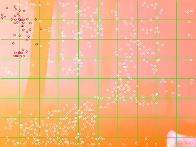
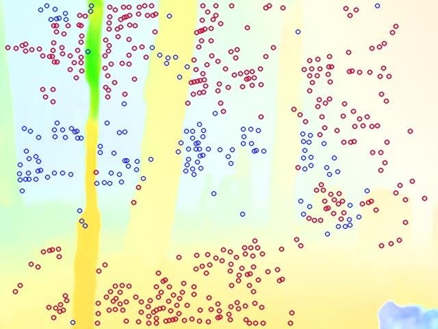
Figure 3. (a) An input image. (b) Inliers (red points) and out-
 dex of its neighboring keypints in Ωik , which is defined as
liers (blue points) identified using the single-homography estima-
 Ωik = {j| kdijk k2 ≤ R}. Here, R is a predefined radius,
tion with RANSAC. (c) Two clusters of keypoints identified by
our multi-homography estimation method based on K-means. The i.e., 200 pixels in this paper. Unlike [16], which only uses
background of (b) and (c) is the visualized optical flow field of (a). a median filter to obtain the residual motion of each ver-
 tex from its neighboring keypoints’ residual motion vectors,
 Specifically, we adopt the idea in [16] by propagating the i.e., ∆nik = M edianF ilter ({∆mij |∀j ∈ Ωik }), the pro-
residual motion vectors. In [16], they use a global homog- posed neural network can model the characteristics of all
raphy transformation to calculate the reference motion vec- keypoint residual motion vectors and learn representative
tor of each keypoint and then calculate the residual. How- features to eliminate noise and predict accurate target resid-
ever, there may be multiple planar motions as shown in Fig- ual motion vectors, thereby outperforming the median filter
ure 3(b), thereby estimating a single homography leads to by a large margin as demonstrated in the experiments.
shear artifacts and large residuals. In this paper, we propose
a multi-homography estimation method to calculate more 3.2.2 Objective Function
suitable residuals with lower amplitudes, thereby facilitat- For the estimation of target motion vector nik of each vertex
ing the subsequent motion propagation process. vik , there are two constraints on it based on the assumption
 As shown in Figure 3(c), we first employ K-means [13] of local motion continuity. First, nik should be close to the
on {mij } to divide the keypoints on fi into two clusters, motion vectors of vik ’s neighboring keypoints. Second, the
i.e., Cic = {(pij , mij ) |∀j ∈ Λci }, where c = 0 or 1 denotes target position for each keypoint pij can be calculated based
the cluster index and Λci is the keypoint index set belonging on its motion vector mij or its projection by the homo-
to the cluster Cic . Note that when the number of keypoints grpahy transformation of the grid that contains pij , which
in any cluster is less than a threshold, i.e., 20%×L = 102 can be derived from the four grid vertices’ motion vectors
in this paper, we merge it into the master cluster. Then, we [16, 24]. Based on the above two constraints, we formulate
can estimate the global homography transformation for each the objective function for the MP module as:
cluster, denoting Hic . The residual motion vector ∆mij of
 E−1
 XM N
each keypoint can be formulated as: X X
 Lvm = λm knik − mij k1
 ∆mij = pij + mij − Hic (pij ) , ∀j ∈ Λci . (1) i=1 k=1 j∈Ωik
 E−1
 XX L
 2
Given ∆mij and the distance vector dijk between each + λv k pij + mij − Hij (pij ) k2 , (4)
grid vertex vik and keypoint pij , i.e., dijk = pij − vik , i=1 j=1

 4

where k·k1 denotes the L1 norm, k·k2 denotes the L2 norm, shown in Figure 2(c), the trajectory of size [2, E, M, N ]
Hij is the homography of the grid containing pij , λm/v is goes through the trajectory encoder with a 1×1 convolu-
the weight to balance the two terms. If λv = 0, the objective tion layer. The encoded feature of size [64, E, M, N ] is fed
function indeed leads to a median filter solution. In addition into several 3D convolution layers for further embedding,
to the keypoints-related contraints in Eq. (4), we also intro- which then goes through a kernel decoder and a scale de-
duce a shape preserving loss Lsp on each grid gim , i.e., coder in parallel, generating features of size [12, E, M, N ].
 The scale decoder output imitates the parameter λ in Eq. (8)
 X (M −1)(N
 E−1 X −1)
Lsp = 3
 vbim 2
 − vbim 1
 + R90 vbim 2
 − vbim
 

 2
 , while the kernel decoder generates smoothing kernels for
 2
 i=1 m=1 each vertex. To keep consistent with Eq. (8), the neighbor-
 (5) hood radius is 3. Thereby, there are 12 weights for each
 o o
where vbim = vim + noim , o = 1, 2, 3, 4, vim
 1 4
 ∼ vim denote vertex since we generate different weights for different di-
four vertices of gim in the clockwise direction, their mo- mensions. The generated weights are used for smoothing
tion vectors are n1im ∼ n4im , R90 (·) denotes rotation 90◦ the trajectory according to Eq. (8).
of a vector. Lsp accounts for spatial smoothness and avoids
large distortion in textureless regions. The final objective is: 3.3.3 Objective Function
 LM P = Lvm + λs Lsp , (6) To supervise the training of the CNN smoother, we devise
 an objective function by considering both spatial and tem-
where λs is loss weight that balances the two losses.
 poral smoothness as well as a content preserving loss, i.e.,
3.3. Trajectory Smoothing (TS) LT S = Lts + λs Lsp + λc Lcp , (9)
3.3.1 Jacobi Solver-based Smoother where Lts is same as defined in Eq. (7), Lsp is the spa-
Associating the motion vectors of corresponding grid ver- tial shape preserving loss similar to the one used for MP in
tices onPeach frame formulates the trajectories, i.e., Tk = Eq. (5) where the target position of vik after smoothing is:
 i
{tik = m=1 nmk |∀i ∈ [1, E]} [19, 16]. A typical way to vbik = vik + Tbik − Tik . (10)
smooth the trajectory is using the Jacobi Solver [19, 16, 18].
The smoothed trajectory should be locally smooth but close Moreover, since distortion in structural areas around key-
to the unstable one, which can be obtained by minimizing points affects the visual experience more than those in tex-
the following temporal smoothness loss Lts : tureless areas, we introduce a content preserving loss Lcp :
 E−1 L
 E−1 XX 2
 X 2 X 2 Lcp = k Bili(pij ) − Hij (pij ) k , (11)
 Lts = ik − Tik k2 + λ
 (kTc wij kTc
 ik − Tjk k2 ), (7)
 d
 i=1 j=1
 i=1 j∈Ωi
 where Hij is same as in Eq. (4). Assuming pij is in the
where Tc ik denotes the smoothed trajectory at vik , wij is the grid gim , then Bili (·) denotes a bilinear interpolation, i.e.,
 P4
weight controlling the local smoothness of the trajectory, λ Bili(pij ) = o=1 wo vbim o 1
 . Here, vbim ∼ vbim4
 are the tar-
balances the first data term and the second smoothness term, get positions of four vertices in gim after smoothing and
Ωi is the temporal neighborhood of fi , i.e., Ωi = [i−3, i+3] calculated as Eq. (10). w1 ∼ w4 are the interpolation co-
in this paper. Eq. (7) is a quadratic optimization problem efficients calculated based on the position of pij relative to
that can be solved by applying the Jacobi Solver iteratively: the four vertices of gim before smoothing, i.e., vim1
 ∼ vim4
 .
 P t−1 Lcp indeed preserves the shape of each grid containing key-
 t Tik + λ j∈Ωi wij T
 djk points, which probably has structural content. Note that the
 Tc
 ik = P , (8)
 1+λ j∈Ωi wij proposed CNN smoother can be trained using only unstable
 videos based on the objective in Eq. (9). In conclusion, the
where t denotes the number of iterations. However, the ker- stabilization process can be summarized in Algorithm 1.
nel weight wij of the Jacobi Solver is fixed regardless of the
local temporal dynamics of the trajectory. Besides, there are 4. Experiments
no spatial constraints on the trajectory in Eq (7), which may
result in distortion in the final stabilized video. We evaluated our model on public benchmark dataset
 NUS [18] and compared it with state-of-the-art video
 stabilization methods, including deep learning-based
3.3.2 CNN-based Smoother
 method [29, 3] and traditional methods [15, 16]. Both quan-
To address the above issues, we propose a novel CNN- titative and qualitative results as well as model complexity
based smoother that can generate dynamic smoothing ker- are provided for comprehensive comparison. Ablation stud-
nels based on the characteristics of the trajectories. As ies of key modules in our model were also conducted.

 5

Table 2. Distortion scores of different methods.
 Algorithm 1: Deep Unsupervised Trajectory-based Regular Parallax Running QuickRot Crowd Avg.
 Video Stabilizer (DUT) Meshflow 0.898 0.716 0.764 0.763 0.756 0.779
 Input: Unstable video: {fi |i ∈ [1, E]} SubSpace 0.973 0.855 0.939 \ 0.831 0.900
 Optical flow: {OFi |i ∈ [1, E − 1]}; DIFRINT 0.934 0.921 0.873 0.633 0.905 0.853
 Output: Stabilized video: {fbi |i ∈ [1, E]} StabNet 0.702 0.573 0.753 0.574 0.759 0.672
 Grid motion:{nik |i ∈ [1, E − 1], k ∈ [1, M N ]} DUT 0.982 0.949 0.927 0.935 0.955 0.949
 Estimated trajectory: {Tk |k ∈ [1, M N ]}
 Smoothed trajectory: {Tbk |k ∈ [1, M N ]};
 for i = 1 : E − 1 do Table 3. Cropping ratios of different methods.
 {pij |j ∈ [1, L]} = RF N et (fi ); ∀j,mij =OFi (pij ); Regular Parallax Running QuickRot Crowd Avg.
 if There are multiple planes in frame fi then
 Meshflow 0.686 0.540 0.584 0.376 0.552 0.548
 Hic = M ultiHomo ({pij |∀j}, {mij |∀j});
 else SubSpace 0.712 0.617 0.686 \ 0.543 0.639
 Hic = SingleHomo ({pij |∀j}, {mij |∀j}); DIFRINT 0.922 0.903 0.869 0.732 0.882 0.862
 end StabNet 0.537 0.503 0.512 0.418 0.497 0.493
 ∆mij = pij + mij − Hic (pij ) , ∀j ∈ Λci ; DUT 0.736 0.709 0.690 0.673 0.710 0.704
 for k = 1 : M N do
 dijk = pij − vik , ∀j ∈ [1, L];
 ∆nik = M P ({(∆mij , dijk ) |∀j ∈ [1, L]}); We compared our method with representative state-of-
 nik = ∆nik + (Hic (vik ) − vik ); the-art video stabilization methods, including traditional
 end methods: Subspace [15], Meshflow [16], and deep learning
 end methods: DIFRINT [3] and StabNet [29]. The quantitative
 for k = 1 : M N do results are summarized in Table 1. There are several empir-
 Tk = E−1 ical findings. Firstly, the proposed DUT stabilizer achieves
 P
 i=1 nik ; Tk = Smoother (Tk );
 c
 end better performance in challenging cases with multiple pla-
 for i = 0 : E do   nar motions, e.g., in the category of Parallax. Compared
 fˆi = Reprojection fi , {Tk |∀k}, {T ck |∀k} with Meshflow [16], DUT has less distortion indicated by
 end the distortion metric, owing to the introduction of multi-
 homography estimation. Secondly, the deep learning-based
 keypoint detector empowers DUT with better capacity in
 dealing with challenging cases compared with other tradi-
4.1. Experiment Settings tional stabilizers. In the category of Quick Rotation, which
 Unstable videos from DeepStab [29] were used for train- contains blur and large motion in the scenes, DUT still ob-
ing. Five categories of unstable videos from [18] were used tains a large margin over other stabilizers regarding dis-
as the test set. The metrics introduced in [18] were used for tortion and stability metrics. Subspace [15] even fails for
quantitative evaluation, including cropping ratio, distortion, videos in this category since it is difficult to track long-term
and stability. Cropping ratio measures the ratio of remain- robust keypoints. Thirdly, compared with StabNet [29],
ing area and distortion measures the distortion level after DUT produces less distortion and keeps more areas after
stabilization. Stability measures how stable a video is by cropping. Although StabNet also uses grid-based warp-
frequency domain analysis. All the metrics are in the range ing while being trained with paired data from the deepStab
of [0, 1]. A larger value denotes a better performance. More dataset, it does not achieve a balance between stability and
implementation details, user study results, and robustness distortion. By contrast, DUT simply uses unstable videos
evaluation can be found in the supplementary material. for training. As there are many possible stabilized videos
 that all look stable about the same, training with paired data
4.2. Quantitative Results that only provides one single stable instance for each sam-
 ple may be biased. Besides, the supervisory signal from
 Table 1. Stability scores of different methods. the stable video is less effective than those from the grid-
 Regular Parallax Running QuickRot Crowd Avg. based pipeline, which have explicit relationships to stabil-
Meshflow 0.843 0.793 0.839 0.801 0.774 0.810 ity, e.g., displacement derived from the grid motion and tra-
SubSpace 0.837 0.760 0.829 \ 0.730 0.789 ∗ jectory. Fourthly, compared with the interpolation-based
DIFRINT 0.838 0.808 0.822 0.835 0.791 0.819 DIFRINT [3], DUT produces less distortion around the dy-
StabNet 0.838 0.769 0.818 0.785 0.741 0.790 namic objects since it can handle them via robust keypoint-
DUT 0.843 0.813 0.841 0.877 0.792 0.833 based local grid warping. Generally, DUT achieves the best
∗
 The average score is not accurate since SubSpace fails to sta- performance regarding stability and distortion, which con-
bilize some of the videos in the category of Quick Rotation. firms the superiority of our trajectory-based DNN stabilizer.

 6

Input Video SubSpace MeshFlow DIFRINT Our DUT

Figure 4. Visual comparison between our DUT and SubSpace [15], Meshflow [16], DIFRINT [3]. We present five kinds of videos for
subjective evaluation, i.e., 1) moderate camera shake , 2) large dynamic objects, 3) small dynamic objects, 4) multiple planar motions,
and 5) quick camera rotation and blur in the first row to the fifth row, respectively. It can be observed that our method can handle diverse
scenarios compared with traditional stabilizers and deep learning-based methods. More results can be found in the supplementary video.

4.3. Subjective Results 4.4. Ablation Studies
 Some visual results of different methods are shown in 4.4.1 Motion Propagation Module
Figure 4. For videos containing dynamic objects (the 1st- Since the motion propagation module is crucial for the tra-
3rd rows), DIFRINT [3] is prone to produce ghost artifacts jectory smoother by providing accurate grid motions, we
around dynamic objects due to the neighboring frame inter- compared our MP network with traditional median filter
polation, which is unaware of dynamic foregrounds. Sub- (MF)-based method. Since we did not have ground truth
space [15] may generate some distortion if the dynamic ob- grid motion, we warped the future frame from the current
ject is large as in the 2nd row. For scenes containing par- frame based on the estimated grid motions and carried out
allax and occlusion (the 4th row), Subspace also produces the evaluation based on the warped frame and ground truth
distortion due to the inaccurate feature trajectory. DIFRINT frame. Specifically, we calculated the homography between
generates hollows since the interpolation cannot hallucinate them and used two metrics related to it for evaluation. First,
the occluded objects. Meshflow [16] produces shear arti- if the grid motion is accurate, the warped frame should be
facts due to the inaccurate homography estimated from a close to the ground truth frame, i.e., an identity homogra-
single plane. DUT has no such drawbacks since it adopts an phy. We calculated the Frobenius Norm of the difference
adaptive multi-homography estimation method. For videos between the estimated homography and the identity matrix
containing quick camera rotation and large blur (the 5th as the first metric: distance. Second, following [18], we cal-
row), Subspace and Meshflow produce strong distortion culated the ratio between the largest two eigenvalues of the
due to the inaccurate trajectory estimation based on hand- homography as the distortion metric, i.e., larger is better.
crafted features. There is a dark patch in DIFRINT’s result,
which is caused by interpolating far away regions from ad- Table 4. Comparison of Motion Propagation Methods.
jacent frames to the inaccurate area of the current frame due MF-S MF-M MP-S MP-M
to the quick camera motion. In conclusion, DUT is robust to Distance↓ 0.073 0.034 0.032 0.029
different camera motion patterns and diverse scenes, owing Distortion↑ 0.913 0.918 0.919 0.921
to its powerful representation capacity of DNNs.

 7

Table 6. Model Complexity of Different Methods.
 Subspace StabNet DIFRINT DUT
 Per-frame (ms) 140 58 364 71
 Params (M) \ 30.39 9.94 0.63
 FLOPs (G) \ 47.55 67.78 30.42

 (a) (b) (c) (d)
Figure 5. (a) Input images. (b) Motion estimation using single-
homography with median filter causes shear artifacts. (c) Using (a) Input Video (b) Failure Result (c) With Optimal Params
multi-homography with median filter avoids the shear issue but Figure 6. Failure case of our stabilizer, e.g., one of the planes is
causes distortion. (d) Our MP module can address both issues. texture-less. Using optimal threshold can correct the distortion.

 The results are summarized in Table 4. We use “S” and are summarized in Table 6. For a fair comparison, we run
“M” to denote the single- and multi-homography estimation Subspace [15], StabNet [29], DIFRINT [3] and our DUT on
method, respectively. As can be seen, using the proposed a 640*480 video with 247 frames for 20 times and calculate
multi-homography estimation for calculating the reference the average per frame time cost. DUT has fewer parameters
motion vectors is more effective than single-homography and computations, outperforming all other methods. Be-
estimation in both MF and our MP methods. Besides, the sides, it is much faster than Subspace and DIFRINT while
proposed MP network outperforms MF consistently no mat- being only slightly slower than StabNet.
ter which homography estimation is used. As shown in Fig-
ure 5, when there are multiple planar motions, using multi- 4.6. Limitations and Discussion
homography estimation can address the shear artifacts in DUT inherits the explainable and controllable ability of
Figure 5(c) caused by the inaccurate single-homography es- the trajectory-based pipeline. Nevertheless, there are some
timation and using the proposed MP network can reduce parameters that can be carefully tuned further, e.g., the num-
distortion in Figure 5(d) caused by MF, which only uses ber of smoothing iterations for different types of videos. Al-
neighboring keypoints’ motions for estimation. though our CNN-based smoother can predict unique kernel
 weight for each vertex from the trajectory, more effort can
4.4.2 Trajectory Smoothing Module be made, e.g., exploiting attention in the network. Besides,
 although we propose the idea of multi-homography estima-
Table 5. Comparison for Jacobi Solver and Smoothing Module. tion and demonstrate its effectiveness, if one of the planes
 Stability Distortion CroppingRatio Time (ms) is texture-less as in Figure 6, our method may degenerate to
 Jacobi-100 0.831 0.946 0.702 0.91 the single-homography estimation, resulting in distortion.
 DUT-15 0.833 0.949 0.704 0.23 A carefully tuned threshold can correct the distortion.

 We list the comparison results between the traditional Ja- 5. Conclusion
cobi Solver-based smoother and our CNN-based smoother We propose a novel method DUT for video stabiliza-
in Table 5. As can be seen, even if much less iterations tion by explicitly estimating and smoothing trajectories with
are used, our CNN-based smoother is more effective than DNNs for the first time. DUT outperforms traditional meth-
the Jacobi Solver in all metrics. It demonstrate that the pre- ods by leveraging the representation power of DNNs while
dicted unique kernel weight for each vertex according to the inheriting their explainable and controllable ability. With
trajectory is more effective than the fixed one used in the Ja- the proposed motion propagation network and CNN-based
cobi Solver, since it can adapt to the dynamics of the trajec- smoother, it can be trained in an unsupervised manner and
tory. In this sense, it is “content-aware”, where the kernel generate stabilized video with less distortion, compared
weight in the Jacobi Solver only depends on temporal dis- with other deep learning stabilizers. Experiments on pop-
tances. Moreover, the proposed CNN-based smoother costs ular benchmark datasets confirm the superiority of DUT
less time, i.e., only 1/4 of that of the Jacobi Solver. over state-of-the-art methods in terms of both objective met-
 rics and subjective visual evaluation. Moreover, it is light-
4.5. Model Complexity Comparison
 weight and computationally efficient. More effort can be
 The running time, number of parameters, and number of made to improve the performance of DUT further, e.g., de-
computations of both traditional and deep learning methods vising an adaptive multi-plane segmentation network.

 8

References [16] Shuaicheng Liu, Ping Tan, Lu Yuan, Jian Sun, and Bing
 Zeng. Meshflow: Minimum latency online video stabiliza-
 [1] Vassileios Balntas, Karel Lenc, Andrea Vedaldi, and Krys- tion. In Proceedings of the European Conference on Com-
 tian Mikolajczyk. Hpatches: A benchmark and evaluation puter Vision, pages 800–815, 2016. 1, 2, 4, 5, 6, 7, 16
 of handcrafted and learned local descriptors. In Proceed- [17] Shuaicheng Liu, Yinting Wang, Lu Yuan, Jiajun Bu, Ping
 ings of the IEEE Conference on Computer Vision and Pattern Tan, and Jian Sun. Video stabilization with a depth camera.
 Recognition, pages 5173–5182, 2017. 3 In Proceedings of the European Conference on Computer Vi-
 [2] Herbert Bay, Tinne Tuytelaars, and Luc Van Gool. Surf: sion, pages 89–95, 2012. 1, 2
 Speeded up robust features. In Proceedings of the European [18] Shuaicheng Liu, Lu Yuan, Ping Tan, and Jian Sun. Bundled
 Conference on Computer Vision, pages 404–417, 2006. 3 camera paths for video stabilization. ACM Transactions on
 [3] Jinsoo Choi and In So Kweon. Deep iterative frame interpo- Graphics (TOG), 32(4):1–10, 2013. 1, 2, 5, 6, 7, 12, 15, 16
 lation for full-frame video stabilization. ACM Transactions [19] Shuaicheng Liu, Lu Yuan, Ping Tan, and Jian Sun.
 on Graphics (TOG), 39(1), 2020. 2, 5, 6, 7, 8, 16 Steadyflow: Spatially smooth optical flow for video stabi-
 [4] Daniel DeTone, Tomasz Malisiewicz, and Andrew Rabi- lization. In Proceedings of the IEEE Conference on Com-
 novich. Superpoint: Self-supervised interest point detection puter Vision and Pattern Recognition, pages 4209–4216,
 and description. In Proceedings of the IEEE Conference on 2014. 1, 2, 5, 11
 Computer Vision and Pattern Recognition Workshops, pages [20] Pauline C Ng and Steven Henikoff. Sift: Predicting amino
 224–236, 2018. 3, 11 acid changes that affect protein function. Nucleic acids re-
 [5] Michael L Gleicher and Feng Liu. Re-cinematography: Im- search, 31(13):3812–3814, 2003. 3
 proving the camerawork of casual video. ACM transac- [21] Yuki Ono, Eduard Trulls, Pascal Fua, and Kwang Moo Yi.
 tions on multimedia computing, communications, and appli- Lf-net: learning local features from images. In Advances
 cations (TOMM), 5(1):1–28, 2008. 2 in neural information processing systems, pages 6234–6244,
 2018. 3, 11
 [6] Amit Goldstein and Raanan Fattal. Video stabilization using
 [22] Xuelun Shen, Cheng Wang, Xin Li, Zenglei Yu, Jonathan
 epipolar geometry. ACM Transactions on Graphics (TOG),
 Li, Chenglu Wen, Ming Cheng, and Zijian He. Rf-net: An
 31(5):1–10, 2012. 2
 end-to-end image matching network based on receptive field.
 [7] Matthias Grundmann, Vivek Kwatra, and Irfan Essa. Auto- In Proceedings of the IEEE Conference on Computer Vision
 directed video stabilization with robust l1 optimal camera and Pattern Recognition, pages 8132–8140, 2019. 3, 11, 16
 paths. In Proceedings of the IEEE Conference on Computer [23] Brandon M Smith, Li Zhang, Hailin Jin, and Aseem Agar-
 Vision and Pattern Recognition, pages 225–232, 2011. 2 wala. Light field video stabilization. In Proceedings of the
 [8] Chia-Hung Huang, Hang Yin, Yu-Wing Tai, and Chi-Keung IEEE International Conference on Computer Vision, pages
 Tang. Stablenet: Semi-online, multi-scale deep video stabi- 341–348, 2009. 2
 lization. arXiv preprint arXiv:1907.10283, 2019. 2 [24] Deqing Sun, Stefan Roth, and Michael J Black. Secrets of
 [9] Zhiyong Huang, Fazhi He, Xiantao Cai, Yuan Chen, and optical flow estimation and their principles. In Proceedings
 Xiao Chen. A 2d-3d hybrid approach to video stabilization. of the IEEE Conference on Computer Vision and Pattern
 In 2011 12th International Conference on Computer-Aided Recognition, pages 2432–2439, 2010. 4
 Design and Computer Graphics, pages 146–150. IEEE, [25] Deqing Sun, Xiaodong Yang, Ming-Yu Liu, and Jan Kautz.
 2011. 2 Pwc-net: Cnns for optical flow using pyramid, warping,
[10] Max Jaderberg, Karen Simonyan, Andrew Zisserman, et al. and cost volume. In Proceedings of the IEEE Conference
 Spatial transformer networks. In Advances in neural infor- on Computer Vision and Pattern Recognition, pages 8934–
 mation processing systems, pages 2017–2025, 2015. 2 8943, 2018. 3, 16
[11] Alexandre Karpenko, David Jacobs, Jongmin Baek, and [26] Chengzhou Tang, Oliver Wang, Feng Liu, and Ping Tan.
 Marc Levoy. Digital video stabilization and rolling shutter Joint stabilization and direction of 360\deg videos. arXiv
 correction using gyroscopes. CSTR, 1(2):13, 2011. 2 preprint arXiv:1901.04161, 2019. 2
 [27] Shimon Ullman. The interpretation of structure from mo-
[12] Johannes Kopf. 360 video stabilization. ACM Transactions
 tion. Proceedings of the Royal Society of London. Series B.
 on Graphics (TOG), 35(6):1–9, 2016. 2
 Biological Sciences, 203(1153):405–426, 1979. 2
[13] K Krishna and M Narasimha Murty. Genetic k-means algo- [28] Deepak Geetha Viswanathan. Features from accelerated seg-
 rithm. IEEE Transactions on Systems, Man, and Cybernet- ment test (fast). In Proceedings of the 10th workshop on Im-
 ics, Part B (Cybernetics), 29(3):433–439, 1999. 4 age Analysis for Multimedia Interactive Services, London,
[14] Feng Liu, Michael Gleicher, Hailin Jin, and Aseem Agar- UK, pages 6–8, 2009. 3, 16
 wala. Content-preserving warps for 3d video stabilization. [29] Miao Wang, Guo-Ye Yang, Jin-Kun Lin, Song-Hai Zhang,
 ACM Transactions on Graphics (TOG), 28(3):1–9, 2009. 1, Ariel Shamir, Shao-Ping Lu, and Shi-Min Hu. Deep on-
 2 line video stabilization with multi-grid warping transforma-
[15] Feng Liu, Michael Gleicher, Jue Wang, Hailin Jin, and tion learning. IEEE Transactions on Image Processing,
 Aseem Agarwala. Subspace video stabilization. ACM Trans- 28(5):2283–2292, 2018. 1, 2, 5, 6, 8, 11
 actions on Graphics (TOG), 30(1):1–10, 2011. 1, 2, 5, 6, 7, [30] Yu-Shuen Wang, Feng Liu, Pu-Sheng Hsu, and Tong-Yee
 8, 16 Lee. Spatially and temporally optimized video stabilization.

 9

IEEE transactions on visualization and computer graphics,
 19(8):1354–1361, 2013. 2
[31] Sen-Zhe Xu, Jun Hu, Miao Wang, Tai-Jiang Mu, and Shi-
 Min Hu. Deep video stabilization using adversarial net-
 works. In Computer Graphics Forum, volume 37, pages
 267–276. Wiley Online Library, 2018. 2
[32] Jiyang Yu and Ravi Ramamoorthi. Selfie video stabilization.
 In Proceedings of the European Conference on Computer Vi-
 sion (ECCV), pages 551–566, 2018. 1
[33] Jiyang Yu and Ravi Ramamoorthi. Robust video stabilization
 by optimization in cnn weight space. In Proceedings of the
 IEEE Conference on Computer Vision and Pattern Recogni-
 tion, pages 3800–3808, 2019. 2
[34] Jiyang Yu and Ravi Ramamoorthi. Learning video stabiliza-
 tion using optical flow. In Proceedings of the IEEE Con-
 ference on Computer Vision and Pattern Recognition, pages
 8159–8167, 2020. 2, 3
[35] Guofeng Zhang, Wei Hua, Xueying Qin, Yuanlong Shao, and
 Hujun Bao. Video stabilization based on a 3d perspective
 camera model. The Visual Computer, 25(11):997, 2009. 2
[36] Lei Zhang, Xiao-Quan Chen, Xin-Yi Kong, and Hua Huang.
 Geodesic video stabilization in transformation space. IEEE
 Transactions on Image Processing, 26(5):2219–2229, 2017.
 2
[37] Minda Zhao and Qiang Ling. Pwstablenet: Learning pixel-
 wise warping maps for video stabilization. IEEE Transac-
 tions on Image Processing, 29:3582–3595, 2020. 2

 10

Appendices dings are concatenated together to feed into the DM-block
 for further transformation, where the output feature has a
 size of [M N, 1, 64]. Next, the attention weight is used to
A. Detailed Network Structure aggregate the feature from the bottom branch by weighted
 sum along the L dimension to get the weighted feature of
 Table 7. Detailed structure of our DUT model. size [M N, 1, 64]. Finally, a linear layer is used as the mo-
 DUT Structure
 tion decoder to decode the weighted feature into the residual
 Block Name Output Size Detail
 motion vectors of all vertices of size [M N, 1, 2]. Then, we
 KP Module
 can calculate the motion vectors of all vertices according to
 RFDet H ×W RFDet [22]
 MP Module
 Eq. (4) in the paper. The detailed structure of each block in
 Distance Encoder M N × L × 64 1D Conv + ReLU + DropOut our MP module is presented in Table 7.
 Motion Encoder M N × L × 64 1D Conv + ReLU + DropOut
 TS Module. Once we have the motion vector of each
 1D Conv + LeakyReLU
 D-Block M N × L × 64 vertex, the trajectory can be obtained by associating the
 1D Conv + LeakyReLU
 1D Conv + LeakyReLU motion vector of corresponding P grid vertex on each frame
 i
 M-Block M N × L × 64 1D Conv + LeakyReLU temporally, i.e., Tk = {tik = m=1 nmk |∀i ∈ [1, E]},
 1D Conv + LeakyReLU where E is the number of frames in a video. Tk can be
 W-Block MN × L × 1 1D Conv + SoftMax represented as a tensor of size [2, E, M, N ]. Note that here
 1D Conv + LeakyReLU we use motion profiles to represent the trajectories by fol-
 DM-Block M N × L × 64
 1D Conv + LeakyReLU lowing [19]. First, the trajectory is encoded as trajectory
 Motion Decoder MN × 1 × 2 Linear feature of size [64, E, M, N ] by the trajectory encoder in
 TS Module our CNN-based trajectory smoother. Then, it is further pro-
Trajectory Encoder 64 × E × M × N Linear + ReLU + DropOut cessed both temporally and spatially by the T-Block while
 3D Conv + ReLU keeping the feature size. Next, the transformed feature is
 T-Block 64 × E × M × N 3D Conv + ReLU further fed into two separate decoders, i.e., the kernel de-
 3D Conv + ReLU
 coder and scale decoder, to generate smoother kernel weight
 Kernel Decoder 12 × E × M × N Linear + Sigmoid
 and scale, respectively, where the smoother kernel weight is
 Scale Decoder 1 × E × M × N Linear
 of size [12, E, M, N ] while the smoother scale is of size
 [1, E, M, N ]. They are multiplied together in an element-
 We use RFNet [22] as the keypoint detector. Compared wise manner to get the final smoother kernel weight. To
with other deep learning-based keypoint detectors such as keep consistent with Eq. (9) in the paper, the neighborhood
Superpoints [4] and LFNet [21], RFDet can generate a high- radius is 3. Thereby, there are 12 weights for each vertex
resolution keypoint map, which is beneficial for accurate since we generate different weights for different dimensions
homography estimation and keypoint motion propagation (i.e., horizontal and vertical). In this way, we get the final
in our method. smoother kernel for the trajectory with different weights at
 MP Module. For each frame, there are M N grid ver- each location and time step, which is aware of the dynam-
tices, i.e., M vertices in the horizontal direction and N ics of each trajectory. The generated weights are used for
vertices in the vertical direction. In addition, there are L smoothing the trajectory according to Eq. (9) in the paper.
keypoints on the frame. Thereby, the distance vector be- The detailed structure of each block in our TS module is
tween each keypoint and vertex can be calculated, which presented in Table 7.
can form a tensor of size [M N, L, 2]. Besides, we tile
the keypoint motion vectors of size [L, 2] on each frame Implementation Details. We used 50 unstable videos
to have a size of [M N, L, 2]. They are fed into two sep- from DeepStab [29] as the training data and the other 10
arate encoders in our MP network , i.e., distance encoder unstable videos as test data. For each video, we randomly
and motion encoder. These encoders generate distance fea- clipped 80 consecutive frames for training. Adam opti-
ture and motion features with 64 channels, i.e., in the size mizer with beta (0.9, 0.99) was used as the optimizer for
of [M N, L, 64]. Then, they are further processed by the both MP and TS modules. The MP module was trained
D-Block and M-Block, respectively, to get further feature with λm = 10 and λv = λs = 40 for 300 epochs, where
embeddings, which have the same size as the inputs, i.e., the initial learning rate was 2e-4 and decreased by 0.5 ev-
[M N, L, 64]. Then, in the top branch, the distance em- ery 100 epochs. The TS module was trained with λ = 15
beddings are fed into the W-Block to generate the distance- and λc = 20 for 330 epochs, where the first 30 epochs are
aware attention weight of size [M N, L, 1], where the sum used for warm-up. The learning rate was set to 2e-5 and de-
of the weight along the L dimension is 1. In the bottom creased by 0.5 every 100 epochs. The total training process
branch, both the distance embeddings and motion embed- took about 15 hours on a single NVIDIA Tesla V100 GPU.

 11

B. User Study
 Evaluation of video stabilization is also a subjective task
since different subjects may have different visual experi-
ence and tolerance on stability, distortion, and cropping ra-
tio. Therefore, we carried out a user study to compare our
model with the commercial software Adobe Premiere Pro
CC 2019 for video stabilization. Note that, to the best of our
knowledge, Adobe Premiere and Adobe After Effects adopt
the same stabilizer with the default setting. First, we chose (a)
three representative videos from each of the five categories
in the NUS [18] dataset to constitute the test videos. 25 sub-
jects participated in our study with ages from 18 to 30. Each
subject was aware of the concept of stability, distortion, and
cropping ratio after a pre-training phase given some test
videos and results by other methods. Then, the stabilized
videos generated by our DUT and Adobe Premiere were
displayed side-by-side but in random order. Each subject
was required to indicate its preference according to the sta-
bilized video quality in terms of the aforementioned three (b)
aspects. The final statistics of the user study are summa- Figure 8. Keypoints detected by Adobe Premiere in two consecu-
rized in Figure 7. It can be seen that most users prefer our tive frames.
stabilization results than those by Adobe Premiere. We find Table 8. Robustness evaluation of the proposed DUT with respect
that since Adobe Premiere uses traditional keypoints detec- to different levels and types of noise. G: Gaussian noise; SP: Salt
tors, the detected keypoints in consecutive frames may drift and Pepper noise.
as shown in Figure 8, especially in the videos from the quick Stability↑ Distortion↑ Cropping↑
rotation category, leading to less satisfying stabilization re- No-Noise 0.833 0.949 0.704
sults than our deep learning-based model. G-5 0.832 0.949 0.704
 G-10 0.832 0.949 0.704
 G-15 0.832 0.949 0.704
Running
 G-20 0.832 0.949 0.704
 SP 0.830 0.948 0.704
 Regular
 Blank 0.831 0.949 0.704
QuickRot

 ing “SP”), and the value missing error (denoting “Blank”).
 Parallax
 Specifically, we added different types of noise on 10% re-
 gions randomly chosen from each optical flow map. We set
 Crowd
 four different levels of standard deviations for the Gaussian
 0% 20% 40% 60% 80% 100% noise, i.e., 5% (G-5), 10% (G-10), 15% (G-15), and 20%
 Our DUT Comparable Adobe Premiere (G-20) of the maximum flow values. We ran the experi-
 Figure 7. User preference study. ment three times for each setting and calculated the average
 metrics. The results are summarized in Table 8. As can be
 seen, our model is robust to various types of noise and dif-
C. Robustness Evaluation ferent noise levels, i.e., only a marginal performance drop
 is observed when there is noise in the optical flow map. It
 The optical flow calculated by traditional or deep can be explained as follows. First, the detected keypoints
learning-based methods may contain errors in some areas, are always distinct feature points that are easy to get ac-
e.g. dynamic objects or textureless regions. To evaluate curate optical flow. Second, the keypoints are distributed
the robustness of our DUT concerning inaccurate optical sparsely on the image that some of them may not be af-
flow values, we randomly added noise on the optical flow fected by the randomly added noise. Third, our CNN-based
map and ran our stabilizer based on it accordingly. Three motion propagation module can deal with the noise since it
types of noise were included in the experiments, i.e., Gaus- leverages an attention mechanism to adaptively select im-
sian noise (denoting “G”), Salt and Pepper noise (denot- portant keypoints by assigning high weights and aggregate

 12

their motions in a weighted sum manner. Thereby, it can be D.2. Impact of the Loss Weights
seen as an adaptive filter to deal with the noise (i.e., inaccu-
 To investigate the impact of different terms in the objec-
rate optical flow values).
 tive function, we carried out an empirical study of the hyper-
 parameters, i.e., the loss weights of the L1 loss term L1 and
 the distortion constraint term Ld . The objective function is
 reformulated as:

 LM P = λ1 L1 + λ2 Ld , (12)

 E−1
 XM XN X
 L1 = knik − mij k1 , (13)
 (a) (b) i=1 k=1 j∈Ωik

 E−1
 XX L
 2
 Ld = λv k pij + mij − Hij (pij ) k2 + λs Lsp .
 i=1 j=1
 (14)
 We changed the weights of λ1 and λ2 and evaluated the
 MP module on test videos from the regular and parallax cat-
 egories. Note that λv and λs were kept 1:1 according to
 (c) (d) their amplitudes on a subset of training data. The results are
Figure 9. Visualization of the important supporting keypoints of plotted in Figure 10. As can be seen, with an increase of λ1 ,
different grid vertices, which have large weights in our MP mod- both the distortion and distance metrics become marginally
ule. For the grid vertex where there are few keypoints in its neigh- better for the regular category, while they become worse
borhood, e.g., (a), and (c), our motion propagation module tends for the parallax category. Using a large λ1 to emphasize
to rely on those keypoints which have similar motions to the grid L1 in the objective function, the MP model acts like a me-
vertex. For the grid vertex which is surrounded by rich keypoints, dian filter, which is not able to deal with multiple planar
e.g., (b), and (d), our motion propagation module relies more on
 motions in the videos from the parallax category. By con-
the nearby keypoints which have similar motions to the grid ver-
tex.
 trast, with an increase of λd , our MP model achieves better
 performance for the parallax category in terms of both dis-
 tortion and distance metrics. Generally, the MP module is
 robust to different hyper-parameter settings for the regular
D. More Empirical Studies of the MP Module category. We set λ1 as 10 and λ2 as 40 in other experiments,
 i.e.,λm = 10, λv = λs = 40.
D.1. Visual Inspection
 To further demonstrate the effectiveness of our MP mod- E. More Empirical Studies of the TS Module
ule, we visualized the important supporting keypoints for
 E.1. Impact of the Smoothing Iterations
some grid vertices selected by the MP module in Figure 9.
Note that we sorted the weights of all the keypoints gen- For most of the stabilization methods, they always need
erated by our MP module for each grid vertex, and se- to make a trade-off between stability and distortion (as well
lected those with large weights as the supporting keypoints as the cropping ratio). Usually, the more stable a stabi-
as shown in red circles in Figure 9. Other keypoints are lized video is, the more distortions (and smaller cropping
marked as white circles. The grid vertex is marked as the ratio) it may have. For practical application, one stabilizer
blue point. For the grid vertex where there are few keypoints may carefully choose hyper-parameters according to users’
in its neighborhood, e.g., (a) and (c), the MP module prefers preference, e.g., higher stability or less distortion. For the
choosing those keypoints which have similar motions to the trajectory-based method, it is easy to control the stabiliza-
grid vertex. For the grid vertex which is surrounded by rich tion results to match users’ preferences by adjusting the
keypoints, e.g., (b) and (d), the MP module relies more on smoothing iterations. We call this property a controllable
the keypoints which are nearby and have similar motions video stabilization. However, other deep learning-based
to the grid vertex. Compared with the median filter which methods that directly predict transformation matrices do not
treats each point in its neighborhood equally, our MP mod- have such a good property. As an example, we investigate
ule can adaptively choose the supporting keypoints from all the impact of smoothing iterations in our CNN-based TS
the keypoints for each grid vertex according to their dis- module and make the trade-off between different metrics.
tances and motion patterns. Specifically, we ran our smoother with different iterations,

 13

1.000 4.0E-03 Regular
 Parallax
 0.995 3.5E-03

 0.990 3.0E-03

 Distance

 Stability
Distortion

 0.985 2.5E-03

 0.980 2.0E-03

 0.975 1.5E-03

 0.970 1.0E-03

 0.965 5.0E-04

 0.960 0.0E+00
 10 20 30 40 50
 1 iterations
 1.000 3.0E-03

 0.995 2.5E-03

 Distortion
 Distance
Distortion

 0.990
 2.0E-03
 0.985
 1.5E-03
 0.980
 1.0E-03
 0.975

 0.970 5.0E-04

 0.965 0.0E+00
 5 10 20
 2
 30 40 50
 iterations
Figure 10. Empirical study of the loss weights in the objective
function of the MP module. The solid lines represent the distortion Cropping Ratio
metric and the dashed lines represent the distance metric. Please
refer to Section 4.4.1 in the paper.

i.e., 5, 10, 15, 20, 30, 40, 50, 100 and plotted the average
stability and distortion scores as well as the cropping ratios
on all categories in Figure 11 accordingly. iterations
 It can be seen that the stability score increases rapidly Figure 11. The stability, distortion, and cropping ratio at different
at the beginning and then saturate after 15 iterations for all settings of smoothing iterations. With the increase of the itera-
categories. For the distortion and cropping ratio, they de- tions, the stability score increases rapidly at the beginning and then
crease fast at the beginning and then decrease slowly. Be- saturates for all categories. For the distortion and cropping ratio,
sides, we plotted the smoothed trajectories using different they decrease fast at the beginning and then saturate or decrease
 slowly. It is reasonable since more smoothing iterations lead to
smoothing iterations for a video from the Regular category
 a more smoothing trajectory which is far away from the original
in Figure 12, where the front view, profile view, and top one. We choose 15 iterations as a trade-off between these metrics
view of the trajectories are plotted in (a)-(c), respectively. as indicated by the orange dashed line.
The unstable trajectory is shown in blue and smoothed tra-
jectories are shown in different colors. As can be seen, with
the increase of the iterations, the trajectory becomes more tion was reformulated as:
smoothing and deviates from the original trajectory rapidly E−1
 2
at the beginning. Then, it changes slowly and converges
 X
 LT S = ik − Tik k2 + λ1 Lsmooth + λ2 Ldistortion , (15)
 (kTc
after a few iterations. Generally, for different categories, i=1
there are slightly different critical points that can make a X 2
trade-off between these metrics. We choose 15 iterations Lsmooth = wij kTc
 ik − Tjk k2 ),
 d (16)
for all categories according to the average performance to j∈Ωi

make a trade-off between different metrics as well as keep Ldistortion = λs Lsp + λc Lcp . (17)
the computational efficiency of our method. We changed the weights of λ1 and λ2 and evaluated the
 TS module on test videos from the regular and parallax cat-
E.2. Impact of the Loss Weights egories. Note that λs and λc were kept 2:1 according to
 their amplitudes on a subset of training data. The results are
 In this part, we investigate the impact of different terms plotted in Figure 13. As can be seen, with the increase of
in the objective function of the TS module. We carried out λ1 , more stable results can be achieved for both categories
an empirical study of the loss weights. The objective func- while the distortion scores decrease, i.e., marginally for the

 14