Dynamic of a Two-strain COVID-19 Model with Vaccination
←
→
Page content transcription
If your browser does not render page correctly, please read the page content below
Dynamic of a Two-strain COVID-19 Model with Vaccination Stéphane yanick Tchoumi ( sytchoumi83@gmail.com ) Universite de Ngaoundere Herieth Rwezaura University of Dar es Salaam Jean Michel Tchuenche University of the Witwatersrand Research Article Keywords: Two-strain COVID-19, Vaccination, Dynamical system, Reproduction number, Bifurcation, Lyapunov function DOI: https://doi.org/10.21203/rs.3.rs-553546/v1 License: This work is licensed under a Creative Commons Attribution 4.0 International License. Read Full License
Dynamic of a two-strain COVID-19 model with
                        vaccination
                       S.Y. Tchoumi1 ✯, H. Rwezaura2 , J.M. Tchuenche3,4
              1
                Department of Mathematics and Computer Sciences ENSAI,
           University of Ngaoundere, P. O. Box 455 Ngaoundere, Cameroon
       2
         Mathematics Department, University of Dar es Salaam, P.O. Box 35062,
                                  Dar es Salaam, Tanzania
                    3
                      School of Computational and Applied Mathematics,
University of the Witwatersrand, Johannesburg, Private Bag 3, Wits 2050, South Africa
                4
                  School of Computational and Communication Sciences and
            Engineering, Nelson Mandela African Institution of Science and
                         Technology, P.O. Box 447, Arusha, Tanzania

                                                      Abstract
       COVID-19 is a respiratory illness caused by an RNA virus prone to mutations. In December 2020,
   variants with different characteristics that could affect transmissibility and death emerged around the world.
   To address this new dynamic of the disease, we formulate and analyze a mathematical model of a two-
   strain COVID-19 transmission dynamics with strain 1 vaccination. The model is theoretically analyzed
   and sufficient conditions for the stability of its equilibria are derived. In addition to the disease-free and
   endemic equilibria, the model also has single-strain 1 and strain 2 endemic equilibria. Using the center
   manifold theory, it is shown that the model does not exhibit the phenomenon of backward bifurcation, and
   global stability of the model equilibria when the basic reproduction number R0 is either less or greater than
   unity as the case maybe are proved using various approaches. Simulations to support the model theoretical
   results are provided. We calculate the basic reproductive number for both strains R1 and R2 independently.
   Results indicate that - both strains will persist when both R1 > 1 and R2 > 1 - Stain 2 could establish
   itself as the dominant strain if R1 < 1 and R2 > 1, or when R2 is at least two times R1 . However, with
   the current knowledge of the epidemiology of the COVID-19 pandemic and the availability of treatment and
   an effective vaccine against strain 1, eventually, strain 2 will likely be eradicated in the population if the
   threshold parameter R2 is controlled to remain below unity.
       Keywords Two-strain COVID-19, Vaccination, Dynamical system, Reproduction number, Bifurcation,
   Lyapunov function.

   1     Introduction
   The potential for SARS coronavirus circulating inside bats to mutate to humans was noted in [1]. COVID-19
   is a deadly respiratory disease caused by the Sars-Cov-2 virus, with sustained human-to-human transmission
   since December 2019 when the first case of the novel virus was detected in Wuhan, China [2, 3]. COVID-19
   has a general mortality rate below 5%, with an average of 2.3% [4], but the older populations is the higher
   risk group with mortality rate of 8% for individuals between 70-79 years and 14.8% for people older than 80
   years [5]. Despite the seemingly low mortality rate, the number of hospitalizations is quite high, presenting
   global health burden and a major challenge to health care systems worldwide [6]. COVID-19 is transmitted
   from human-to-human through direct contact with contaminated objects or surfaces and through inhalation
   of respiratory droplets from both symptomatic and -infectious humans [7, 8]. The 2019 COVID-19 outbreak
   is still ongoing and represents a serious challenge for communities around the globe, endangering the health
   of millions of people, and resulting in severe socioeconomic consequences due to lock-down measures. In
   fact, Usaini et al., [9] noted that reducing the influx of immigrants could play a significant role in decreasing
   the number of infected individuals when the recruitment rate of immigrants is below a certain critical value.
       COVID-19 transmission dynamics models are flourishing and abounds in the literature [10, 11, 12, 13],
   to cite a few and the reference therein. Availability of COVID-19 vaccines brings hope to the potential end
   of the pandemic [13]. Vaccines provide a determining pharmacological measure in the struggle against the
   COVID-19 pandemic, as we now face a very different epidemiological landscape from the early pandemic [14],
✯ Corresponding author S.Y. Tchoumi email: sytchoumi83@gmail.com

                                                          1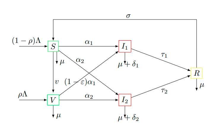
thereby opening the possibility to explore real scenarios that combine the effects of both non-pharmaceutical
public health interventions (e.g., face mask, hand washing, social distancing) and therapeutic measures such
as treatment and mass vaccination strategies [15]. Compartmental models have been crucial to study the
evolution of several disease outbreaks. COVID-19 outbreak has provided a platform for the several research
activities based on compartmental-like epidemic models have been conducted to investigate different key
aspects of the spread, control, and mitigation of the disease [15]. Deterministic compartmental disease
transmission models are characterized by the subdivision of the population into compartments based on
individuals’ health status. The history of mathematical epidemiologic models date as far back as Bernouilli
[16, 17, 18]. Mathematical models of a two-strain disease are numerous in the literature [19]: malaria
[20], influenza [21, 22], SARS-CoV-2 [23], dengue [24], disease with age structure and super-infection [25],
influenza with a single vaccination [26, 29] to cite but a few and the references therein.
    While studies on the dynamics of two viral infections have considered cross-immunity and co-infection
[30], others described effects of two competing strains characterized by cross-immunity [31]. Our proposed
model is a mirror of the two-strain flu model with a single vaccination by [29] and modified by [26] to include
the force of infection in both infected compartments and extending the incidence function to a more general
form. With COVID-19 specificity, we included infections from vaccinated individuals against strain 1, as well
as strain 2, since vaccination against strain 1 may not procure any protection against the second and more
virulent strain 2. Because variant strains have the potential to substantially alter transmission dynamics
and vaccine efficacy, Gonzalez-Parra et al., [23] investigated the impact of more infectious strain of the
transmission dynamics of the COVID-19 pandemic, but they did not consider vaccination. They concluded
that a new variant with higher transmissibility may cause more devastating outcomes in the population.
Our proposed model is seemingly new and to the best of our knowledge, no COVID-19 modelling study has
accounted for strain 1 vaccination with possibility of infection with strain 1 even when vaccinated as well as
infection with strain 2 for which strain 1 vaccination may not provide any protection.
    This paper is organized as follows. We formulate a deterministic compartmental epidemic model of the
transmission dynamics of COVID-19 in a homogeneously mixed population in Section 2. Section 3 is devoted
to well-posedness of the proposed mathematical model, derivation of its equilibria, the basic reproduction
number, and analysis using dynamical systems theory of the COVID-19 transmission dynamics with strain 1
vaccination. Section 4 covers several numerical simulations of the disease dynamics in the presence of strain
1 vaccination in a community where treatment is administered to infected individuals. The and graphical
illustrations are based on various scenarios when the basic reproduction number R0 = max{R1 , R2 } is either
greater or less than unity. The conclusion is provided in Section 5.

2     Model Formulation
It is assumed that the population is homogeneous-mixed and individuals have equal probability of acquiring
the infection. Only human-to-human transmission of COVID-19 is considered. According to individuals dis-
eases status, the human population at time t denoted by Nh (t) is divided into sub-populations of susceptible
individuals S(t), vaccine individuals V1 (t), individuals infected with strain 1 I1 (t), individuals infected with
strain 2 I2 (t) and recovered R(t). The total human population Nh (t) is given by

                                  Nh (t) = S(t) + V (t) + I1 (t) + I2 (t) + R(t).

    Homogeneous mixing of individuals in the population is assumed so that the standard incidence (rate of
                                            1 (t)
infection of strain 1 per unit time) is β1I
                                         N (t)
                                                  . Thus, at any given time t, the probability that an individuals
will carry strain 1 infection is I1N(t) . Infected individuals with strain 1 either die naturally at a constant rare
µ or at a constant disease-induced death rate δ1 . The per capita life expectancy is given by µ1 while µ+δ    1
                                                                                                                1
                                                                                                                  is
the death adjusted average infectious life of a individual infected with strain 1. For simplicity of notations
in what follows, we drop the time t from the model variables.
     While at the onset of the COVID-19 pandemic, the dynamics of the disease was much faster than that
of birth/recruitment and deaths [27] because of the then short period of the pandemic [28], neglecting these
demographic factors was well justified in the plethora of models in the literature. However, since the disease
has been there for a while (since December 2019), at present, it is important to account for the model vital
dynamics when describing the evolution of the COVID-19 pandemic. Therefore, disease-specific death rate
δ1 , δ2 respectively for strain 1 and strain and natural death µ are accounted for. We incorporate both cohort
vaccination (where a fraction ρ of the newly recruited members of the community are vaccinated), and
continuous vaccination program (where a fraction v of susceptible individuals is vaccinated per unit time)
[32].

                                                         2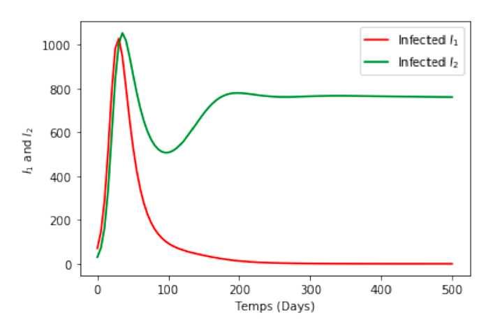
σ
(1 − ρ)Λ α1
S I1
τ1
µ α2
µ + δ1
R
v (1 − ε)α1 µ
τ2
ρΛ α2
V I2
µ µ + δ2
Figure 1: Flowchart of the state progression of individuals in a population exposed to two strains of COVID-19.
At time t, susceptible individuals S(t) can become infected (primary infection) with Strain 1 I1 (t) or Strain
2 I2 (t) or vaccinated against strain 1. Vaccinated individuals V (t) can acquire COVID-19 strain 2. Infected
individuals recover from both strains and move into class R. Recovery is not permanent.
From the conceptual model flow diagram in Figure 1, we derive the following deterministic system of
nonlinear differential equations
Ṡ = (1 − ρ)Λ + σR − (α1 + α2 + µ + v)S,
V̇1 = ρΛ + vS − (α2 + (1 − ε)α1 + µ)V1 ,
I˙1 = α1 S + (1 − ε)α1 V1 − (τ1 + µ + δ1 )I1 , (1)
I˙2 = α2 (S + V ) − (τ2 + µ + δ2 )I2 ,
Ṙ = τ1 I1 + τ2 I2 − (σ + µ)R,
with initial conditions
S(0) ≥ 0, V1 (0) ≥ 0, I1 (0) ≥ 0, I2 (0) ≥ 0, R(0) ≥ 0, (2)
where
I1 I2
α1 = aβ1 , α2 = aβ2 .
N N
The model system (1) involves both exogenous parameters such as the vaccination rate v, and the recov-
ery/treatment rates τ1 and τ2 - the latter represent the inverse of the length in days of the contagious period,
and endogenous parameters such as the disease transmission rate β1 and β2 . The model parameters, their
description, values and sources are provided in the Table 1.
3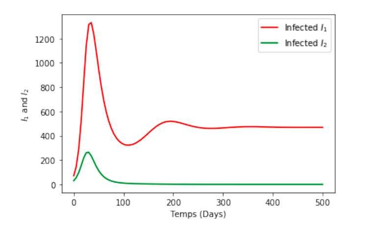
Table 1: Fundamental model parameter
Parameter       Description                                    Value        Range                          Reference

                                                                      1000
Λ               Recruitment or inflow into the population            59×365                                [23, 39]

v               Continuous strain 1 vaccination rate                                  [10−5 , 8 × 10⁻² ]   [40, 41]

a               Effective contact rate                              0.85                                   [46, 47]

β1              Transmission probability of strain 1                                  [0.127, 0.527]       [23, 42]

β2              Transmission probability of strain 2                                  [0.127, 0.527]       [42]

ε               Strain 1 vaccine efficacy                           0.87                                   [43, 44]

                                                                       1
µ               Natural death rate                                   59×365                                [23, 42]

δi              Strain i = {1, 2} disease-induced death rate        6.83 × 10⁻⁵                            [23, 46]

                                                                     1
σ               Rate of loss of immunity                             90                                    [48]

ρ               Cohort vaccination rate                                               (0, 0.99]            [40, 41]

                                                                                        1      1
τ1              Recovery rate of strain 1 infected individuals                        [ 30 ,   4]          [42, 45, 46]

                                                                                        1      1
τ2              Recovery rate of strain 2 infected individuals                        [ 30 ,   4]          [42, 45, 46]

     3     Model analysis
     3.1     Disease-Free equilibrium and basic reproduction number
     For system (1) with non-negative initial values, its solutions are non-negative and ultimately bounded. The
     proof is routine, see for example [28]. Positivity is important for biologically feasible solutions of the model
     while boundedness implies that solutions are finite. Next, we show that the region solutions of model system
     (1) enter in a bounded region Ω.

                                                                        Λ
     Lemma 3.1 The closed set Ω = (S, V1 , I1 , I2 , R) ∈ R5+ : N ≤         is positively invariant and attracting.
                                                                        µ
     Proof. By adding all the equations of the model system (1), we obtain:

                                           Ṅ = Λ − µN − δ1 I1 − δ2 I2 ≤ Λ − µN

                                                                                     Λ           Λ
         Using the comparison theorem as described in [35, 36], we have N (t) ≤        + N (0) −     e−µt
                                                                                     µ           µ
                 Λ                Λ
         If N (0) ≤ then N (t) ≤ . Thus, the region Ω is positively invariant for the model.
                 µ                µ
                 Λ                                                                      Λ
       If N (0) ≥ , then the solution enter in the region Ω in finite time or N (t) →      when t → +∞.
                 µ                                                                       µ
                                                   5
       Thus, the region attracts all solutions in R+ . So the system is positively invariant and attracting.
     Theorem 3.1 The disease free equilibrium of the system (1) is given by E 0 = S 0 , V10 , 0, 0, 0, 0 where


                                           (1 − ρ)Λ           ρΛ + vS 0   (µρ + v)Λ
                                    S0 =            and V10 =           =
                                             µ+v                 µ         µ(µ + v)

                                                                              aβ1 [µ(1 − ρ) + (1 − ε)(µρ + v)]
         The basic reproduction number is R0 = max{R1 , R2 } with R1 =                                         and
                                                                                    (µ + v)(τ1 + µ + δ1 )
                aβ1 [µ(1 − ρ) + (µρ + v)]
         R2 =                             .
                  (µ + v)(τ2 + µ + δ2 )

                                                            4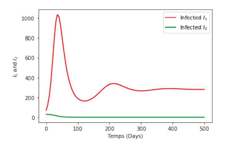
Proof. Using the next generation matrix method in [33] the associated next generation matrix is given by:
I1
aβ1 (S + (1 − ε)V1 )
N
F =
I1
aβ2 (S + V1 )
N
and the rate of transfer of individual to the compartments is given by:
−(τ1 + µ + δ1 )I1
V=
−(τ2 + µ + δ2 )I2
Hence, the new infection terms F and the remaining transfer terms V are respectively given by:
S 0 + (1 − ε)V 0
aβ 1 0
N0
F =
0 0
S + V1
0 aβ2
N0
−(τ1 + µ + δ1 ) 0
V =
0 −(τ2 + µ + δ2 )
S 0 + (1 − ε)V10
aβ 1 0
N 0 (τ1 + µ + δ1 )
F V −1 =
0 0
S + V1
0 aβ2 0
N (τ2 + µ + δ2 )
The dominant eigenvalue or spectral radius of the next generation matrix F V −1 which represents the
basic reproductive number is given by:
S 0 + (1 − ε)V10 S 0 + V10
R0 = max aβ1 0 , aβ2 0 .
N (τ1 + µ + δ1 ) N (τ2 + µ + δ2 )
The basic reproductive number of a disease, denoted R0 is defined as the average number of secondary
infections that a single infectious individual will give rise to over the duration of his infection, in an otherwise
entirely susceptible population.
Let
S 0 + (1 − ε)V10 aβ1 [µ(1 − ρ) + (1 − ε)(µρ + v)]
R1 = aβ1 0 =
N (τ1 + µ + δ1 ) (µ + v)(τ1 + µ + δ1 )
and
S 0 + V10 aβ1 [µ(1 − ρ) + (µρ + v)]
R2 = aβ2 =
N 0 (τ2 + µ + δ2 ) (µ + v)(τ2 + µ + δ2 )
Then
R0 = max{R1 , R2 }
Theorem 3.2 The disease-free equilibrium E 0 is unstable if R0 > 1 while it is locally asymptotically stable
if R0 < 1.
Proof.
The Jacobian matrix associated with the model system (1) at the disease-free equilibrium is given by:
S0 S0
−(µ + v) 0 −aβ1 −aβ2 σ
N0 N0
V10 V10
v −µ −a(1 − ε)β1 −aβ2 0
N0 N0
(S 0 + (1 − ε)V10 )
JE 0 =
0 0 aβ1 − (τ1 + µ + δ1 ) 0 0
N0
S 0 + V10
0 0 0 aβ2 − (τ2 + µ + δ2 ) 0
N0
0 0 τ1 τ2 −(σ + µ)
5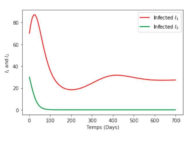
S0 S0
−(µ + v) 0 −aβ1
N0
−aβ2
N0
σ
V10 V10
v −µ −a(1 − ε)β1 −aβ2 0
N0 N0
JE 0 =
0 0 (τ1 + µ + δ1 )(R1 − 1) 0 0
0 0 0 (τ2 + µ + δ2 )(R2 − 1) 0
0 0 τ1 τ2 −(σ + µ)
Thus the eigenvalues of JE 0 are λ1 = −(µ + v), λ2 = −µ, λ3 = −(σ + µ), λ4 = (τ1 + µ + δ1 )(R1 −
1) and λ5 = (τ2 + µ + δ2 )(R2 − 1).
If R0 < 1, then λ4 , λ5 < 0 and we obtain that the disease-free equilibrium E 0 of Model (1) is locally
asymptotically stable. If R0 > 1, then the disease-free equilibrium loses its stability.
Theorem 3.3 The disease-free equilibrium E 0 is globally asymptotically stable if, R0 > 1.
Proof. Consider the Lyapunov function
V (S, V1 , I1 , I2 ) = I1 + I2 ,
Since I1 , I2 > 0, then V (S, V1 , I1 , I2 ) > 0 and V (S, V1 , I1 , I2 ) attains zero at I1 = I2 = 0.
Now, we need to show V̇ ≤ 0.
V̇ = I˙1 + I˙2
aβ1 I1 aβ1 I1 aβ2 I2
= S + (1 − ε) V1 − (τ1 + µ + δ1 )I1 + (S + V1 ) − (τ2 + µ + δ2 )I2 (3)
N N N
aβ1 (S + (1 − ε)V1 ) aβ2 (S + V1 )
= (τ1 + µ + δ1 )I1 − 1 + (τ2 + µ + δ2 )I2 −1
N (τ1 + µ + δ1 ) N (τ2 + µ + δ2 )
Because S 0 ≤ 0 and V10 ≤ 0 then
V̇ ≤ (τ1 + µ + δ1 )I1 (R1 − 1) + (τ2 + µ + δ2 )I1 (R2 − 1) ≤ 0
dV
Furthermore, = 0 if and only if I1 = I2 = 0, so by using the LaSalle’s invariant principle, this implies
dt
that E0 is globally asymptotically stable in Ω.
Remark Using the standard comparison theorem as described in [35, 36] and rigorously applied in
[37, 38, 39], this result can also be proved (see appendix A).
3.2 Endemic equilibrium
Theorem 3.4 The model (1) admits
1. a unique single-strain 1 infection equilibrium E1 = (S ∗ , V1∗ , I1∗ , 0, R∗ ) if and only if R1 > 1.
2. a unique single-strain 2 infection equilibrium E2 = (S ∗ , V1∗ , 0, I2∗ , R∗ ) if and only if R2 > 1.
3. a 2-strain infection equilibrium E3 = (S ∗ , V1∗ , I1∗ , I2∗ , R∗ ) when R0 = max{R1 , R2 } > 1.
Proof. (1) Equilibrium E1 is the solution of the system
(1 − ρ)Λ + σR∗ − (α1 + µ + v)S ∗ = 0,
∗ ∗
ρΛ + vS − ((1 − ε)α1 + µ)V1 = 0,
(4)
α1 S ∗ + (1 − ε)α1 V1∗ − (τ1 + µ + δ1 )I1∗ = 0,
τ1 I1∗ − (σ + µ)R∗ = 0,
From the first three equations in 4 above, the model system (1) admits a unique single-strain 1 infection
equilibrium E1 = (S ∗ , V1∗ , I1∗ , 0, R∗ ) if and only if R1 > 1 given by
(1 − ρ)Λ + σR∗
S∗ = ,
α1∗ + µ + v
ρΛ + vS ∗
V∗ = ,
(1 − ε)α1∗ + µ
6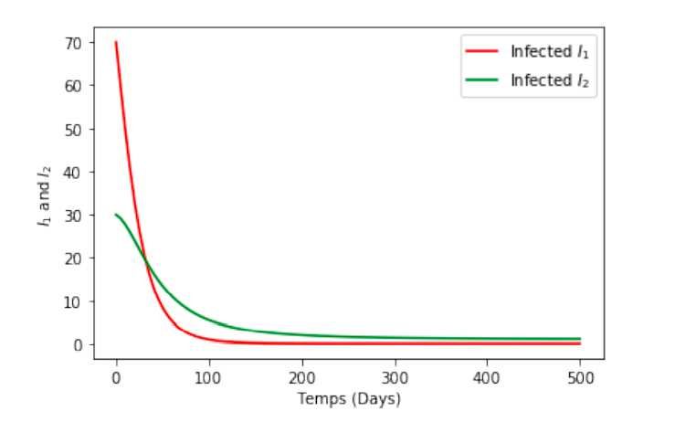
α1 S ∗ + (1 − ε)α1∗ V ∗
I1∗ = .
τ1 + µ + δ 1
Using the last equation of the system 4 and the definition of α1∗ , we obtain after some algebraic calculation
that α1∗ is the solution of the equation
α1∗ (c2 α1∗2 + c1 α1∗ + c0 ) = 0, (5)
where
c2 = (1 − ε1 )(µ + σ + τ1 ) > 0,
c1 = (µ + σ + τ1 )(µ + (1 − ε)v) + (µ + σ) [δ1 ρ + (1 − ε)(µ + τ1 + δ1 (1 − ρ) − aβ1 )] , (6)
c0 = (µ + σ)(µ + v)(µ + τ1 + δ1 )(1 − R1 ).
When R1 > 1, c0 < 0 and the discriminant of the quadratic equation 5 is given by ∆ = c21 − 4c0 c2 > 0,
c0
and thus equation 5 admits two reals solutions. In addition, the product of those two solutions is p = < 0,
c2
implying that the two solutions have different signs. Hence, we can conclude that when R1 > 1, the system
admit a unique single-strain 1 infection equilibrium.
(2) The proof follows the same approach and steps as in the above case (1).
(3) To find E3 , we consider the system
(1 − ρ)Λ + σR∗ − (α1∗ + α2∗ + µ + v)S ∗ = 0,
ρΛ + vS ∗ − (α2∗ + (1 − ε)α1∗ + µ)V1∗ = 0,
α1∗ S ∗ + (1 − ε)α1∗ V1∗ − (τ1 + µ + δ1 )I1∗ = 0, (7)
α2∗ (S ∗ + V1∗ ) − (τ2 + µ + δ2 )I2∗ = 0,
τ1 I1∗ + τ2 I2∗ − (σ + µ)R∗ = 0,
aβ1 I1∗ aβ2 I2∗ Λ + δ1 I1∗ + δ2 I2∗
where α1∗ = , α2∗ = with N ∗ = . After some algebraic manipulations we
N ∗ N ∗ µ
∗ ∗ ∗
τ 1 I1 + τ 2 I2 (1 − ρ)Λ + σR ρΛ + vS ∗
obtain R∗ = , S∗ = ∗ , and V1∗ = ∗ .
σ+µ α1 + α2 + µ + v
∗
α2 + (1 − ε)α1∗ + µ
∗ ∗ ∗
Replacing S ; V1 and R with their values in the third and fourth equation yields the following system
∗ ∗
f (I1 , I2 ) = 0,
(8)
g(I1∗ , I2∗ ) = 0,
where f and g are monotone functions defined by
I1 aβ1 (1 − ε) I1 Λaβ1 µρ + I1 Λaβ1 ρσ + I1 N στ1 v + I2 Λaβ2 µρ + I2 Λaβ2 ρσ + I2 N στ2 v + ΛN µ2 ρ + ΛN µρσ + ΛN µv + ΛN σv
f (I1∗ , I2∗ ) = −
(µ + σ) (I1 aβ1 + I2 aβ2 + N µ + N v) (I1 aβ1 ǫ − I1 aβ1 − I2 aβ2 − N µ)
I1 aβ1 (I1 στ1 + I2 στ2 − Λµρ + Λµ − Λρσ + Λσ)
+ − I1 (δ1 + µ + τ1 ) ,
(µ + σ) (I1 aβ1 + I2 aβ2 + N µ + N v)
I2 aβ2 I1 Λaβ1 µρ + I1 Λaβ1 ρσ + I1 N στ1 v + I2 Λaβ2 µρ + I2 Λaβ2 ρσ + I2 N στ2 v + ΛN µ2 ρ + ΛN µρσ + ΛN µv + ΛN σv
g(I1∗ , I2∗ ) = −
(µ + σ) (I1 aβ1 + I2 aβ2 + N µ + N v) (I1 aβ1 ǫ − I1 aβ1 − I2 aβ2 − N µ)
I2 aβ2 (I1 στ1 + I2 στ2 − Λµρ + Λµ − Λρσ + Λσ)
+ − I2 (δ2 + µ + τ2 ) .
(µ + σ) (I1 aβ1 + I2 aβ2 + N µ + N v)
If the system (8) admits a solution, then, the model system (1) will have an endemic equilibrium.
Obtaining the explicitly expression for the exact solution of the non-linear autonomous system (8) is a
daunting task. Also, it not obvious if the system (8) admits multiple solutions, it therefore is important to
explore the uniqueness and global stability of the 2-strain endemic equilibrium. To this end, we investigate
if the model system (8) undergoes the phenomenon of backward bifurcation where a stable disease-free
equilibrium with a stable endemic equilibrium co-existence when R0 < 1.
3.3 Bifurcation analysis
In determining the possibility of backward bifurcation occurring, we use the centre manifold theory approach
[34]. For simplification of the notations and ease of algebraic manipulations, the following change of variables
is made. Let S(t) = x1 , V (t) = x2 , I1 (t) = x3 , I2 (t) = x4 and R(t) = x5 , by using the vector notation
7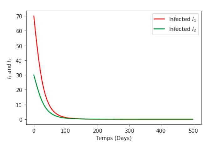
x = (x1 , x2 , x3 , x4 , x5 )T (where T denote the transpose), our model system (8) can be written in the form
dx
= f (x) with f (x) = (f1 , f2 , f3 , f4 , f5 )T as follows:
dt
ẋ1 = f1 (x) = (1 − ρ)Λ + σx5 − (α1 + α2 + µ + v)x1 ,
ẋ2 = f2 (x) = ρΛ + vx1 − (α2 + (1 − ε)α1 + µ)x2 ,
ẋ3 = f3 (x) = α1 x1 + (1 − ε)α1 x2 − (τ1 + µ + δ1 )x3 , (9)
ẋ4 = f4 (x) = α2 (x1 + x2 ) − (τ2 + µ + δ2 )x4 ,
ẋ5 = f5 (x) = τ1 x3 + τ2 x4 − (σ + µ)x5 ,
x3 x4
where α1 = aβ1 and α2 = aβ1 .
x1 + x2 + x3 + x4 + x5 x1 + x2 + x3 + x 4 + x 5
The Jacobian of the system (9) at the DFE is given by
µ(1 − ρ) µ(1 − ρ)
−(µ + v) 0 −aβ1 −aβ2 σ
µ+v µ+v
µρ + v µρ + v
v −µ −a(1 − ε)β1 −aβ2 0
µ+v µ+v
JE 0 = . (10)
0 0 (τ1 + µ + δ1 )(R1 − 1) 0 0
0 0 0 (τ2 + µ + δ2 )(R2 − 1) 0
0 0 τ1 τ2 −(σ + µ)
aβ1 [µ(1 − ρ) + (1 − ε)(µρ + v)]
First, consider the case R = R1 = .
(µ + v)(τ1 + µ + δ1 )
Consider the case when R1 = 1, which is the bifurcation point. Suppose, further that β1 = β1∗ is chosen
(µ + v)(τ1 + µ + δ1 )
as a bifurcation parameter. Solving for β1 from R1 = 1 gives β1∗ =
a [µ(1 − ρ) + (1 − ε)(µρ + v)]
µ(1 − ρ) µ(1 − ρ)
−(µ + v) 0 −aβ1∗ −aβ2 σ
µ+v µ+v
∗ µρ + v µρ + v
v −µ −a(1 − ε)β 1 −aβ 2 0
µ+v µ+v
J β1 = . (11)
∗
0 0 0 0 0
0 0 0 (τ 2 + µ + δ 2 )(R 2 − 1) 0
0 0 τ1 τ2 −(σ + µ)
When R1 = 1, the Jacobian of (9) at β1 = β1∗ c (denoted by Jβ1∗ ) has a right eigenvector given by w =
µp3 (µ + σ) + v[(µ + σ)(p1 + p3 ) + στ1 ] (µ + σ)(µ + v)
[w1 , w2 , w3 , w4 , w5 ]T , where, w1 = 1, w2 = , w3 = ,
µ[στ1 + (µ + σ)p1 ] στ1 + (µ + σ)p1
τ1 (µ + v) µ(1 − ρ) µ(1 − ρ) µρ + v
w4 = 0 and w5 = , where p1 = −aβ1∗ , p2 = −aβ2 , p3 = −a(1 − ε)β1∗
στ1 + (µ + σ)p1 µ+v µ+v µ+v
µρ + v
and p4 = −aβ2 .
µ+v
Further, the Jacobian Jβ1∗ has a left eigenvector v = [v1 , v2 , v3 , v4 , v5 ]T , where v1 = v2 = v4 = v5 = 0 =,
v3 = 1.
5
X ∂ 2 fk
a = vk w i w j (E0 , β1∗ ),
∂xi ∂xj
k,i,j=1
w3 aβ1∗ (1 + x∗1 + (1 − ε)x∗2 )
= − ,
(x∗1 + x∗2 )2
After some algebraic computations, we obtain
β1∗ (µ + σ)(µ + v)(1 + x∗1 + (1 − ε)x∗2 )
a=− ∗ 2
στ1 (x∗1 + x2 ) [µ(1 − ρ)(1 − (τ + µ + δ1 )) + (1 − ε)(µρ + v)]
It is evident that a < 0, since 1 − ε > 0, 1 − ρ > 0 and 1 − (τ1 + µ + δ1 ) > 0.
8The second bifurcation coefficient b is given by
5
X ∂ 2 fk
b = vk w j (E0 , β1∗ ),
∂xj ∂βm
k,j=1
a(x∗1 + (1 − ε)x∗2 )
= >0
x∗1 + x∗2
Because a is negative and b is positive, and by Theorem 4.1 in [34], this precludes the model system (8) from
exhibiting the phenomenon of backward bifurcation at R0 = 1. Consequently, the following results holds.
Lemma 3.2 The unique endemic equilibrium E3 of the model system 1 is globally asymptotically stable if
R0 > 1.
4 Numerical simulations
To illustrate the basic mechanisms underlying the model dynamics, several graphical representations depict-
ing the dynamical behavior of the model system 1 when the fundamental threshold parameter R0 is either
greater or less than unity are presented to support the analytical results. The model parameter values used in
our simulations are shown in Table 1. The unit of Λ is person per day while all other parameters’ unit is per
day. We consider the following initial conditions: (S(0) = 5000, V1 (0) = 100, I1 (0) = 70, I2 (0) = 30, R(0) =
5. Because R0 = max{R1 , R2 }, four scenarios will be considered. Note that values of our proposed COVID-
19 model’s basic reproduction number R0 = max{R1 , R2 } (with R1 and R2 denoting respectively the strain
1 and strain 2 basic reproduction) are in agreement with previous COVID-19 modeling studies [49, 50, 51].
4.1 Simulation when R0 > 1 with R1 > 1 and R2 > 1
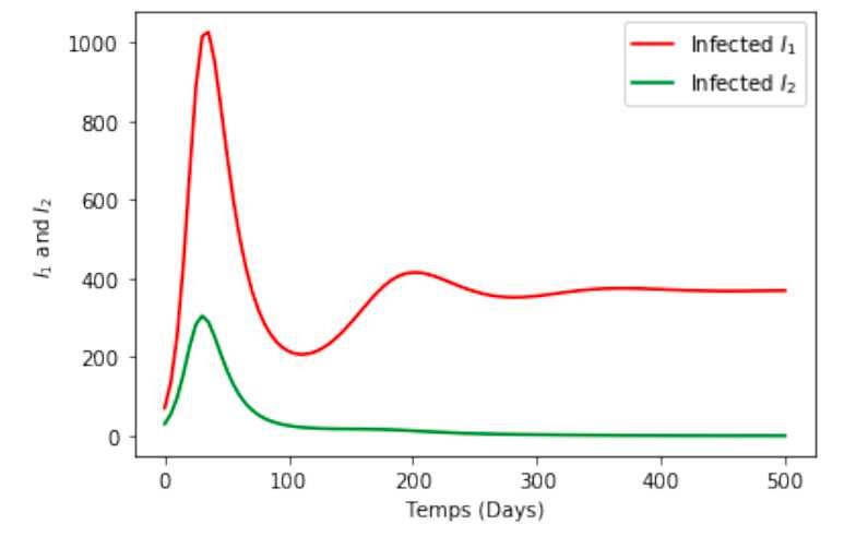
Time series solution of two infected classes I1 (t) and I2 (t) are plotted in Figures 2 and 3 when R0 > 1 with
R1 < R2 . In this case, the solutions of the model system 1 approach the equilibria E3 . These graphs show
the occurrence of a second wave as predicted in [10], and possibly a third wave. However, we note that under
very pessimistic conditions with availability of only strain 1 vaccine, strain 2 could become the dominant
strain in the population if infections with strain 2 are more than double that of strain 1, see Figure 3.
Figure 2: Simulations showing individuals Figure 3: Simulations showing individuals
I1 and I2 for R1 = 2.48 and R2 = 8.58 I1 and I2 for R1 = 1.29 and R2 = 4.78
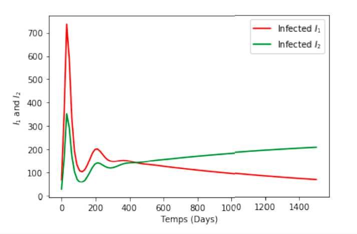
4.2 Simulation when R0 > 1 with R1 < 1 and R2 > 1
Figures 4 and 5 depict the case when R0 > 1 with R1 < 1 and R2 > 1. As depicted in Figure 5, at the
long run, strain 2 could establish itself as the dominant strain in the population. Note that in this case, the
solution profiles approach the equilibrum E2
9Figure 4: Simulations showing individuals Figure 5: Simulations showing individuals
I1 and I2 for R1 = 0.77 and R2 = 1.0037 I1 and I2 for R1 = 0.92 and R2 = 2.27
4.3 Simulation when R0 > 1 with (a) R1 > 1 and R2 < 1 and (b) R1 = R2
Figures 6 and 7 display respectively the cases when (a) R0 > 1 with R1 < 1 and R2 > 1 (left panel) and
(b) R1 = R2 (right panel). Again, the dynamical behavior of the graph of strain 1 depict multiple waves.
In both cases (a) and (b), strain 2 will not establish itself in the population as the solutions approach
the equilibrium E1 . It is surprising to notice that when both strain 1 and strain 2 reproduction numbers
are equal and greater than unity, strain 2 could eventually die out. Several reasons could explain this.
First, strain 2 emerged in the population when efforts to mitigate the strain 1 such as non-pharmaceutical
interventions (including physical distancing, hand hygiene, and mask-wearing) as well as treatment were
already well underway. Secondly, continuous vaccination against strain 1 could likely confer some protection
to individuals against strain 2. In this case,
Figure 6: Simulations showing individuals
I1 and I2 for R1 = 1.92 and R2 = 0.94
Figure 7: Simulations showing individuals I1 and I2 for R1 = R2 = 2.27
104.4 Simulation when R0 < 1
When R0 < 1, that is both R1 and R2 are less than unity with R1 < R2 , the evolutionary dynamics of the
solutions approach the disease-free equilibrium E0 , see Figure 8. On the other hand, when R0 < 1 with
R1 > R2 , it is striking to note that because R1 is very closed to 1, Figure 9, the strain infection I1 will
not be quickly eradicated, and efforts to further reduce the average number of infections from a susceptible
individual in a totally susceptible population is warranted.
Figure 8: Simulations showing individuals Figure 9: Simulations showing individuals
I1 and I2 for R1 = 0.77 and R2 = 0.91 I1 and I2 for R1 = 0.96 and R2 = 0.91
5 Conclusion
COVID-19 emerged in December 2019, has rapidly evolved as a pandemic with wide-ranging socio-economic
consequences. The disease causes severe acute respiratory syndrome and results in substantial morbidity
and mortality. While an effective vaccine is essential to containing the spread COVID-19, the emergence
of a second strain could complicate mitigation efforts. We developed a simple compartment model of the
transmission dynamics of a 2-strain of COVID-19 model to examine the impact strain 2 in a population where
vaccination against strain 1 is available. The proposed 2-strain COVID-19 model with strain 1 vaccination
is derived as a deterministic system of nonlinear differential equations. The model is then theoretically
analyzed, its basic reproduction number R0 is derived as well as sufficient conditions for the stability of its
equilibria. We calculate the basic reproductive numbersR1 and R2 for both strains independently. Using
the center manifold theory, it is shown that the model does not exhibit bi-stability also known as backward
bifurcation, and global stability of the model equilibria when R0 is either less or greater than unity is establish
using a suitably constructed Lyapunov function and other approaches such as the comparison method.
To gain insight into whether strain will establish itself in the population as the dominant strain, several
simulations to support the model theoretical results are provided. Results indicate that - both strains will
persist when both R1 > 1 and R2 > 1 - Stain 2 could likely establish itself as the dominant strain if R1 < 1
and R2 > 1, or when R2 is at least two times R1 . However, with the current knowledge of the epidemiology
of the COVID-19 pandemic and the availability of treatment effective vaccine against strain 1, strain 2 is
would eventually be eradicated in the population if the threshold parameter R2 is controlled to remain below
unity. We note that if we ignore the model vital dynamics (recruitment and natural death) to mimic the
ongoing epidemic, there is no noticeable impact on the dynamical behavior of the figures. There are however
some contrasting findings with respect to the value of the basic reproduction number.
(i) Under a very pessimistic condition, strain 2 could become the dominant strain in the population if
infections with strain 2 are more than double that of strain 1, see Figure 3.
(ii) When both strain 1 and strain 2 reproduction numbers are equal and greater than unity, strain 2 could
eventually die out while strain 1 persists.
From observation (ii), while R0 provides a good measure for disease dying out or persisting in a pop-
ulation, this threshold quantity when less than but close to unity might mislead the assessment of the
transmission dynamics of the disease. Thus, ensuring that the value of R0 is below unity may depend on
how far from unity this value is in order to ascertain how quickly the disease eventually dies out. That is,
even though the model does not exhibit the possibility of bi-stable behavior of its equilibria, strain 1 could
persist for some time when R1 < 1, but close to 1. From this finding and in the face of waning adherence
to physical distancing, the use of non-pharmaceutical interventions the word has relied upon (such as lock-
downs, travel restrictions, contact tracing, mask wearing, and social/physical distancing), and the emergence
of other COVID-19 variants, it is cautionary to ensure decision on relaxing/lifting these non-pharmaceutical
prevention measures are not solely based on the value of the basic reproduction number being less than
unity, but considerations should be made on how close to 1 this value actually is as well as other socio and
11eco-epidemiological factors pertaining to the dynamics of COVID-19, and also account for regional hetero-
geneity in transmission and travel. Nevertheless, there is a glimpse of hope that if individuals concurrently
continue to adhere to non-pharmaceutical interventions (including physical distancing, hand hygiene, and
mask-wearing), and other pharmaceutical efforts to mitigate the strain 1 such as treatment and vaccination
continue, strain 2 could be eradicated.
The proposed model has some limitations. While co-infection of the COVID-19 has not been a major
issue, from a theoretical standpoint, the model could be extended to include the latent class and individuals
dually infected with both strain 1 and strain 2. In this case, one could compute the invasion reproductive
number for strain 1 when strain 2 is at endemic equilibrium and vice-versa [52]. Due to the severity of the
disease, explicitly incorporating the quarantine and hospitalized class is viable. While these suggestions will
increase the complexity of the model analysis, by construction, there are often uncertainty around some
parameter values, and a detailed uncertainty and sensitivity analyses to determine the parameters that have
the highest effect on the model variables should also be considered.
Conflicts of interest/Competing interests The authors declare that they have no conflict of interest.
Availability of data and material All data (model parameter values) used in this work are in the
text and Table 1.
Code availability The routine Python code used in this work can be made available upon
request to the authors.
Funding None
References
[1] VD Menachery, BL Yount Jr, K Debbink, S Agnihothram, LE Gralinski, JA Plante, RL
Graham, T Scobey, Xing-Yi Ge, EF Donaldson, et al. A SARS-like cluster of circulating
bat coronaviruses shows potential for human emergence. Nature Medicine, 21(12), 1508
(2015).
[2] World Health Organization et al. Coronavirus disease 2019 (covid-19): situation report,
67 (2020).
[3] Qun Li, Xuhua Guan, Peng Wu, Xiaoye Wang, Lei Zhou, Yeqing Tong, Ruiqi Ren,
Kathy SM Leung, Eric HY Lau, Jessica Y Wong, et al. Early transmission dynamics
in Wuhan, China, of novel coronavirus-infected pneumonia. New England Journal of
Medicine (2020).
[4] M Cascella, M Rajnik, A Cuomo, SC Dulebohn, R Di Napoli. Features, evaluation and
treatment coronavirus (Covid-19). In StatPearls [Internet]. StatPearls Publishing (2020).
[5] Vital Surveillances. The epidemiological characteristics of an outbreak of 2019 novel coro-
navirus diseases (Covid-19)-China, 2020. China CDC Weekly, 2(8), 113-122 (2020).
[6] Z Wu, JM McGoogan. Characteristics of and important lessons from the coronavirus
disease 2019 (covid-19) outbreak in china: summary of a report of 72 314 cases from the
Chinese center for disease control and prevention. JAMA (2020).
[7] Coronavirus disease (COVID-19) outbreak situation, https :
//www.who.int/emergencies/diseases/novel − coronavirus − 2019, April (2020).
[8] Gumel AB, Iboi EA, Ngonghala C.N. Elbasha E.H., A primer on using mathematics
to understand COVID-19 dynamics: Modeling, analysis and simulations, Inf. Dis. Mod.
(2020).
[9] S. Usaini, A. S. Hassan, S. M. Garba JM-S. Lubuma. Modeling the transmission dy-
namics of the Middle East Respiratory Syndrome Coronavirus (MERS-CoV) with latent
immigrants. J. Interdisciplinary Math. 22(6), 903-930 (2019).
[10] Pedro SA, Ndjomatchoua FT, Jentsch P, Tchuenche JM, Anand M, Bauch CT. Conditions
for a second wave of COVID-19 due to interactions between disease dynamics and social
processes. Front. Phys. 8, 574514 (2020).
[11] PC Jentsch, M Anand, CT Bauch. Prioritising COVID-19 vaccination in changing so-
cial and epidemiological landscapes: a mathematical modelling study. Lancet Infectious
Diseases (2021). https : //doi.org/10.1016/S1473 − 3099(21)00057 − 8
12[12] JP Olumuyiwa, S. Qureshi, A Yusuf, M Al-Shomrani, AA Idowu. A new mathematical
model of COVID-19 using real data from Pakistan. Results in Physics, 24, 104098 (2021).
[13] JH Buckner, G Chowell, MR Springborn. Dynamic prioritization of COVID-19 vac-
cines when social distancing is limited for essential workers, Proceedings of the National
Academy of Sciences 118(16), e2025786118 (2021).
[14] Saad-Roy CM, Wagner CE, Baker RE, et al. Immune life history, vaccination, and the
dynamics of SARS-CoV-2 over the next 5 years. Science 370, 811-818 92020).
[15] A Olivares, E Staffetti. Uncertainty quantification of a mathematical model of COVID-19
transmission dynamics with mass vaccination strategy. Chaos, Solitons & Fractals 146,
110895 (2021).
[16] Bernoulli D. Essai d’une nouvelle analyse de la mortalitecausee par la petite verole et des
avantages de l’inoculation pour la prevenir. Me.m Math. Phys. Acad. R. Sci. Paris, 1-45
(1766).
[17] Kermack WO, McKendrick AG. A contribution to the mathematical theory of epidemics.
Proc. R. Soc. Lond. Ser. A, 115(772), 700-721 (1927).
[18] Dietz K, Heesterbeek JAP. Daniel Bernoulli’s epidemiological model revisited. Math
Biosci. 180(1-2), 1-21 (2002).
[19] M Nuno, C Castillo-Chavez, Z Feng, M Martcheva. Mathematical models of influenza:
The role of cross-immunity, quarantine and age-structure. in: Brauer F., van den Driess-
che P., Wu J. (eds) Mathematical Epidemiology. Lecture Notes in Mathematics, vol 1945.
Springer, Berlin, Heidelberg (2008).
[20] Bala S, Gimba B. Global sensitivity analysis to study the impacts of bed-nets, drug
treatment, and their efficacies on a two-strain malaria model, Math. Comput. Appl.
24(1), 32 (2019).
[21] Chung KW, Lui R. Dynamics of two-strain influenza model with cross-immunity and no
quarantine class. J Math Biol. 73(6-7), 1467-1489 (2016).
[22] F Chamchod, NF Britton. On the dynamics of a two-strain influenza model with isolation.
Math. Model. Nat. Phenom. 7 (3) 49-61 (2012).
[23] Gonzalez-Parra G, Martinez-Rodriguez D, Villanueva-Mico RJ. Impact of a new SARS-
CoV-2 variant on the population: A mathematical modeling approach, Math. Comput.
Appl. 26(2), 25 (2021).
[24] P Rashkov, BW Kooi Complexity of host-vector dynamics in a two-strain dengue model,
J. Biol. Dyn. 15(1), 35-72 (2021).
[25] Li XZ, Liu JX, Martcheva M. An age-structured two-strain epidemic model with super-
infection, Math. Biosci. Eng. 7(1), 123-147 (2010).
[26] Nic-May AJ, Avila-Vales EJ. Global dynamics of a two-strain flu model with a single
vaccination and general incidence rate, Math. Biosci. Eng. 17(6), 7862-7891 (2020).
[27] Kroger M, Schlickeiser R. Analytical solution of the SIR-model for the temporal evolution
of epidemics. Part A: time-independent reproduction factor, J. Phys. A: Math. Theor. 53
505601 (2020).
[28] Song H, Jia Z, Jin Z. et al. Estimation of COVID-19 outbreak size in Harbin, China,
Nonlinear Dyn. (2021).
[29] SM Ashrafur Rahman, X Zou Flu epidemics: a two-strain flu model with a single vacci-
nation, J. Biol. Dyn. 5(5), 376-390 (2011).
[30] L. Allen, M. Langlais and C. J. Phillips, The dynamics of two viral infections in a single
host population with applications to hantavirus, Math. Biosci. 186, 191-217 (2003).
[31] M. Nuno, G. Chowell, X. Wang and C. Castillo-Chavez, On the role of cross-immunity
and vaccines on the survival of less fit flu strains, Theor. Pop. Biol. 71,20-29 (2007).
[32] Rwezaura H, Mtisi E, Tchuenche JM. A Mathematical analysis of influenza with treat-
ment and vaccination. In: Infectious Disease Modelling Research Progress, Series - Public
Health in the 21st Century, J.M. Tchuenche and C. Chiyaka (eds) Nova Science Publish-
ers, NY, Inc, pp. 31-84 (2010).
[33] van den Driessche P, Watmough J. Reproduction numbers and sub-threshold endemic
equilibria for compartmental models of disease transmission, Math. Biosci. 180(1), 29-48
(2002).
[34] Castillo-Chavez C , Song B . Dynamical models of tuberculosis and their applications,
Math. Biosci. Eng. 1(2), 361-404 (2004).
13[35] V. Lakshmikantham, S. Leela, A. A. Martynyuk. Stability Analysis of Nonlinear Systems,
Marcel Dekker, Inc., New York and Basel (1989).
[36] H.L. Smith and P. Waltman. The Theory of the Chemostat, Cambridge University Press
(1995).
[37] Mtisi E, Rwezaura H, Tchuenche JM. A mathematical analysis of malaria and tuberculosis
co-dynamics, Discrete Cont. Dyn. Syst. B, 12(4), 827-864 (2009).
[38] Sharomi O, Gumel AB. Curtailing smoking dynamics: A mathematical modeling ap-
proach, Appl. Math. Comput. 195, 475-499 (2008).
[39] Agusto FB, Gumel AB. Theoretical assessment of avian influenza vaccine, Discrete Cont.
Dyn. Syst. B 13(1), 1-25 (2009).
[40] Elbasha EH, Gumel AB. Theoretical assessment of public health impact of imperfect
prophylactic HIV-1 vaccines with therapeutic benefits, Bull. Math. Biol. 68(3), 577-614
(2006).
[41] Rabiu M, Willie R, Parumasur N. Mathematical analysis of a disease-resistant model
with imperfect vaccine, quarantine and treatment, Ricerche di Matematica 69, 603-627
(2020).
[42] Mwalili S, Kimathi M, Ojiambo V, Gathungu D, Mbogo R. SEIR model for COVID-19
dynamics incorporating the environment and social distancing, BMC Res. Notes. 13(1),
352 (2020).
[43] Thompson MG, Burgess JL, Naleway AL, et al. Interim estimates of vaccine effectiveness
of BNT162b2 and mRNA-1273 COVID-19 vaccines in preventing SARS-CoV-2 infection
among health care personnel, first responders, and other essential and frontline workers
- Eight U.S. locations, December 2020-March 2021. MMWR Morb. Mortal. Wkly. Rep.
70, 495-500 (2021).
[44] Pilishvili T, Fleming-Dutra KE, Farrar JL, et al. Interim estimates of vaccine effectiveness
of Pfizer-BioNTech and Moderna COVID-19 vaccines among health care personnel - 33
U.S. sites, January-March 2021. MMWR Morb. Mortal. Wkly. Rep. 70, 753-758 (2021).
[45] Ngonghala CN, Iboi E, Eikenberry S, Scotch M, MacIntyre CR, Bonds MH, Gumel AB,
Mathematical assessment of the impact of non-pharmaceutical interventions on curtailing
the 2019 novel coronavirus, Math. Biosci. 325 (2020).
[46] Garba SM, Lubuma JM, Tsanou B. Modeling the transmission dynamics of the COVID-
19 Pandemic in South Africa, Math. Biosci. 328, 108441 (2020).
[47] Ivorra B, Ferrandez MR, Vela-Perez M, Ramos AM. Mathematical modeling of the spread
of the coronavirus disease 2019 (COVID-19) taking into account the undetected infections.
The case of China. Commun. Nonlinear. Sci. Numer. Simul. 88, 105303 (2020).
[48] Getachew TT, Haileyesus TA. Mathematical modeling and optimal control analysis of
COVID-19 in Ethiopia, J. Interdisciplinary Math. DOI : 10.1080/09720502.2021.1874086
(2021).
[49] Dharmaratne S, Sudaraka S, Abeyagunawardena I, Manchanayake K, Kothalawala M,
Gunathunga W. Estimation of the basic reproduction number (R0) for the novel coron-
avirus disease in Sri Lanka, Virol. J. 17(1), 144 (2020).
[50] Linka K, Peirlinck M, Kuhl E. The reproduction number of COVID-19 and its correlation
with public health interventions, Comput. Mech. 1-16 (2020).
[51] Subramanian R, He Q, Pascual M. Quantifying asymptomatic infection and transmission
of COVID-19 in New York City using observed cases, serology, and testing capacity, Proc.
Natl. Acad. Sci. U S A. 118(9), e2019716118 (2021).
[52] Crawford B, Kribs-Zaleta CM. The impact of vaccination and coinfection on HPV and
cervical cancer, Discrete Cont. Dyn. Syst. B, 12(2), 279-304 (2009).
Appendix A: GAS of DFE using comparaison theorem
The following results provides an alternate proof to theorem 3.3.
Theorem 5.1 The disease-free equilibrium E 0 is globally asymptotically stable if, R0 > 1.
Proof. The proof is based applying a standard comparison theorem as described in [35, 36]
and applied in [37, 38, 39]. The equations for the infected components in (1) can be written
in terms of
′
I1 (t) I1 (t) I1 (t) I1 (t)
= (F − V ) − M 1 Q1 − M2 Q2 , (12)
I2′ (t) I2 (t) I2 (t) I2 (t)
14S + (1 − ε)V1 N0
where F and V are matrices defined in section 3.1, M1 = 1 − × 0 ,
N S + (1 − ε)V10
S + V1
M2 = 1 − and Q1 and Q2 are non-negative matrices given respectively by
N
aβ1 (S 0 + (1 − ε)V10 )
0 0 0
N 0
Q1 = , Q2 = .
0 0 0 aβ 2
S(t) + (1 − ε)V1 (t) N0
Thus, since S(t)+V1 (t) ≤ N (t) and assuming that for all t ≥ 0, × 0 ≤
N (t) S + (1 − ε)V10
1 in Ω, it follows from 12 that
I1′ (t) I1 (t)
≤ (F − V ) . (13)
I2′ (t) I2 (t)
Using the fact that the eigenvalues of the matrix F − V all have negative real parts, it follows
that the linearized differential inequality system (13) is stable whenever R0 < 1. Consequently,
(I1 (t), I2 (t)) → (0, 0) as t → ∞. Thus, by comparison theorem [35, 36], (I1 (t), I2 (t)) → (0, 0) as
t → ∞. Substituting I1 = I2 = 0 in the first and second equations of the model 1 gives S(t) → S 0
and V1 (t) → V10 as t → ∞. Thus, (S(t), V1 (t), I1 (t), I1 (t), R(t)) → (S 0 , V10 , 0, 0, 0) as t → ∞ for R0 < 1.
Hence, the DFE E 0 is GAS in Ω if R0 < 1.
15Figures Figure 1 Please see the Manuscript PDF le for the complete gure caption
Figure 2

Please see the Manuscript PDF le for the complete gure caption
Figure 3

Please see the Manuscript PDF le for the complete gure caption
Figure 4

Please see the Manuscript PDF le for the complete gure caption
Figure 5

Please see the Manuscript PDF le for the complete gure caption
Figure 6

Please see the Manuscript PDF le for the complete gure caption
Figure 7

Please see the Manuscript PDF le for the complete gure caption
Figure 8

Please see the Manuscript PDF le for the complete gure caption
Figure 9

Please see the Manuscript PDF le for the complete gure caption
You can also read