Efficient Estimation of CFA Pattern Configuration in Digital Camera Images
←
→
Page content transcription
If your browser does not render page correctly, please read the page content below
Efficient Estimation of CFA Pattern Configuration
                       in Digital Camera Images
                                               Matthias Kirchner
 Technische Universität Dresden, Department of Computer Science, 01062 Dresden, Germany

                                                  ABSTRACT
This paper proposes an efficient method to determine the concrete configuration of the color filter array (CFA)
from demosaiced images. This is useful to decrease the degrees of freedom when checking for the existence or
consistency of CFA artifacts in typical digital camera images. We see applications in a wide range of multimedia
security scenarios whenever inter-pixel correlation plays an important role. Our method is based on a CFA
synthesis procedure that finds the most likely raw sensor output for a given full-color image. We present
approximate solutions that require only one linear filtering operation per image. The effectiveness of our method
is demonstrated by experimental results from a large database of images.
Keywords: digital image forensics, color filter array interpolation, demosaicing, CFA pattern configuration

                                            1. INTRODUCTION
Research on digital image forensics has recently received an enormous interest throughout the whole multimedia
security community and even beyond. A wide distribution of digital cameras, in combination with sophisticated
editing software, has driven the development of a large number of forensic tools that can assess the authenticity
of digital images without access to the source image or source device.1, 2
    One particular class of forensic methods relies on characteristic local correlation pattern due to color filter
array (CFA) interpolation (also known as demosaicing) in typical digital cameras.3–13 Most cameras capture
color images with a single sensor and an array of color filters. As a result, only about one third of all pixels in an
RGB image contain genuine information from a sensor element. The remaining pixels are interpolated. While
early forensic techniques merely assumed the existence of demosaicing-induced correlation between neighboring
pixels, more recent methods can also infer information about the underlying structure of the color filter array as
well as the demosaicing algorithm.
    In line with this stream of research, this paper proposes an efficient method to determine the concrete
configuration of the color filter array—a means to decrease the degrees of freedom when checking for the existence
or consistency of CFA artifacts in digital camera images. This can be useful, inter alia, in the estimation of
CFA interpolation coefficients4 or in the detection of image manipulations.12 Knowledge about the (in-camera)
processing history of digital images is however not only relevant to the CFA-related forensic approaches. It can
rather generally help to make informed decisions in the forensic setting.14 On a more general level, we can
also imagine applications in steganography or steganalysis,15 where knowledge about local inter-pixel correlation
pattern can help to increase undetectability or detection success, respectively. Furthermore, digital watermarking
algorithms may likewise benefit when the watermark is embedded in the raw sensor output.16
    The proposed method is based on our recent approach to CFA pattern synthesis17 and basically requires only
one linear filtering operation per image. While the main application in Ref. 17 was to hide traces of previous
manipulations (so-called tamper hiding 18 ), we will discuss how it can also be employed to determine the CFA
pattern configuration in demosaiced images. Prior to a detailed description of the method in Sect. 4, we elaborate
on the problem statement in Sect. 2 and discuss related work in Sect. 3. Experimental evidence on large image
sets is given in Sect. 5, before Sect. 6 concludes this paper.
    Further author information: matthias.kirchner@inf.tu-dresden.de
RAW image full-color image CFA configuration
G
R G G
R G G
R R R R R R R G B G
R R R R R
G
G
R
G
B
G
G
G
R
G
B
G
G
G
R R R R R R ? G B G R
G G
B G G
B G R R R R R G B G R
G
R G G
R G G
R R R R R R R G B G
CFA interpolation forensic examination
Figure 1. Estimation of the CFA pattern configuration from a color image aims at determining the layout of the color
filter array used to capture the corresponding raw image.
2. PRELIMINARIES AND PROBLEM STATEMENT
In typical digital imaging sensors, image pixels are represented by CCD/CMOS sensor elements that capture
the incoming light and output an electric charge proportional to the light at that location. Although digital
camera images usually consist of the three color channels red, green and blue, the sensor itself is color-blind as
it only measures the light intensity. To obtain a full-color image, the vast majority of sensors employ a color
filter array (CFA), such that each sensor element only captures light of a certain wavelength. The remaining
color information has then to be estimated from the surrounding pixels of the raw image. This process is usually
referred to as color filter array interpolation or demosaicing.19 While the digital camera outputs MI × NI image
pixels, the sensor itself is typically of larger dimension. To speed up the in-camera demosaicing process, ME ×NE
effective pixels, ME ≥ MI , NE ≥ NI , are used to produce the final image by circumventing special interpolation
rules for border pixels. The number of recorded pixels might be even higher when, for instance, a certain number
of pixels is cropped to reduce visible vignetting effects in the final image.
In the following, denote x as the vectorized two-dimensional lattice of raw image pixels as it is captured by
the sensor and (after possible pre-processing and white-balancing)20 fed to the CFA interpolation algorithm. For
notational convenience, we will assume that the number of image pixels is equal to the number of effective pixels
and thus |x| = NI MI . A full-color image ŷC , with |ŷC | = 3NI MI , is obtained by demosaicing x with respect
to the implemented CFA configuration, ŷC = d(x, C), with d(·, C) being the demosaicing algorithm. After CFA
interpolation, the image is subject to a number of post-processing steps, yC = p(ŷC ), including for instance color
correction, edge enhancement and finally compression.20
Given the knowledge or assumption that an image under investigation has been demosaiced, our goal is to
determine the configuration C of the employed color filter array, i.e., to find out the layout of the single color
filter elements in the image pixel plane. These color filter elements are typically arranged in a periodic structure
by repeating a small MCFA × NCFA pattern over the entire MI × NI plane. Figure 1 gives an illustration of the
problem for the widely used 2 × 2 Bayer pattern with its red (R), green (G) and blue (B) color filter elements,21
where two green elements are arranged in a diagonal setup and each one red and blue element fill up the remaining
space. In the course of this paper we will assume that one of the four possible Bayer configurations was used
to create the image under investigation. In this context, it will be convenient to stick to the following naming
convention when referring to a particular configuration C:
∧ ∧ ∧ ∧
C1 = [RGGB], C2 = [BGGR], C3 = [GRBG], and C4 = [GBRG] .
The right terms in each of the above equations correspond to the four elements of the Bayer CFA pattern, written
in column major order (also see Fig. 1). We further define the following equivalence relation with respect to the
green channel:
[RGGB] ≡G [BGGR] and [GRBG] ≡G [GBRG] .
Two specific configurations are said to be green-channel equivalent when they share the same position of the two
green elements in the 2 × 2 pattern.3. RELATED WORK
As shall be seen later in Sect. 4, our general approach to the problem of determining the CFA pattern configura-
tion C is to some extent related to prior art,4, 5 where the following minimum re-interpolation error assumption
is made:
C = arg min yC − d d−1 (yC , Ci ), Ci
= arg min keCi k. (1)
Ci Ci
Given the demosaiced (and post-processed) image yC , C can be obtained by re-interpolating yC to all of the
candidate configurations Ci . The actual configuration is the one that minimizes the interpolation error eCi
according to some norm kek.
Based on Eq. (1), Swaminathan et al.4 proposed a method to approximate the demosaicing algorithm by not
only minimizing with respect to Ci but also with respect to d. In Ref. 5 (and more recently in Ref. 12), Dirik et al.
extended the above assumption by further assuming that ∀Ci 6= C keC k
keCi k. If this assumption was found to
be violated in an image under investigation, it was identified to be no genuine digital camera image (stemming
from a camera with a color filter array).
Evaluating the above Eq. (1) generally requires knowledge both of the interpolation algorithm d that was
used to generate the full-color image yC and of the inverse d−1 . Since this information is typically not available,
simplifying assumptions have to be made. A straight-forward approximation of the raw sensor signal is usually
obtained by subsampling the full-color image to the corresponding CFA pattern,
d−1 (y, Ci ) = SCi y . (2)
The subsampling matrix SCi is of dimension NI MI × 3NI MI and has exactly one ‘1’ per row (and all remaining
entries ‘0’). As to the demosaicing function, both Swaminathan et al.4 and Dirik et al.5, 12 presume a linear
relationship between raw and interpolated pixels,
d(x, Ci ) = HCi x . (3)
Here, HCi is the 3NI MI × NI MI matrix of CFA interpolation weights, which depends on the interpolation
method. While Swaminathan et al.4 employ a total least squares (TLS) procedure22 to estimate the linear
interpolation weights from the image under investigation, Dirik et al.5, 12 fix HCi corresponding to the bi-linear
interpolation kernel.
In practice, the linearity assumption may not hold for (some regions of) images stemming from typical
consumer digital cameras. Modern demosaicing algorithms are very complex and highly signal-adaptive. Never-
theless, the assumption has also been successfully applied to several other CFA based forensic approaches,3, 6, 10
and only few techniques employ non-linear models.7, 11
4. CFA PATTERN CONFIGURATION ESTIMATION BY CFA SYNTHESIS
Similar to finding the CFA pattern configuration that minimizes the re-interpolation error, we can also choose
the configuration that minimizes the difference between the raw sensor signal x and d−1 (y, Ci ), obtained by
applying the inverse demosaicing function with respect to all possible CFA configurations. Sticking to the above
simplifications, we can write
−1
C = arg min kx − SCi yk = arg min edCi . (4)
Ci Ci
Intuitively, the assumption that is made here is also fundamental to the minimum re-interpolation error assump-
tion. Yet it is not sufficient, as can be seen from the following equation, where the re-interpolation error is
re-written by making use of Eqs. (2) and (3):
eCi = kHC x − HCi (SCi y)k = kHCi (x − SCi y) + (HC − HCi )xk . (5)
| {z } | {z }
d−1
eCi edCi−1
Equation (5) reveals that eCi is basically a combination of two error terms. The first summand, edCi , corresponds
to the error that is made when subsampling to the wrong CFA pattern, whereas the second term, edCi , reflects
the error due to the wrong configuration of the re-interpolation matrix. In the ideal case (i.e., without post-
processing) both error terms will be minimized by the correct CFA pattern configuration.
−1
Minimizing edCi instead of eCi has the advantage of not requiring the image under investigation to be re-
interpolated to all possible CFA pattern configurations. On the other hand, knowledge of the genuine raw sensor
output is admittedly not available in a typical forensic setting. In the following, we will show how this ill-posed
problem can be approached based on our recent method to synthesize CFA pattern in arbitrary digital images.17
4.1. CFA pattern synthesis
Adhering to the above linearity assumption, we model a full-color image y to emerge from the following equation:
(R) (R)
y HC
(G) (G)
y = p(ŷ) = HC x + with y = y and HC = HC , (6)
y(B) H
(B)
C
where, without loss of generality, the vector y is assumed to be arranged as the stack of the three color channels
y(R) , y(G) , and y(B) , respectively. Each color channel is thus demosaiced according to the corresponding sub-
matrix of HC . Post-processing—modeled in terms of the additive residual —finally leads to distortion of the
perfectly demosaiced image ŷ and results in the output image of the digital camera, y.
As it is detailed in Ref. 17, CFA pattern synthesis aims at finding a possible sensor signal x̃ such that
ky − HC x̃k → min. For the L2 -norm, this is an ordinary least squares (OLS) problem with the solution
x̃C = (H>
C HC )
−1 >
HC y = H+
Cy . (7)
Matrix H+ C is the MI NI × 3MI NI pseudo-inverse of HC that is only dependent on the (configuration of the)
interpolation weights. Note that x̃C is indexed by the configuration of the chosen CFA pattern, C, pointing out
that the solution to Eq. (7) is dependent on C. A straight-forward implementation of the above OLS problem
is however hardly tractable. First, the complexity of matrix inversion and multiplication grows cubic with the
number of pixels. Second, working with the huge matrices generally requires a vast amount of memory.
Since HC is typically sparse (due to the finite support of the interpolation kernels) and has a very regular
structure (due to the periodicity in the Bayer grid), it is however possible to derive efficient solutions to the general
minimization problem. For the simple class of bilinear CFA interpolation, we gave closed-form solutions in Ref. 17.
Because, in bilinear demosaicing, each color channel is processed independently, the overall problem could be
split in three independent minimization problems which were then analytically solved with Huang & McColl’s23
tridiagonal-matrix-inversion algorithm.
In the course of this paper, we will make use of the even more efficient approximate solution to Eq. (7),
which is found by considering an infinite image without border conditions.17 This approximate solution can be
described as a channel-dependent fixed linear filtering, followed by a subsampling operation,
(R) (R)
F y
(G) (G)
x̃C ≈ SC (Fy) = SC F y , (8)
(B) (B)
F y
where F(ch) is the MI NI × MI NI matrix of filter coefficients for the color channel ‘ch’. The numerical configura-
tions of the filter kernels are given in the appendix. For large enough filter dimensions, the approximate solution
was demonstrated to be practically equivalent to the analytical solution.
For a more detailed description of the CFA pattern synthesis procedure and its approximate solution, the
reader is referred to Ref. 17. For the remainder of this paper, it is important to keep in mind that Eq. (8),
under the assumption of bilinear interpolation, provides a method to estimate the raw sensor signal that, after
demosaicing, yields the minimum difference to the image under investigation.∗
∗
Mind that the difference is minimized with respect to a continuous-valued solution. Finding the discrete optimum is
NP-hard and thus hardly manageable for real images.4.2. Determining the CFA pattern configuration
Given the estimate of the raw sensor output, x̃Ci , we can now feed it into Eq. (4) to calculate the difference to the
subsampled signal SCi y. Since our simplified setting is based on the bilinear interpolation assumption—which
admittedly does not hold for typical digital camera images—x̃Ci is only a very rough estimate of the true sensor
signal. In general, we found that the determination of the green elements in the CFA pattern is most robust
to all the simplifying assumptions. The reason for this might be that there are two green elements per 2 × 2
block, offering more information to be exploited. This is also consistent with reports in the literature, where
Dirik et al.5, 12 completely ignored the red and blue channel and Swaminathan et al.4 gave more weight to the
green channel re-interpolation error. Based on this observation, we propose a two-stage procedure to determine
the CFA pattern configuration for an image under investigation:
1. Find the most likely set {Ci , Cj Ci ≡G Cj } of CFA pattern by only considering the green channel.
2. Among the green channel candidate configurations, choose the one that is most likely with respect to the
red and blue channel.
Additionally, we rather make a block-based decision than considering the total error. The rationale behind a
block-based approach is that it is less signal-dependent than a global analysis, where local misclassifications
(with large error magnitudes) can accumulate to an overall wrong decision.
More specifically, our algorithm takes the difference signal y − Fy as input and divides each color channel
(ch)
into non-overlapping 2 × 2 blocks, with bk being the k-th non-constant† vectorized block stemming from the
color channel ‘ch’ ∈ {R, G, B}. In accordance with the general setting in Eqs. (4) and (8), and adhering to the
described two-stage strategy, we then first determine the minimizing configuration for each green-channel block,
(G)
Cbk , given by
(G) (G) (G) (G)>
Cbk = arg min sCi diag bk bk . (9)
C1 ,C3
(G)
The binary vector sCi is a selection operator with respect to the green channel elements of CFA pattern
(G) >
configuration Ci . For the configuration C1 , for instance, it is defined as sC1 = 0 1 1 0 . Selectors for the
red and blue channel are constructed accordingly. Having assigned the minimizing green channel configuration
to each block, we now apply majority voting as a decision rule to determine the most likely configuration of the
overall green channel,
n o
(G) (G)
C (G) = arg max bk Cbk = Ci , (10)
C1 ,C3
(G)
where Cbk is expected to be biased towards the correct configuration. The above procedure is finally repeated
for the red and the blue channel, leading to the complete estimate of the CFA pattern configuration. At this
time, however, only the set of candidate green channel configurations is taken into account:
(R) (R) (R) (R)>
Cbk = arg min sCi diag bk bk (and accordingly for the blue channel) (11)
{Ci |Ci ≡G C (G) }
n o
(R) (B) (R) (B)
C = arg max (bk , bk ) Cbk = Ci ∧ Cbk = Ci . (12)
{Ci |Ci ≡G C (G) }
Compared to plain re-interpolation with a fixed interpolation kernel, while making the same (overly) simplis-
tic assumptions, our CFA synthesis method only requires one linear filtering step instead of four re-interpolation
operations. Furthermore, the two-stage block-based procedure is expected to better compensate for local signal-
dependent misclassifications. Swaminathan’s TLS-based approach,4 that estimates the CFA interpolation co-
efficients prior to re-interpolation, resides in its own class of computational complexity, as every possible CFA
configuration requires at least three singular value decompositions, each of square complexity24 in the number
of interpolated pixels.
†
For blocks with constant intensity, it is not possible to differentiate between several CFA pattern configurations.Table 1. Overview of cameras used throughout the experiments in this paper.
camera model # devices # images image pixels effective pixelsa ground truth
Nikon D200 1 179 2592 × 3872 2616 × 3900 C3 [GRBG]
Nikon D70 1 78 2000 × 3008 2014 × 3039 C1 [RGGB]
Nikon D70s 1 163 2000 × 3008 2014 × 3039 C1 [RGGB]
Panasonic DMC-FZ750 3 257 2736 × 3648 2748 × 3672 C4 [GBRG]
Ricoh GX100 2 414 2736 × 3648 2744 × 3656 C2 [BGGR]
a
according to dcraw
5. EXPERIMENTAL RESULTS
For an experimental evaluation of the proposed algorithm to determine the CFA pattern configuration in digital
camera images, we make use of a subset of the recently compiled ‘Dresden Image Database’.25 To guarantee
some control over demosaicing and post-processing (especially JPEG compression), we chose approximately 1000
images in landscape format from overall eight different cameras (five distinct camera models) with combined RAW
and JPEG output support. Table 1 gives an overview of our test database. All raw images were demosaiced using
both Adobe Lightroom (with standard settings) and dcraw (with option -w for camera white balancing). The
latter provides several CFA interpolation algorithms, from which we chose bilinear interpolation, variable number
of gradients (VNG)26 interpolation as well as adaptive homogeneity-directed (AHD)27 interpolation. Except for
bilinear interpolation, all employed demosaicing procedures are to some extent signal-adaptive. (Even though
we do not know which algorithm Adobe Lightroom implements, this is a reasonable assumption). While Adobe
Lightroom outputs images in the same resolution as the corresponding source camera, dcraw generates slightly
larger images by demosaicing all effective pixels.
The ground-truth with which the CFA pattern estimates are to be compared was obtained by extracting
the raw camera output (without any CFA interpolation) from a number of representative images using dcraw
with option -d. The CFA pattern configuration becomes clearly visible for images with a predominant blue
component (for instance clear blue sky) in the upper left corner (also see Fig. 2). Since images from dcraw
include all effective pixels, the CFA pattern configuration that is found in these images does not necessarily
match the configuration of the smaller Adobe Lightroom images (and that of the genuine camera JPEGs). To
synchronize image pixels and effective pixels, we compute the cross-correlation between corresponding dcraw
and Adobe Lightroom images (as well as camera JPEG images) over all possible horizontal and vertical shifts
(assuming that the image pixels are fully contained in the effective pixels). The ground-truth CFA pattern of
the smaller images is then found from the shift that maximizes the correlation.
RAW image full-color image
Figure 2. The ground-truth CFA pattern configuration (here: BGGR) can be determined from the raw sensor output
of representative full-color images with a predominant blue (or red) component in the upper left corner. (The displayed
detail of the raw image was contrast-enhanced to increase the visibility in print.)5.1. Baseline results
To demonstrate the general efficacy of our method, we report baseline results for all never-compressed, full-
resolution images in the test database. Table 2 summarizes our findings by reporting the percentage of correctly
identified CFA pattern configurations for re-interpolation with a fixed bilinear kernel and the CFA synthesis
approach (both accumulated error and block-based error) for different source devices and CFA interpolation
algorithms. For each setting, results for the green channel configuration and the complete RGB configuration
are detailed separately. The two rightmost columns correspond to the overall results, considering all images of
all cameras.‡ The CFA synthesis procedure was run with approximate linear filter kernels of dimension 13 × 13
for the green channel and 25 × 25 for the red and blue channel, respectively. The complete configuration was
always determined from a pre-selection of possible green-channel configurations (cf. Sect. 4.2), as this procedure
consistently gave superior results for all tested estimation methods and image sources.
In general, we can observe that the green channel configuration is better identifiable than the complete RGB
configuration. As already mentioned above, this seems consistent with reports in the literature and might be
due to twice as much available ‘original’ pixels compared to the red and blue channel.
Observe further that our efficient block-based approach is superior in virtually all cases, especially with
respect to the determination of the complete RGB configuration. Despite the simplifying bilinear interpolation
assumption, the correct CFA pattern configuration was also found for the vast majority of images that were
demosaiced with more sophisticated, signal-adaptive algorithms. Not surprisingly, Tab. 2 indicates an influence
of the actual processing of the images, where the dcraw images generally yield better results. This is to be
expected, since images from Adobe Lightroom are typically visually more appealing, suggesting a more complex
post-processing than in dcraw, which only applies a conversion to the sRGB color space after demosaicing.
From the table, we can also infer an influence of the source device on the reliability of determining the correct
CFA pattern configuration. After demosaicing with Adobe Lightroom, images from the ‘higher quality’ cameras
(Nikon D200 and Panasonic DMC-FZ750) give particularly worse results. The reason for this effect could be
the less noisy raw sensor output, probably further smoothed after demosaicing by a denoising procedure inside
Adobe Lightroom.
A simple test tells whether our method really results in the correct estimate of the 2 × 2 CFA pattern
configuration. Each image in our database was consecutively cropped by one row, one column as well as one
row and one column. The CFA configurations determined from these cropped images were then checked to be
consistent with the expected cropped ground-truth pattern. For images stemming from the Nikon D200, for
instance, we expect the following CFA configurations for crops c = (ccol , crow ) ∈ {0, 1}2 :
C3 [GRBG] for c = (0, 0)
C [BGGR] for c = (1, 0)
2
C=
C1 [RGGB] for c = (0, 1)
C4 [GBRG] for c = (1, 1)
The percentage of correctly identified configurations was generally equivalent to the results without cropping.
Similar experiments with images in portrait format also gave consistent results.§ This indicates that the CFA
synthesis approach is indeed sensitive to the particularities of the CFA pattern configuration.
In summary, the baseline results suggest that the block-based CFA synthesis approach is a suitable method
to identify the CFA pattern configuration from never-compressed images. In the following, we will examine
different influencing factors that may prevent or obstruct a correct identification.
‡
Unfortunately, the table does not include reference results obtained with Swaminathan’s4 method. Up to the time
of the preparation of this manuscript, we have had technical problems with the implementation of this approach. The
estimated CFA interpolation coefficients that we obtained for most of our test images were rather confusing and often
of very large magnitude. We suspect that the reason lies in almost equal singular values in the SVD, which give rise to
non-unique solutions.22 However, we have not yet been able to solve this issue satisfactory and thus, for the time being,
decided to leave the otherwise contradictory results out.
§
For images in portrait format, care has to be taken with regard to the orientation of the camera during the capturing
process. The configuration for a clockwise rotation not necessarily accords with that of a counter-clockwise rotation.Table 2. Percentage of correctly determined CFA configurations for different demosaicing algorithms and source devices
−1
(never-compressed images). Re-interpolation with a fixed bilinear kernel (eCi ) and CFA synthesis (edCi , with total and
(G)
block-based error). Breakdown by correctly identified green channel configuration, C , and complete configuration, C.
D200 D70 D70s FZ750 GX100 overall
(G) (G) (G) (G) (G) (G)
C C C C C C C C C C C C
bilinear interpolation
eCi (total) 100 100 100 100 100 100 99.2 99.2 100 100 99.8 99.8
−1
edCi (total) 100 100 100 100 100 100 99.2 99.2 100 100 99.8 99.8
−1
edCi (block) 100 100 100 100 100 100 99.2 99.2 100 100 99.8 99.8
VNG interpolation
eCi (total) 88.8 88.8 97.4 97.4 95.1 95.1 97.7 97.7 99.0 99.0 96.3 96.3
−1
edCi (total) 64.8 64.8 80.8 80.8 83.4 83.4 94.2 94.2 96.4 96.4 87.6 87.6
d−1
eCi (block) 97.7 97.7 100 100 98.2 98.2 99.2 99.2 99.8 99.8 99.1 99.1
AHD interpolation
eCi (total) 95.0 91.1 96.2 71.8 96.9 59.5 98.8 98.4 99.3 97.8 97.9 89.3
d−1
eCi (total) 86.0 81.6 88.5 66.7 93.3 66.9 98.4 98.1 98.6 97.1 95.0 88.1
−1
edCi (block) 100 98.9 100 94.9 100 96.9 99.2 99.2 100 99.8 99.8 98.7
Adobe Lightroom
eCi (total) 87.7 39.1 100 57.7 100 67.5 98.8 65.0 97.8 80.4 96.9 66.5
−1
edCi (total) 98.9 46.4 100 71.8 100 78.5 100 66.9 99.3 83.1 99.5 71.8
d−1
eCi (block) 97.2 82.7 100 97.4 100 94.5 100 77.0 97.6 94.0 98.6 88.5
Table 3. Percentage of correctly determined CFA configurations for different demosaicing algorithms and source devices.
Block-based CFA synthesis approach. Breakdown by image size, correctly identified green channel configuration, C (G) ,
and complete RGB configuration, C.
D200 D70 D70s FZ750 GX100 overall
(G) (G) (G) (G) (G) (G)
C C C C C C C C C C C C
AHD interpolation
256 × 256 98.7 95.7 99.2 92.1 98.6 91.2 98.1 97.2 99.0 97.4 98.7 96.2
512 × 512 99.1 96.5 99.4 93.7 99.0 93.4 98.7 98.1 99.4 98.1 99.1 97.3
1024 × 1024 99.7 97.1 98.7 94.2 99.1 95.1 98.8 98.4 99.8 99.2 99.4 98.2
Adobe Lightroom
256 × 256 92.7 65.3 99.4 83.9 99.3 81.9 99.1 52.0 96.7 79.8 96.9 70.2
512 × 512 94.4 72.6 99.9 90.0 100 88.7 99.3 56.6 96.7 88.2 97.3 76.8
1024 × 1024 95.4 79.0 100 96.8 100 92.9 99.7 66.0 96.3 91.1 97.4 82.1
Table 4. Percentage of correctly determined CFA configurations for genuine camera JPEG images of different source
devices. Block-based CFA synthesis approach. Breakdown by correctly identified green channel configuration, C (G) , and
complete configuration, C.
D200 D70 D70s FZ750 GX100 overall
(G) (G) (G) (G) (G) (G)
C C C C C C C C C C C C
−1
edCi (block) 98.8 0.9 100 41.0 98.4 53.8 100 66.9 100 71.8 99.5 55.4green channel configuration C (G) complete configuration C
100 100
correct configuration [%]
correct configuration [%]
80 80
60 60
40 40
bilinear bilinear
20 VNG 20 VNG
AHD AHD
Lightroom Lightroom
0 0
* 100 98 95 90 80 * 100 98 95 90 80
JPEG quality JPEG quality
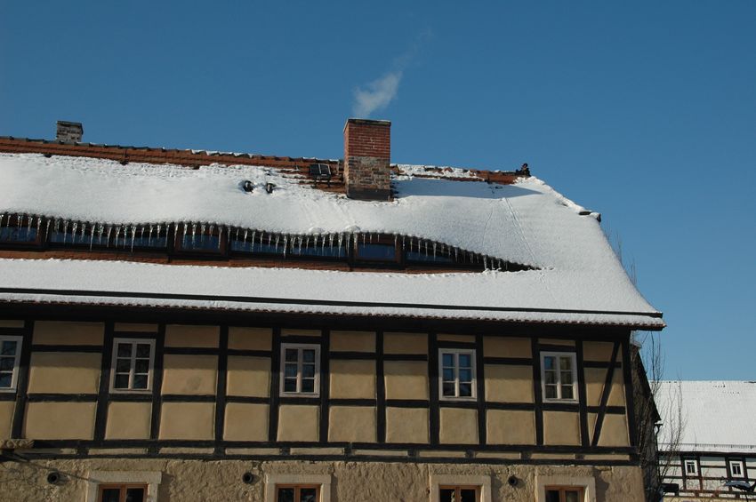
Figure 3. Percentage of correctly determined CFA pattern configurations after JPEG compression. Results for the green
channel configuration (left) and the complete RGB configuration (right). (‘∗’ refers to uncompressed images.)
5.2. Influence of the image size
Since our block-based algorithm decides with a majority rule, we expect the number of 2 × 2 blocks that are
taken into account to affect the reliability of the selection. The more blocks can be analyzed the more robust
becomes the decision. This is also supported by Tab. 3 that reports the percentage of correctly identified CFA
pattern configurations over all non-overlapping sub-images (i.e., blocks) of all never-compressed images in our
database. The block sizes were set to 256 × 256, 512 × 512 and 1024 × 1024, respectively. Observe how the
reliability increases with increasing image size, where the effect is more pronounced for the Adobe Lightroom
images. While the analysis of dcraw images (demosaiced with AHD) yields satisfactory results for a size of
256 × 256, the inspection of Lightroom images exceedingly benefits from larger dimensions. We can only suspect
that Lightroom applies some highly adaptive local processing, which is of course not without consequences on
our simple detector.
5.3. Influence of JPEG compression
No doubt, lossy JPEG compression is one of the most relevant forms of post-processing in our setting. Typ-
ical camera images are stored in this format, and a forensic method is generally desired to be—at least to
some extent—robust to JPEG post-compression. To explore the performance of our CFA synthesis approach
under lossy compression, we converted the demosaiced images in our test database to the JPEG format using
ImageMagick’s convert. JPEG qualities in the range {100, 98, 95, 90, 80} were used throughout our tests.
Figure 3 reports the percentage of correctly identified CFA pattern configurations after JPEG compression.
The left graph shows results for the green channel configuration, whereas results for the complete RGB con-
figuration are depicted on the right. As to be expected, the reliability drops with decreasing JPEG quality,
as quantization smooths out the subtle traces we are looking for. The performance decrease is however more
severe in the determination of the complete CFA configuration. Except for bilinear CFA interpolation, JPEG
qualities below 98 render a reliable identification impossible. The green channel configuration is generally better
identifiable. Here, only the analysis of VNG interpolated images suffers from a considerable performance loss.
Since all cameras listed in Tab. 1 are able to generate RAW images and JPEG images at the same time, we
can also use genuine JPEG images for our tests while keeping the general content of the test database constant.
Table 4 summarizes the results for camera JPEGs in the already known manner. It has to be mentioned that
JPEGs from the Nikon D70(s) are of lower quality, since, for performance reasons, the camera does not allow
high-quality JPEGs in the hybrid RAW/JPEG mode. Generally, the table gives a similar picture as with the
previous JPEG experiments. The valid green channel configuration is identifiable with high reliability, whereasthe performance for the complete configuration lags behind. Apart from the lower rates for the Nikon D70(s)
images (due to stronger JPEG compression), the absolute failure for the Nikon D200 images calls for particular
attention. Unfortunately, we are not able to provide a sound explanation of this behavior. On a technical level,
the semi-professional Nikon D200 is expected to produce JPEGs of very high quality. Furthermore, the cross-
correlation procedure described in the beginning of this section did not reveal any conspicuous deviation from
the uncompressed images. It is therefore a subject to future research to clarify this anomaly in a satisfactory
manner.
5.4. Influence of non-linear post-processing
In our last experiment we test for the influence of non-linear post-processing in terms of gamma correction. More
specifically, we processed all never-compressed images in our database according to the pixel-wise transformation
ỹi = (yi )γ , with γ ∈ {0.5, 0.6, . . . , 1.4, 1.5}. Since our CFA synthesis approach relies on a linearity assumption,
it could be expected that such non-linear post-processing hampers a correct identification of the CFA pattern
configuration. However, we found our method to be invariant to this particular type of non-linear processing
throughout the full range of all tested γ-values. Because the percentage of correctly identified configurations
more or less remained the same, we refrain from reporting them separately.
6. CONCLUDING REMARKS
We have presented an efficient method to determine the configuration of the color filter array (CFA) pattern in
demosaiced digital images. Derived from approximate solutions to the CFA synthesis problem,17 our approach
essentially requires only one linear filtering operation. Besides applications in the forensic analysis of digital
images, we believe that our method can also assist in related fields of multimedia security. Knowledge of the
pre-processing history of digital images as well as the structure of local inter-pixel correlation pattern can be
valuable both in steganography/steganalysis and digital watermarking.
While our method inherently assumes a linear demosaicing algorithm, it was demonstrated to reliably find the
correct CFA configuration in never-compressed images even for rather complex, signal-adaptive CFA interpolation
procedures. It will be nevertheless a subject to future research to investigate how similar efficient algorithms
can be found under more sophisticated demosaicing assumptions. One possible way to mimic signal-adaptive
interpolation algorithms lies in the derivation of specific approximate filters for regions with distinct horizontal
or vertical edges.
To a large part, the promising results obtained with our method can be attributed to the combined two-
stage block-based procedure. By first deciding on possible green channel configurations, the likelihood of finally
determining the complete RGB pattern configuration increases considerably. We found this observation to also
hold for other approaches with similar objectives. The analysis of small sub-blocks instead of the overall image
attenuates the effects of large local error terms (due to simplifying model assumptions), that can otherwise
accumulate to misclassifications. In our future work, we will explore the influence of the size of these blocks
which, in reference to the structure of the Bayer grid, was fixed to 2 × 2 in the course of this paper.
As to the limitations of our method we have to note that, not surprisingly, JPEG compression can severely
hamper a correct identification of the CFA pattern configuration. Here, it needs however to be distinguished
between the green channel and the complete RGB configuration. While the former is generally well identifiable
even under relatively strong compression, the latter requires a JPEG quality of 98 or higher. This surely calls
for further refinements to our method, for instance by applying more realistic demosaicing assumptions.
We finish this paper by returning to the very first basic assumption that was made, namely that the color
filter array has a Bayer pattern. In practice, of course, we cannot know whether this assumption is fulfilled,
and our method (together with other approaches that make similar assumptions) will not explicitly fail, when
it is not. Even though we believe that it is generally possible to extend the CFA synthesis procedure to other
layouts, there might always be a remaining source of uncertainty whether the very basic assumption is met. As
already pointed out by Swaminathan et al.4 in a similar context, it is thus of particular interest to derive some
type of a confidence score to weigh and evaluate the actual decision. On a more general level, we see endeavors
to develop detectors that can also opt for a neutral decision as a promising and practically relevant objective for
future research throughout the whole field of digital image forensics.ACKNOWLEDGMENTS
The author gratefully receives a doctorate scholarship from Deutsche Telekom Stiftung, Bonn, Germany.
APPENDIX A. APPROXIMATE CFA SYNTHESIS FILTER KERNELS
In Ref. 17, we showed that the general OLS minimization in Eq. (7) can be well approximated by linear filtering
with a fixed filter kernel. For the red and blue channel the kernels have the following numerical configuration:
∗ ∗ ∗ ∗ ∗ ∗ ∗ −0.001 ∗ ∗ ∗ ∗ ∗ ∗ ∗
∗ ∗ ∗ ∗ ∗ ∗ −0.001 −0.003 −0.001 ∗ ∗ ∗ ∗ ∗ ∗
∗ ∗ ∗ ∗ ∗ −0.001 0.003 0.006 0.003 −0.001 ∗ ∗ ∗ ∗ ∗
∗ ∗ ∗ ∗ −0.001 −0.003 0.006 0.015 0.006 −0.003 −0.001 ∗ ∗ ∗ ∗
∗ ∗ ∗ −0.001 0.003 0.006 −0.015 −0.036 −0.015 0.006 0.003 −0.001 ∗ ∗ ∗
∗ ∗ −0.001 −0.003 0.006 0.015 −0.036 −0.086 −0.036 0.015 0.006 −0.003 −0.001 ∗ ∗
∗ −0.001 0.003 0.006 −0.015 −0.036 0.086 0.207 0.086 −0.036 −0.015 0.006 0.003 −0.001 ∗
−0.001 −0.003 0.006 0.015 −0.036 −0.086 0.207 0.500 0.207 −0.086 −0.036 0.015 0.006 −0.003 −0.001
∗ −0.001 0.003 0.006 −0.015 −0.036 0.086 0.207 0.086 −0.036 −0.015 0.006 0.003 −0.001 ∗
∗ ∗ −0.001 −0.003 0.006 0.015 −0.036 −0.086 −0.036 0.015 0.006 −0.003 −0.001 ∗ ∗
∗ ∗ ∗ −0.001 0.003 0.006 −0.015 −0.036 −0.015 0.006 0.003 −0.001 ∗ ∗ ∗
∗ ∗ ∗ ∗ −0.001 −0.003 0.006 0.015 0.006 −0.003 −0.001 ∗ ∗ ∗ ∗
∗ ∗ ∗ ∗ ∗ −0.001 0.003 0.006 0.003 −0.001 ∗ ∗ ∗ ∗ ∗
∗ ∗ ∗ ∗ ∗ ∗ −0.001 −0.003 −0.001 ∗ ∗ ∗ ∗ ∗ ∗
∗ ∗ ∗ ∗ ∗ ∗ ∗ −0.001 ∗ ∗ ∗ ∗ ∗ ∗ ∗
For the green channel the kernel has the following numerical configuration:
∗ ∗ −0.001 0.001 0.001 0.001 −0.001 ∗ ∗
∗ −0.001 0.003 0.005 −0.004 0.005 0.003 −0.001 ∗
−0.001 0.003 0.009 −0.022 −0.029 −0.022 0.009 0.003 −0.001
0.001 0.005 −0.022 −0.072 0.165 −0.072 −0.022 0.005 0.001
0.001 −0.004 −0.029 0.165 0.835 0.165 −0.029 −0.004 0.001
0.001 0.005 −0.022 −0.072 0.165 −0.072 −0.022 0.005 0.001
−0.001 0.003 0.009 −0.022 −0.029 −0.022 0.009 0.003 −0.001
∗ −0.001 0.003 0.005 −0.004 0.005 0.003 −0.001 ∗
∗ ∗ −0.001 0.001 0.001 0.001 −0.001 ∗ ∗
(A ‘∗’ denotes filter coefficients with absolute values < 10−3 .)
REFERENCES
1. H. T. Sencar and N. Memon, “Overview of state-of-the-art in digital image forensics,” in Algorithms, Archi-
tectures and Information Systems Security, B. B. Bhattacharya, S. Sur-Kolay, S. C. Nandy, and A. Bagchi,
eds., Statistical Science and Interdisciplinary Research 3, ch. 15, pp. 325–348, World Scientific Press, 2008.
2. H. Farid, “Image forgery detection,” IEEE Signal Processing Magazine 26(2), pp. 16–25, 2009.
3. A. C. Popescu and H. Farid, “Exposing digital forgeries in color filter array interpolated images,” IEEE
Transactions on Signal Processing 53(10), pp. 3948–3959, 2005.
4. A. Swaminathan, M. Wu, and K. J. R. Liu, “Nonintrusive component forensics of visual sensors using output
images,” IEEE Transactions on Information Forensics and Security 2(1), pp. 91–106, 2007.
5. A. E. Dirik, S. Bayram, H. T. Sencar, and N. D. Memon, “New features to identify computer generated
images,” in Proceedings of the 2007 IEEE International Conference on Image Processing (ICIP 2007), 4,
pp. IV–433–IV–436, 2007.
6. S. Bayram, H. T. Sencar, and N. Memon, “Classification of digital camera-models based on demosaicing
artifacts,” Digital Investigation 5, pp. 46–59, 2008.
7. Y. Huang and Y. Long, “Demosaicking recognition with applications in digital photo authentication based
on a quadratic pixel correlation model,” in Proceedings of the 2008 IEEE Conference on Computer Vision
and Pattern Recognition (CVPR 2008), 2008.8. A. C. Gallagher and T.-H. Chen, “Image authentication by detecting traces of demosaicing,” in IEEE
Workitorial on Vision of the Unseen (in conjunction with CVPR), 2008.
9. C. McKay, A. Swaminathan, H. Gou, and M. Wu, “Image acquisition forensics: Forensic analysis to identify
imaging source,” in Proceedings of the 2008 IEEE International Conference on Acoustics, Speech, and Signal
Processing (ICASSP 2008), pp. 1657–1660, 2008.
10. B. Wang, X. Kong, and X. You, “Source camera identification using support vector machines,” in Advances
in Digital Forensics V, G. Peterson and S. Shenoi, eds., IFIP Advances in Information and Communication
Technology 306, pp. 107–118, Springer Boston, 2009.
11. N. Fan, C. Jin, and Y. Huang, “A pixel-based digital photo authentication framework via demosaicking inter-
pixel correlation,” in MM&Sec’09, Proceedings of the Multimedia and Security Workshop 2009, September
7-8, 2009, Princeton, NJ, USA, pp. 125–130, ACM Press, (New York, NY, USA), 2009.
12. A. E. Dirik and N. Memon, “Image tamper detection based on demosaicing artifacts,” in Proceedings of the
2009 IEEE International Conference on Image Processing (ICIP 2009), 2009.
13. H. Cao and A. C. Kot, “Accurate detection of demosaicing regularity for digital image forensics,” IEEE
Transactions on Information Forensics and Security 4(4), pp. 899–910, 2009.
14. R. Böhme, F. Freiling, T. Gloe, and M. Kirchner, “Multimedia forensics is not computer forensics,” in
Computational Forensics, Third International Workshop, IWCF 2009, The Hague, Netherlands, August
2009, Proceedings, Z. J. Geradts, K. Y. Franke, and C. J. Veenman, eds., Lecture Notes in Computer
Science LNCS 5718, pp. 90–103, Springer Verlag, (Berlin, Heidelberg), 2009.
15. J. Fridrich, Steganography in Digital Media: Principles, Algorithms, and Applications, Cambridge University
Press, 2009.
16. P. Meerwald and A. Uhl, “Additive spread-spectrum watermark detection in demosaicked images,” in
MM&Sec’09, Proceedings of the Multimedia and Security Workshop 2009, September 7-8, 2009, Prince-
ton, NJ, USA, pp. 25–32, 2009.
17. M. Kirchner and R. Böhme, “Synthesis of color filter array pattern in digital images,” in Proceedings of
SPIE-IS&T Electronic Imaging: Media Forensics and Security, E. J. Delp, J. Dittmann, N. D. Memon, and
P. W. Wong, eds., 7254, 72540K, 2009.
18. M. Kirchner and R. Böhme, “Hiding traces of resampling in digital images,” IEEE Transactions on Infor-
mation Forensics and Security 3(4), pp. 582–592, 2008.
19. G. C. Holst and T. S. Lomheim, CMOS/CCD Sensors and Camera Systems, SPIE Press, 2007.
20. R. Ramanath, W. E. Snyder, Y. Yoo, and M. S. Drew, “Color image processing pipeline,” IEEE Signal
Processing Magazine 22(1), pp. 34–43, 2005.
21. B. E. Bayer, “Color imaging array.” US Patent, 3 971 065, 1976.
22. S. Van Huffel and J. Vandewalle, The Total Least Squares Problem: Computational Aspects and Analysis,
vol. 9 of Frontiers in Applied Mathematics, Society for Industrial and Applied Mathematics, 1991.
23. Y. Huang and W. McColl, “Analytical inversion of general tridiagonal matrices,” Journal of Physics A:
Mathematical and General 30, pp. 7919–7933, 1997.
24. G. H. Golub and C. F. van Loan, Matrix Computations, Johns Hopkins University Press, 1996.
25. T. Gloe and R. Böhme, “The Dresden Image Database for benchmarking digital image forensics,” in Pro-
ceedings of the 25th Symposium on Applied Computing (ACM SAC 2010), pp. 1585–1591, 2010.
26. E. Chang, S. Cheung, and D. Y. Pan, “Color filter array recovery using a threshold-based variable number
of gradients,” in Proceedings of SPIE-IS&T Electronic Imaging: Sensors, Cameras, and Applications for
Digital Photography, N. Sampat and T. Yeh, eds., 3650, pp. 36–43, 1999.
27. K. Hirakawa and T. W. Parks, “Adaptive homogeneity-directed demosaicing algorithm,” IEEE Transactions
on Image Processing 14(3), pp. 360–369, 2005.You can also read