EARTH-IMPACT PROBABILITY COMPUTATION OF DISRUPTED ASTEROID FRAGMENTS USING GMAT/STK/CODES
←
→
Page content transcription
If your browser does not render page correctly, please read the page content below
AAS 11-408
EARTH-IMPACT PROBABILITY COMPUTATION OF DISRUPTED
ASTEROID FRAGMENTS USING GMAT/STK/CODES
Alan Pitz,∗ Christopher Teubert,∗ and Bong Wie†
There is a nationally growing interest in the use of a high-energy nuclear dis-
ruption/fragmentation option for mitigating the most probable impact threat of
near-Earth objects (NEOs) with a short warning time. Consequently, this paper
investigates the orbital dispersion and impact probability computation problem
of a disrupted/fragmented NEO using several computer programs, called General
Mission Analysis Tool (GMAT) developed by NASA, AGI’s Satellite Tool Kit
(STK), and Jim Baer’s Comet/asteroid Orbit Determination and Ephemeris Soft-
ware (CODES). These tools allow precision orbital simulation studies of many
fragmented bodies, with high-fidelity visualizations. Various mathematical mod-
els for impact probability computation are examined and compared to JPL’s Sen-
try, which is a highly automated NEO collision monitoring system. For example,
we obtained an impact probability of 4.2E-6 for asteroid Apophis on April 13,
2036, which is very close to 4.3E-6 predicted by JPL’s Sentry system. Our re-
search effort of exploiting various commercial software such as GMAT, STK, and
CODES will result in a robust software system for assessing the consequence of
a high-energy nuclear disruption mission for mitigating the impact threat of haz-
ardous NEOs.
INTRODUCTION
Asteroids and comets have collided with the Earth in the past and are predicted to do so in
the future. These collisions have a significant role in shaping Earth’s biological and geological
history, most notably the extinction of the dinosaurs 65 million years ago. Another event is the 1908
Tunguska impact in Siberia, which released an explosion energy equivalent to approximately five
to seven megatons of TNT. This explosion had enough power to destroy a 25 km radius of forest.
It has been estimated that an impact from the asteroid 99942 Apophis would release approximately
900 megatons of energy, over 130 times the Tunguska event.1 The results of a collision of this
magnitude in a highly populated area would be catastrophic.
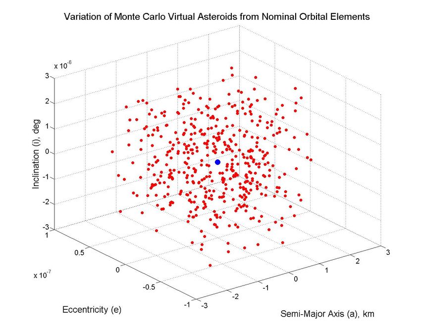
This paper is the first step of developing an interface that combines the research efforts in the As-
teroid Deflection Research Center with high-fidelity commercial software. The interface is called
the Asteroid Mission Design Software Toolbox (AMiDST) to be used for validating and enhancing
research in computational astrodynamics using Graphics Processing Units (GPUs), Yarkovsky ef-
fect modeling, GN&C algorithms, and nuclear fragmentation modeling. These core research areas
will connect through the use of the AMiDST which utilizes JPL’s Horizons, CODES, GMAT, STK
along with AGI Components, MATLAB, and GMV’s CLEON software as illustrated in Figure 1.
∗
Research Assistant, Asteroid Deflection Research Center, Iowa State University, 2271 Howe Hall, Room 2355, Ames, IA
50011-2271, alanpitz@gmail.com, teubert@iastate.edu.
†
Vance Coffman Endowed Chair Professor, Asteroid Deflection Research Center, 2271 Howe Hall, Room 2355, Ames,
IA,50011-2271, bongwie@iastate.edu.
1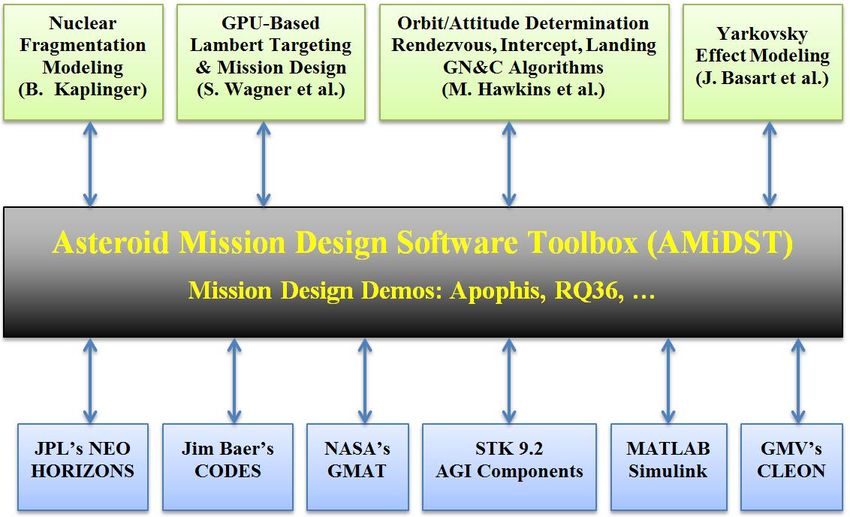
The AMiDST is being developed to be used for the design and analysis of real deflection/disruption
missions in the future, which will require reliable, high-fidelity, precision orbital modeling and sim-
ulations. The commercial software toolbox incorporates all aspects of the mission and creates a
foundation for innovation and validation of asteroid missions. Figure 1 depicts the overall research
goal while this paper is the first step of developing the AMiDST.

         Figure 1. Illustration of the Asteroid Mission Design Software Toolbox (AMiDST).

   Given short warning times, high-energy disruption missions, such as delivering a nuclear explo-
sive device to an asteroid, are needed to properly disperse the asteroid fragments from hitting the
Earth.2 Orbital dispersion simulation and analysis results show that fragmenting and dispersing a
hazardous NEO could lower the total mass impacting the Earth.3 This could be beneficial in sit-
uations where some impacting mass is inevitable, or where the resulting fragments will be small
enough to burn up in Earth’s atmosphere.2 Having an impact probability assessment of such a
disruption mission will prove whether Earth is safe from multiple fragments. This paper presents
software validation, trajectory analysis, and the implementation of Monte Carlo simulations to find
the impact probability of a hazardous NEO. The tools used to find the impact probability can be eas-
ily modified to study the consequences of disrupted asteroid fragments from high-energy nuclear
disruption missions of Earth-threatening bodies, with short warning time. To accurately estimate
the impact probability of disrupted asteroid fragments, commercial mission analysis software are
utilized, which include NASA’s General Mission Analysis Tool (GMAT), AGI’s Satellite Tool Kit
(STK), Jim Baer’s Comet/asteroid Orbit Determination and Ephemeris Software (CODES), and
JPL’s Horizons.
  There has been a great deal of discussion over the probable impact threat posed by the asteroid
Apophis. This possible threat makes Apophis an ideal reference model to study. On April 13,
2029, the asteroid Apophis will have a close-encounter with Earth, in which the asteroid will pass

                                                  2
below geostationary orbit.4 Apophis could pass through a keyhole and impact the Earth on April
13th, 2036. Keyholes are very small regions of the first encounter target-plane causing a resonant
return impact with the Earth if an NEO passes through it.4 Due to the uncertainty in observations,
gravitational effects, and other forces, orbit trajectories of small bodies are very difficult to predict
in long-term periods. The impact probability of Apophis in 2036 is currently estimated as four in
one million, according to JPL’s Sentry system.1
   Apophis was first discovered in 2004. Tables 1 and 2 show the physical parameters and orbital
elements respectively of Apophis from JPL’s Apophis orbit solution #144. Throughout this study,
Apophis is used as a reference asteroid and these orbital elements are used in each simulation. The
overall research objective is met but with much difficulty due to the nature of the problem, the
software inflexibility, and orbit differences in each software. These differences have been noted and
documented, but further investigation of these differences is required.

Table 1. Physical Parameters of Apophis taken           Table 2. Orbital elements of Apophis at Epoch
from JPL.1                                              2455800.5 (2011-Aug-27.0) TDB.1
        Physical Parameters       Value                        Orbital Elements         Value
        Rotational Period (hrs)   30.5                         Semi-Major Axis (AU)     0.92230
        Mass (kg)                 4.5E10                       Eccentricity             0.19108
        Diameter (m)              270                          Inclination (deg)        3.3319
        Absolute Magnitude H      19.7                         Ω (deg)                  204.4304
        Albedo                    0.33                         ω (deg)                  126.4245
                                                               Mo (deg)                 287.5823

TRAJECTORY ANALYSIS OF APOPHIS USING STK/GMAT/CODES
Introduction
   STK is a graphical user interface software for modeling and analyzing several applications in-
cluding flight paths and logistics, communications, satellites in specific orbits, Earth satellites, de-
fense applications, and more.5 With high-fidelity visualizations, STK has a multitude of features
that trump most physics-based computer programs. A communication interface between STK and
MATLAB can be established to utilize functions and script files created in MATLAB while exploit-
ing STK features such as propagators, orbit properties, and post-processing components. Propa-
gators that manage interplanetary missions include the High Precision Orbit Propagator (HPOP)
and Astrogator.5 Astrogator is a highly-versatile component of STK used to study detailed mission
scenarios, including the detailed parameterization of the spacecraft subsystems (dry and wet mass,
mass flow rates, pressures of fuel tanks, etc.). The high-fidelity visualization that STK provides for
conceptual mission design is invaluable to space applications.5
  GMAT is a space trajectory optimization and mission analysis software developed by NASA,
the space community, and the open source community. GMAT’s primary goal is to “research, de-
velop, verify, and transfer new technologies in space trajectory optimization and mission design.”7
GMAT is completely open-source allowing for user extension and personalization. MATLAB, min-
imization, and optimization plug-ins have been released and developers are currently working on a
plug-in between GMAT and the MATLAB Orbital Dynamics Toolbox. A built-in scripting language
included with GMAT allows for mission creation and modification. The user is able to create their
own propagators from a list of integrators and force models. GMAT contains a new but powerful

                                                   3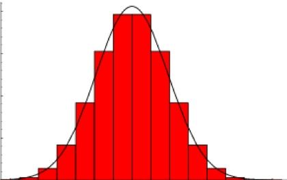
visualization tool for modeling and analyzing mission concepts with emphasis on space missions
around Earth or in the Solar System. The Mac and Linux releases of GMAT 2011a are currently in
the Alpha stage in the design process while the Windows release is in the Beta.
   CODES is a graphical user interface program written by Jim Baer. CODES calculates a variety
of small body characteristics such as orbits, optical observations, and physical parameters using a
precise n-body numerical integrator. It can use topocentric or geocentric ephemeris based on user-
specification or import minor bodies from the Minor Planet Center (MPC) database.8 Additionally,
it allows for linear and non-linear analysis of collisions/near misses between minor planets and
major planets. Calculation of the state vector or orbital elements with covariance matrices can be
obtained using an n-body simulator accounting for solar radiation pressure, gravity harmonics, and
relativistic effects.
   JPL’s Solar System Dynamics Group provides an on-line ephemeris computation service that
provides flexible information about solar system objects. JPL’s Horizons has three different ac-
cess methods; telnet, e-mail, and web-browser. The web interface provides access to a small sub-
set of program functions with an interactive GUI.9 The system provides access to highly accurate
ephemerides for solar system objects including over 560,000+ asteroids and comets, 9 planets, the
sun, natural satellites, spacecraft, and more.9,10 Close-approaches by asteroids and comets to the
planets, Ceres, Pallas, and Vesta, can be identified along with the encounter uncertainties and im-
pact probabilities. Orbital uncertainties and covariance matrices can be computed for asteroids and
comets. The underlying planet/satellite ephemerides and small-body osculating elements are the
same ones used at JPL for radar astronomy, mission planning and spacecraft navigation.9

Apophis Orbit Simulation Using STK 9.2
   In STK, the HPOP is used to propagate interplanetary trajectories with a solar radiation pressure
model, user-specified selection of third-body gravity, object rotation, and high-fidelity visualiza-
tions. The HPOP can use several different integrators for numerical analysis. The default integrator
for HPOP is the Runge-Kutta-Felhberg (RKF) of order 8 to estimate the local error in the method
of order 7. The RKF 7(8) is an integration technique utilizing polynomial functions to approximate
the ordinary differential equations.11 The RKF 7(8) has a variable step size for integration. If the
difference between two solutions is outside the bounds of the error tolerance, set by the user, then
the solution is estimated again with a decreased step size.11 Another type of integration scheme that
employs a variable step size is the Gragg-Bulirsch-Stoer (GBS) method. This method utilizes ratio-
nal functions as fitting functions for the Richardson extrapolation instead of polynomial functions.12
It is also combined with a modified midpoint method which is extremely important in the accuracy
of the solution. This method also has a variable step size. Lastly, a Gauss-Jackson (GJ) integra-
tion scheme is used to propagate an orbit. The Gauss-Jackson fixed, multi-step predictor-corrector
method is widely accepted in numerical integration problems for astrodynamics.13
   The default minimum and maximum step sizes for both the RKF and the GBS integrator are
1 second and 86400 seconds, respectively. The default error tolerance is 1.0E-13. A change to
these default values is listed in Table 3. In order to compare STK to other commercial software, a
reasonable compromise was reached for the minimum and maximum step size and error tolerance.
For planetary flyby sequences, a minimum step size is most likely used due to the large gravity
terms acting on the body. An average speed of an asteroid around the sun is approximately 30 km/s.
If the default minimum step size of 1 second is chosen, the distance traveled during one time step
is 30 km. Thus if a minimum step size is used during these times, a propagation of 3 meters per

                                                  4
step is sufficient. When studying the effects of Earth’s gravity on a small asteroid body, a rigorous
selection of a step size is important and a 1 second step size is not acceptable. These values listed
in the table are used throughout all the STK test cases in this study.
Table 3. Integration parameters in STK 9.2.
Integration Method Minimum Step-Size (Sec.) Maximum Step-Size (Sec.) Error Tolerance
RKF 0.0001 15,000 1.0E-11
GBS
GJ 15,000 N/A N/A
The solar radiation pressure model was included based on Apophis’s physical parameters such
as the slope parameter, albedo, spin rate, size, and mass. The solar radiation pressure model is
assumed to be a spherical model with properties reflecting those shown in Table 1. Third-body
gravity includes all 9 planets and Earth’s moon from ephemeris file DE-421. The Yarkovsky model
and relativistic effects were not included in this study.
A comparison is made against the three different integration methods with the same force models.
The epoch position and velocity is chosen from JPL’s Horizons on January 1, 2029 in the J2000
Ecliptic Coordinate System. STK then propagated the object multiple times, each with a different
integration method. The differences are calculated against one another and the results are shown
in Table 4. Based on the propagation prior to the close-approach with Earth, it was found that all
integrators are able to produce exactly the same results. However one and one-half month later, the
Gauss-Jackson integration scheme fails completely due to its fixed step size. If a smaller window of
time is to be analyzed with an extremely small step-size, a Gauss-Jackson integrator is as reliable
as the other integrators. Since the study of the asteroid is much more than two months, a Gauss-
Jackson is not used. Also, from the differences, the Gragg-Bulirsch-Stoer method is nearly identical
to the RKF 7(8). This is important in comparing the other mission analysis software since both
GMAT and STK have the Gragg-Bulirsch-Stoer method but not the same RKF order method. Due
to excessively long computation time, the Gauss-Jackson fixed step-size is not further reduced.
Table 4. Difference between integration schemes in STK at Epoch of January 1, 2029 from Horizons.
Date X (km) Y (km) Z (km) Ẋ (m/s) Ẏ (m/s) Ż (m/s)
1-Mar-29 0 0 0 0 0 0
RKF - GBS 13-Apr-29 9.95E-2 2.67E-2 2.21E-2 1.20E-2 2.0E-3 2.0E-3
1-Jun-29 0.20 6.84E-4 7.94E-2 0 0 0
1-Mar-29 0 0 0 0 0 0
RKF - GJ 13-Apr-29 5.77E-2 1.02E-2 1.14E-2 7.00E-3 1.00E-3 1.00E-3
1-Jun-29 3.63E+6 1.16E+6 5.51E+5 838.12 642.39 81.16
1-Mar-29 0 0 0 0 0 0
GBS - GJ 13-Apr-29 0.16 3.69E-2 3.35E-2 1.90E-2 3.00E-3 3.00E-3
1-Jun-29 3.63E+6 1.16E+6 5.51E+5 838.12 642.39 81.16
5Apophis Orbit Simulation Using GMAT
GMAT’s main strength over other software choices is its versatility. Its scripting ability is easy
to use and edit without any knowledge of computer languages. The MATLAB plug-in allows an
expansion of the user’s ability to personalize each mission. Rather than choosing from a list of
possible propagators, the user is able to create his/her own by choosing the propagation settings
such as integrator scheme, step size, error tolerance as well as the gravitational bodies, and the
non-gravitational forces including drag, solar radiation pressure, and more.
In GMAT there are seven different n-body numerical integrators to choose from. These include
the Runge-Kutta 5(6), Runge-Kutta 6(8), Runge-Kutta 8(9), Prince-Dormand 4(5), Prince-Dormand
7(8), Bulirsch-Stoer, and the Adams-Bashforth-Moulton method. Each of these integrators employ
variable step sizes and are well tested by the GMAT team. The Runge-Kutta (RK) method, as
explained earlier, is a single-step method employing a series of coupled variables to solve differen-
tial equations.14 The Prince-Dormand (PD) method as used in PD 78 and PD 45 is a form of an
expanded RK method.
Unfortunately, the Bulirsch-Stoer method could not complete the propagation test within the ac-
curacy limit for long periods of time (more than 7 years). Therefore, this method is considered
only as a verification tool but was not used for impact probability simulations. Adams-Bashforth-
Moulton, on the other hand is an implicit linear multistep method that iteratively solves the differ-
ential equation. The Adams-Moulton integration method is used as a differential corrector for the
Adams-Bashforth integration allowing for multistep integration.15 The Adams-Bashforth-Moulton
method also could not complete the propagation within the accuracy limit.
The propagation test comprised of using several different integrators each having the same step
sizes and error tolerances. The planetary bodies use ephemeris data from DE-405. Apophis solution
#144 is used as the starting conditions listed in Table 2. Each case propagated from August 2011
until April 13, 2036. The 2029 close-approach distance was found as well as the 2036 distance.
Table 5 shows the results of the integration test cases.
Each propagator’s nominal close-approach distance in 2029 and 2036 is compared to distinguish
which integrator performs best. After running each integrator, no difference was seen in the 2029
close-approach. However, after further review of STK and CODES, the Runge-Kutta 8(9) was
chosen as the default integrator for simulations. Additionally, after careful evaluation and testing, a
maximum step of 15,000 seconds, a minimum step of 1E-4 seconds, and an accuracy of 1E-11 were
chosen.
Table 5. Comparison of GMAT Integration Methods using Apophis.
Integration Method 2029 Distance, km 2036 Distance, km Runtime, sec
RK 89 37,344.48 20,323,355.5 88.92
RK 68 37,344.48 20,323,302.7 50.21
PD 78 37,344.48 20,323,313.9 70.44
Once the integration method is selected, integration parameters can be chosen for the initial step
size, accuracy limit, minimum step size, maximum step size, and maximum step attempts. Variable
step size calculations change the step size within the bounds set by the minimum and maximum step
size variables to achieve the given accuracy limit. If the accuracy is determined to be outside the
6acceptable range then the integration is repeated with a smaller step size. This is repeated until the
accuracy is obtained, the minimum step size is used, or the number of attempts equals the maximum
step attempts. If the accuracy cannot be reached, an error is displayed and the program stops. If the
accuracy is reached, the integrator moves onto the next step and repeats the process.
GMAT has several different options regarding which gravitational bodies the user wants. Grav-
itational bodies include the sun, 9 planets, Earth’s moon, several large asteroids, and 300 known
asteroids. After studying the effects of these bodies it was determined that including all the bodies
is not necessary. Many of the smaller bodies have such a small effect on the orbit of an asteroid
that they can be neglected. Taking out these bodies improves computation time allowing for more
simulations to be run.
For the reference asteroid Apophis, simulations including various heavenly bodies are run to
determine at what point their effect becomes negligible. After running these tests, which can be
seen in Table 6, the sun, 9 planets, Earth’s moon, Ceres, Vesta, Pallas are determined to be the
bodies with the largest influence on Apophis. Including other bodies increased the computation
time with no significant change in the close-approach distance. Ceres, Vesta and Pallas are added to
GMAT by importing their SPICE files, but all the other bodies came built-in with GMAT.
Table 6. Comparison of GMAT Results with Different Gravitational Bodies.
Sun, Earth, Sun, 9 Planets, Sun, 9 Planets,
Sun Only & moon moon, Ceres, & 300 Aster-
Vesta, & Pallas oids
2029 Distance, km 3,317,819 5,420,063 37,344.5 37,345.1
Runtime, sec 34.94 40.00 45.17 72.12
Another important gravitational force that must be considered for any accurate model is non-
spherical gravity. This is accounted for within the integration model with the use of .cof potential
files. Gravitational potential files for Venus, Earth, Earth’s moon and Mars are built into GMAT,
but it also allows for users to add other bodies manually. Repeated tests for the asteroid Apophis
revealed that only the Earth’s non-spherical gravity has a significant effect. This is possibly because
of the 2029 close-approach to the Earth. Future simulations will include Earth as a non-spherical
gravitational model.
Other non-gravitational forces can also be included in the propagation. Currently, these include
drag and solar radiation pressure (SRP), but the GMAT support team plans on expanding this to
include both relativistic and Yarkovsky effects. GMAT includes high-fidelity models, not only for
atmospheric drag but also F10.7 drag, and magnetic drag of the Earth. The SRP model can be
applied using the albedo, spin rate, size and mass of the asteroid. Both drag and SRP forces are
included in the Monte Carlo simulation described later.
Apophis Orbit Simulation Using CODES
CODES is a graphical user interface program used to calculate a variety of information using
observations, an N-body numerical integrator, and physical parameters. First, the program asks to
designate the type of object, whether it be an asteroid or comet. Afterwards, the user can import a
body from the Minor Planet Center (MPC), load in observations, or manually specify an orbit. If
observations are chosen the program allows evaluation of the observations and propagates the object
7with a best-fit orbit using n-body mechanics. These observations can then be compared to positions
of known minor planets.
One reason that makes CODES credible is the N-body numerical propagator and force models.
The N-body propagator has three options: include all 9 planets and Earth’s moon, or the 9 planets,
moon, plus Ceres, Pallas, and Vesta, or the 9 Planets, moon, and 300 asteroids.8 The planetary
bodies use ephemeris data from DE-405 while the 300 asteroids use BC-405. Having a rigorous
propagator increases computation time and accuracy. The force models include solar radiation
pressure, relativistic effects, and gravity harmonics. The numerical integrator utilizes a Dormand-
Prince embedded Runge-Kutta 7(8) method.
In this paper, the N-body propagator including the 9 planets, Earth’s moon, plus Ceres, Pallas,
and Vesta was used for CODES simulation runs. Once the orbit has been propagated, the user can
extract the heliocentric ecliptic J2000 orbital elements or state vector at epoch. The orbital elements
and state vector can also be propagated to a new epoch with a new covariance matrix. This is
important when trying to study an asteroid’s orbit further in the future without having to propagate
the state vector from the original epoch each time.
Lastly, the collision and/or near miss tool can be used to check for any collisions or near misses to
all major planets or Earth. The tool is broken down into a linear and nonlinear analysis. The linear
analysis propagates the nominal state vector and covariance matrix to the specified end date. Using
N-body mechanics and force models, CODES checks the distance between the object and distance
to a solar system body (Sun, planets, and Earth’s moon).8 If the calculated distance is under the
specified distance then a near miss is predicted. CODES uses the state vector and covariance matrix
to estimate the probability of collision. On the other hand, if the calculated distance is less than
the radius of the solar system body, then a collision has occurred and is reported. CODES uses a
bisection method that determines the exact date and time of the collision.8 All of these near misses
and collisions are reported in a text file at the end of the simulation.
The nonlinear analysis can also be used. The analysis is primarily used for multiple near misses
that result in sensitive orbit trajectories. A nonlinear analysis handles a user-specified number of
variant state vectors either distributed normally about the nominal epoch state vector or uniformly
along the Line-of-Variations (LOV).8 The LOV is the major axis of the epoch state vector uncer-
tainty ellipse. Once these state vectors are created, they are then propagated in the same manner as
the linear method. If a near miss is found, a Monte Carlo simulation model is created by introducing
virtual asteroids to extensively examine the close-approach distance and impact probability.
Unfortunately for our study, the nonlinear analysis, which is required to determine the impact
probability of a small body, is not currently setup to handle a specified or imported nominal state
vector. Instead, it is required to have both the observations and best-fit orbit with covariance matrix.
The nonlinear analysis involves adding normally distributed noise to each observation, calculating
the resulting orbit and then propagating it.
Using CODES with a specified orbit from Apophis solution #144 as listed in Table 2, a linear
collision analysis was ran. The n-body propagator was chosen as well as the physical parameters
were set as shown in Table 1. Table 7 shows the results of the linear analysis simulation. It accurately
depicts the close-approach in 2029 with a near miss of 5.97 Earth radii or 38,078 km. Due to the
linear analysis and the sensitivity of the close-approach distance in 2029, the near misses, past 2029,
should be checked using a nonlinear analysis. All the miss distances are represented in Earth radii.
The original intention of using CODES was to validate the impact probability estimation made
8Table 7. Collision/near miss results of a linear analysis for 50 years of Apophis with Epoch on August
27, 2011.
year mm dd hh mm secs Nominal Miss Distance (er) Impact Probability
2013 01 09 11 42 11.4 2,267.18 0.0
2021 03 06 01 13 43.7 2,642.21 0.0
2029 04 13 21 45 08.9 5.97 0.0
2036 03 26 05 37 38.6 7,859.87 0.0
2037 09 23 01 42 34.2 4,525.3 0.0
2044 07 31 02 52 16.3 2,585.68 0.0
by JPL’s Sentry. Once found, the next step is to study the effects of fragments, from a nuclear
disruption mission, with an impacting trajectory 15 days prior to impact Earth, and then run a
Monte Carlo simulation scenario of the impacting object to determine the impact probability of
having multiple fragments hit the Earth. However, due to the inflexibility of CODES, this type
of collision assessment cannot be accurately found using a specified orbit with covariance matrix.
Future upgrades for CODES, to name a few, include determination of impact on a planet using
latitude and longitude, additional asteroid perturbations, Yarkovsky effect, and implementation of
JPL’s DE-406 planetary ephemeris.
Comparison of Orbit Simulation Results for Apophis
Validation is the first priority to ensure reliable results from the mission analysis software. By
testing each software and their respective integrator/propagator using identical initial conditions,
validation is achieved. Each program is tested using the same position and velocity vector taken
from JPL’s Horizons in the J2000 Ecliptic Coordinate System using the same integrator, step size,
and error tolerance. Between STK and GMAT a variable step size Gragg-Bulirsch-Stoer integrator
scheme is used for propagation. The force models for each are also identical in nature including
the solar radiation pressure and third body gravity. JPL’s Horizons does not use the same integrator
scheme but an Adams-Krogh integrator, named DIVA, with a variable order and variable step size.10
It contains highly-accurate force and dynamical models used to provide conclusive ephemeris in-
formation. For small bodies, JPL’s Horizons uses integrated gravitational point-mass equations of
motion and can be extended to include solar radiation pressure, Yarkovsky effect, gravity harmon-
ics, and relativistic effects.10 Although GMAT, STK, and Horizons do not all share the common
propagator and properties, similarities can still be drawn among them.
After individual software propagation, the position and velocity vectors are recorded at predefined
times. These test cases assess each program’s ability to calculate Apophis’s close-encounter in 2029
for two months as well as deep-space propagation for several years. There are two types of cases
that are used to gather information. Case 1 focuses on the close-approach distance between the
asteroid and Earth. The case starts one month prior to the close-approach in 2029 and ends one
month after. Case 2 examines the deep-space propagation of the asteroid from one month after
the close-approach in 2029 until a possible impact on April 13, 2036. The positions and velocities
within each program are recorded and checked against JPL’s Horizons.16 Tables 8 and 9 show the
differences in the position and velocity vector components for each case at the specified date.
Case 1 starts with an epoch on March 13, 2029 using position and velocity vectors of Apophis
9from Horizons. This information is then entered into STK and GMAT. Once propagated, the posi-
tion and velocity vector on April 13 and May 13 of 2029 are recorded. These differences shown in
Tables 8 and 9 show differences between STK and Horizons and GMAT and Horizons. It should
be noted that both have a relatively large difference on May 13, however, the difference of both are
relatively of equal value. Thus, STK and GMAT match closely with one another for planetary close
flybys.
In Case 2, the difference between STK and Horizons is greatly significant and it should be noted
as an undesirable difference. Case 2 starts with an epoch date of May 13, 2029 with position and
velocity vectors taken from Horizons. After one year of deep-space propagation, the difference
between GMAT and Horizons is very small. This implies that the propagation results from GMAT
and Horizons are similar for deep space propagation but differ slightly in planetary close flybys.
On the other hand, the propagation results from STK and Horizons differ considerably on May 13,
2030. The error between them increases as the propagation continues. A difference of 33,000 km is
not acceptable for scientific purposes in the study of accurate impact probability computation.
Table 8. Case 1: Difference Between Horizons and STK/GMAT for Epoch of March 13, 2029.
Date X (km) Y (km) Z (km) Ẋ (m/s) Ẏ (m/s) Ż (m/s)
13-Apr-29 11.49 10.42 5.80 0.25 0.13 0.06
STK
13-May-29 69,138.30 213,142.12 91,981.88 16.01 85.53 32.55
13-Apr-29 20.98 6.03 5.29 0.28 0.12 0.06
GMAT
13-May-29 68,385.27 213,523.94 89,183.43 15.69 85.75 31.55
Table 9. Case 2: Difference Between Horizons and STK/GMAT for Epoch of May 13, 2029.
Date X (km) Y (km) Z (km) Ẋ (m/s) Ẏ (m/s) Ż (m/s)
13-May-30 771.03 4,610.49 175.21 0.76 0.06 0.01
STK 13-Apr-36 25,000.73 20,351.78 1,105.38 4.71 4.45 0.08
13-May-36 33,482.19 4,856.95 689.32 1.36 7.15 0.23
13-May-30 0.06 27.29 0.42 4.92E-3 1.55E-5 9.19E-5
GMAT 13-Apr-36 38.27 39.58 2.03 8.18E-3 1.16E-2 3.22E-4
13-May-36 52.03 4.37 0.89 2.06E-3 1.52E-2 5.46E-4
Figure 2 shows the radial position differences of Apophis with respect to Horizons using STK and
GMAT. STK uses the RK 7(8) method and GMAT uses the RK 8(9) method with identical minimum
and maximum step sizes and error tolerances. This comparison uses the same time period as Case
2 along with the same ephemeris data files, DE-421. It is worth noting that there is an increasing
sinusoidal difference between STK and GMAT with Horizons for long-term propagation. However,
STK shows a much earlier radial position difference which then increases dramatically. GMAT
follows a similar trend but with a much smaller difference amplitude for the same propagation time.
Further investigation of this propagation error in STK is conducted using different integrators,
variable step sizes, fixed step sizes, higher error tolerances, and planetary ephemeris files. The
maximum step size of the Gragg-Bulirsch-Stoer method, is set at 3,750 seconds, one-fourth of
the initial maximum step size and the new position vectors are recorded. The difference is taken
10Figure 2. Radial Position Differences of Apophis w.r.t. JPL’s Horizons.
from both the GBS methods using different maximum step sizes in STK. The result showed little
difference between the new and the old step sizes. Finally, the Gauss-Jackson method was also
used in Case 2 with a step size of 60 seconds. On May 13, 2030, the Gauss-Jackson method and
GMAT’s GBS method resulted in a larger difference than shown in Table 9. Solar radiation pressure
model was also turned off in both STK and GMAT. However, the resulting change was a 10-30
km difference from the original orbit in both software. These differences have been noted but
examination of the error between the two programs is still continuing. AGI headquarters has heard
these differences through customer support and an investigation has begun.
IMPACT PROBABILITY MODELING
Knowledge of an asteroid’s position comes from a series of visual, radar and Doppler obser-
vations. From these observations a nominal orbit and uncertainty ellipsoid is determined. The
uncertainty ellipsoid is the volume inside which the asteroid must exist. The target asteroid’s actual
position could be anywhere within the uncertainty ellipsoid but statistically it is likely to be at the
nominal location. Many methods use a series of Virtual Asteroids (VAs) to determine impacting
probabilities. Each VA represents one possible location and orbit of the target asteroid of interest.
One consequence of this positional uncertainty is long-term trajectory propagation error. A prob-
ability distribution can then be used to estimate the impact probability (IP) of an asteroid hitting a
major body. This impact probability value is important for determining the impact risk of an asteroid
to a major body.
Monte Carlo Method
The Monte Carlo (MC) method is widely used for determining impact probability. This method
randomly samples a pool of Virtual Asteroids (VAs) from the uncertainty ellipsoid. Since the defi-
nite position and orbit of the asteroid is not precisely known, each VA represents a possible position
and orbit where the asteroid could exist. Each VA has its own set of six orbital elements which
include the semi-major axis, eccentricity, inclination, longitude of the ascending node, argument of
11periapsis, and mean anomaly angle (a, e, i, Ω, ω, Mo ). The VAs are propagated until the end date
in which the final position is recorded. A statistical tool uses these recorded positions to determine
the probability of impact. The MC method, is widely used to simulate unknown, complex physical
models such as the orbits of small bodies in the Solar System.
Virtual Asteroid Generation and Propagation
The first step in determining the impact probability using the Monte Carlo method is to create the
VAs. A pool of random numbers lying within the interval [0,1] is generated for this purpose. Both
GMAT and STK have MATLAB plug-ins allowing for the user to use built-in MATLAB random
number generators.
The pool of 6∗N random numbers is used to sample N VAs from the six-dimensional uncertainty
space (a, e, i, Ω, ω, Mo ). Each orbital element is independently and randomly sampled from a
Gaussian distribution as shown in Figure 3.
Figure 3. Example of a Gaussian Distribution.
√
a = σa 2 erf−1 (2 ∗ RAND − 1) + µa
(1)
The Gaussian distribution of orbital elements is achieved by taking the inverse cumulative dis-
tribution function of the random number pool.17 The inverse cumulative distribution function, as
described by Equation 1, is a function of the mean, standard deviation, and the random number
sampled from the pool.
This results in the creation of one of the six orbital elements for a VA. Repeating the process five
more times defines a VA. Values closer to the mean are favored to create a Gaussian distribution in
the pool. This results in a mean and standard deviation equal to the values entered into the MC. In
this case the mean and standard deviation are equal to those from Apophis solution #144 as provided
in Table 10.1
A scatter plot of the virtual asteroids’ semi-major axis, eccentricity, and inclination for the
Apophis Monte Carlo simulation is provided in Figure 4. Each red dot represents one of the 1000
virtual asteroids created each having its own set of six orbital elements. Each axis shows the vari-
ance from the nominal values. The nominal VA is represented by a blue dot located at (0,0,0).
At this point there are some checks that can be done to prevent spurious data. The first of these is
a test of the random number generator. The easiest way to do this is to find the mean and standard
12Table 10. Orbital elements of Apophis at Epoch 2455800.5 (2011-Aug-27.0) TDB from Apophis Solu-
tion #144.1
Orbital Elements Mean Value (µ) Standard Deviation (σ)
Semi-Major Axis (AU) 0.922300 7.674E-9
Eccentricity 0.191076 3.6429E-8
Inclination (deg) 3.331960 1.5069E-6
Ω (deg) 204.43041 3.0196E-5
ω (deg) 126.42447 3.0819E-5
Mo (deg) 287.5823 3.0636E-5
deviation of all the random numbers generated. For a large pool, the mean and standard deviation
values should be approximately equal to 0.5 and 0.34134, respectively. In the case where these
values do not match, a new pool of random numbers is generated.
Another method to detect dubious data, is to compare the mean and standard deviation of all
the VA’s six orbital elements. In this case, they are compared with JPL’s Small Body Database
Apophis’s Orbital Elements.1 Having too few VAs results in a difference between the calculated
and compared mean and standard deviation values.
The pool of VAs are then propagated until they reach perigee in 2036. This is the closest point
to the Earth the VAs reach in 2036. Each VA’s Cartesian position at perigee is recorded for use in
post-processing. Post-processing for determining the impact probability begins once all positions
are recorded.
Post-processing
The simplest post-processing method is executed by dividing the number of VAs that hit the
Earth, also called Virtual Impactors (VIs), by the total number of VAs used in the calculation. The
main limitation of such a method is that the number of VAs required is roughly equal to the inverse
of the impact probability.18 For an asteroid with an impact probability of approximately 1.0E-6,
at least one million VAs would be needed in order to validate this claim. This is computationally
expensive and difficult to manage; thus, alternative methods have been developed in the literature
using an impact probability model of the form:
ZZZ
IP = PDF(x, y, z) dx dy dz (2)
V⊕
One such method of decreasing the necessary number of simulations is to use a statistical ap-
proximation. The first step in doing this is to find the three-dimensional probability density function
(PDF) of the asteroid’s close-approach-position. The impact probability of Apophis becomes the
integral of the PDF over the volume of the Earth as defined by Equation 2. This expression can then
13Figure 4. Semi-Major Axis - Eccentricity - Inclination Scatter Plot of VAs created by
a Monte Carlo Model.
be simplified by converting it to spherical coordinates, as follows:
Zr⊕
IP = PDF(r) dr = CDF(r⊕ ) − CDF(0) (3)
0
1 r⊕ − µ 0−µ
= erf √ − erf √ (4)
2 σ 2 σ 2
where CDF denotes the cumulative density function, µ is the mean distance from the Earth, σ is the
standard deviation of the perigee distances from the Earth, and r⊕ is the radius of the Earth.
This process results in a number between 0 and 1 corresponding to the probability of impact.
The MC method must be repeated with various pools of VAs to ensure accuracy. If the difference
between the IPs predicted from each run is outside an acceptable range, then this implies that a
larger pool of VAs is required. Having a larger pool of VAs increases computation time but results
in a more accurate impact prediction.
Impact Probability of Apophis
The most basic application of various software options is finding the asteroid’s nominal close-
approach distance to the Earth. This value corresponds to the most probable close-approach distance
and is of great use in determining how dangerous a potential impactor is to Earth. For Apophis, a
comparison of the close-approach distance is made by each software starting with the same initial
14conditions. The conditions are set to reflect Apophis solution #144 listed in Tables 1 and 2. Starting
in August 2011 and propagated to April 13, 2029, the minimum distance was found. Table 11 shows
the miss distance of Apophis on April 13, 2029 during its closest approach using JPL’s Small Body
Database, NEODyS-2, CODES, GMAT and STK. This distance is within geosynchronous orbital
altitude and, though it will not hit the Earth, it may pose a danger to Earth’s satellites prompting the
need for continuous observations.
NEODyS-2 presents information for near-Earth asteroids including orbital elements, physical pa-
rameters, a covariance matrix, and a risk table with a convenient Web-based interface. The risk table
is calculated using an original software called OrbFit with collaboration with NEODyS/CLOMON2
team and JPL’s Sentry team. NEODyS-2 is comparable and similar to JPL’s NEO website. NEODyS-
2 also includes close-approach tables, ephemeris files, observational data, and possible impact so-
lutions. Table 11 shows the close-approach distance of Apophis in 2029. Figure 5 shows the 2029
close-approach of Apophis generated by GMAT.
Table 11. Nominal Miss Distance of Apophis on April 13, 2029 and Impact Probability in 2036 calcu-
lated by each software.
JPL’s Sentry NEODyS-2 CODES GMAT STK
2029 Distance, km 38,067 38,342 38,078 37,859 49,211
Impact Probability 4.3E-6 4.3E-6 - 4.2E-6 -
Figure 5. Nominal Trajectory of Apophis with a Close Earth Flyby on April 13, 2029,
created by GMAT.
Another use of various software options is determining the impact probability for an asteroid.
This impact probability number is important for determining the danger that a specific asteroid poses
to Earth. The asteroid Apophis is used here for comparison. In 2036 there is a small chance that
Apophis will impact the Earth. This is dependent on the asteroid going through a small ‘keyhole’
during the 2029 close flyby. Passing through this keyhole results in a 7/5 orbital resonance causing
an impact seven years later on April 13, 2036.
15The MC simulation is written in GMAT’s scripting language. A pool of 6000 random numbers
is created using an Inverse Transform Sampling Pseudo-Random Number Generator. The random
number distribution is checked and found to have a mean equal to 0.5 and a standard deviation equal
to 0.34134. This confirms that the random numbers are evenly distributed.
The pool of 6000 random numbers were then turned into orbital elements creating 1000 VAs.
The distribution is confirmed to be equal to the values listed in Table 10.1 Each set of six orbital
elements is assigned to a VA, and the VA is propagated until the 2036 perigee condition. Each state
vector is recorded at perigee into a report file. The created report file is then imported into Excel
for post-processing. Using built-in Excel functions and Equations 3 and 4, the impact probability is
then computed. A comparison of computed impact probabilities from different sources is provided
in Table 11. It can be noticed that we obtained an impact probability of 4.2E-6 for asteroid Apophis
on April 13, 2036, which is very close to JPL’s impact probability value of 4.3E-6.
Impact Probability Concept as Applied to Disrupted Apophis Fragments
If an NEO on an Earth-impacting course can be detected with a mission lead time of at least sev-
eral years, the challenge becomes mitigating its threat. When the time to impact exceeds a decade,
the velocity perturbation needed to alter the orbit is small (≈ 2 cm/s).3 When the time to impact
is short, the necessary velocity change may become very large, and the use of a nuclear subsurface
explosion may become inevitable.3 A common concern for such a powerful nuclear option is the
risk that the deflection or disruption mission could result in fragmentation of the NEO, which could
rather substantially increase the damage upon its Earth impact. Therefore, it is important to develop
a computational tool to determine the impact probability of the disrupted fragments from a nuclear
subsurface disruption mission.
A conservative estimation of the impacting mass for a worst-case mission scenario with a lead
time of 15 days before impact is studied for a nuclear subsurface explosion with a shallow burial (<
5 m) for a test case of Apophis in Refs. 2 and 3. At detonation, the energy source region expands,
creating a shock that propagates through the body resulting in fragmentation and dispersal. The
mass-averaged speed of the fragments after 6 seconds was near 50 m/s with a peak near 30 m/s.2
As a result only 0.2% of the initial mass resulted in impacting the Earth if the explosion direction is
aligned along the inward or outward direction of the orbit, i.e., perpendicular to NEO’s orbital flight
direction.3 Such a sideways push is known to be optimal when a target NEO is in the last orbit before
the impact. Obviously, the impact mass can be further reduced by increasing the intercept-to-impact
time or by increasing the energy level of nuclear explosives (i.e., higher yields).3
A simulation of a nuclear disruption mission of a fictitious Earth-impacting Apophis trajectory
is considered. Furthermore, the impact probability of the orbital dispersal fragments from this
nuclear disruption mission 15 days before impact is extensively examined. Table 12 displays the
modified state vector of an Earth-impacting Apophis at an Epoch date of March 29, 2036 in the
J2000 Ecliptic Coordinate System. This sample test case is used as a reference which demonstrates
the development of the AMiDST.
Table 12. Modified State Vector of Apophis at Epoch of March 29, 2036, in a Collision Course with
Earth on April 13, 2036.
X (km) Y (km) Z (km) Ẋ (km/s) Ẏ (km/s) Ż (km/s)
-155,168,152.5446 -23,546,881.5797 -1,508,530.2557 9.7751 -28.1744 1.1376
16The fragmentation model consists of an impulsive velocity perturbation which is applied to each
fragment. Typically, velocity perturbations of fragments from disrupted asteroids are non-Gaussian
with a tail of high-velocity ejecta. However in this sample test case, the magnitude of the velocity
perturbations is assumed to form a Gaussian distribution sampled randomly, with a mean value
of 50 m/s and a standard deviation of 10 m/s. The velocity perturbation direction is sampled to
favor directions perpendicular to Apophis’s velocity vector. For simplicity, the velocity perturbation
directions are set in the spherical coordinate system, with the origin at the asteroid’s body and the x-
axis along the velocity vector. By using the same Gaussian Monte Carlo method, the right ascension
is sampled with a mean value and standard deviation of 90◦ and 45◦ , respectively. The declination
is then sampled between 0◦ and 360◦ , randomly. This process is repeated to create N fragments
each having a random velocity magnitude and direction.
STK and GMAT are used to carry out the calculations of this disruption model. STK was chosen
for the illustration of this study due to its superior visualization tools and Astrogator feature. Due
to the short time frame of this simulation and little deep space propagation, STK’s performance for
this simulation study is not affected by the discrepancies noted earlier.
A sample test case of delivering a nuclear explosive device (NED) to a fictitious Apophis impact
is simulated and the results are illustrated in Figures 6-9. The simulation starts with the interception
by a spacecraft carrying a NED to the threatening asteroid Apophis as depicted in Figure 6. The
spacecraft intercepts Apophis on March 29, 2036, 15 days before the fictitious impact with Earth on
April 13, 2036.
Figure 6. Nuclear Disruption Mission for the Fictitious Impact of Apophis on April 13, 2036.
A dispersion cloud of fragments is created to simulate the consequence of a nuclear disruption of
Apophis.2 This cloud is created by imposing a velocity perturbation individually on each fragment.
In this visual sequence of events only 50 fragments were considered. The resulting orbital dispersion
forms a debris cloud as shown in Figure 7.
Each fragment is then propagated until April 30, 2036 using the Astrogator feature in STK.
Figure 8 shows these fragments being propagated as they approach Earth. If a fragment reaches
an altitude of 120 km above the Earth, it is assumed that the fragment has impacted Earth. This
conservative model results in a safe estimation of the impact probability. Figure 9 shows the debris
cloud after Earth passes through. The debris cloud is then broken due to Earth’s gravity and each
fragment’s miss distance is recorded to be analyzed in post-processing.
17(a) 10 Hours After Explosion (b) 13 Days and 10 Hours After Explosion
Figure 7. Orbital Dispersion of Fragments after Nuclear Explosion of Apophis.
Figure 8. Debris Cloud Approaching the Earth. The size of each fragment shown here is not to scale.
The same sample model is used as reference to find the impact probability of 2000 fragments
instead of 50. The recorded miss distances are used to estimate the Gaussian probability density
function of the fragments’ potential location in three-dimensional space. Integrating over the vol-
ume of the Earth solves for the probability of impact for each fragment. Table 13 shows the results
of this sample test case, which is in agreement with the results of Refs. 2 and 3.
Table 13. Statistical Results of Nuclear Disruption of Apophis Using 2000 Fragments.
Mission Analysis Software Mean Miss Distance (km) Standard Deviation (km) Impact Probability
STK 47,549 14,328 1.6E-3
GMAT 47,123 14,474 9.0E-4
This simple model was used to demonstrate the AMiDST’s initial capabilities of finding the im-
pact probability of disrupted fragments resulting from a nuclear disruption mission. The impact
probability analysis of the disrupted asteroid fragments under a variety of fragmentation conditions
will be needed when planning a nuclear disruption mission. This application can encompass multi-
18Figure 9. Orbital Dispersion of Fragments After Passing through the Earth Target Plane.
ple intercepting dates, NED sizing, and impacting trajectories, to determine an optimal solution for
a disruption mission.
A more realistic fragmentation model will replace the simple model used in this paper as future
research is undertaken by incorporating the study result described in Ref. 19. The next step for
AMiDST is to develop the capability to enter in various statistics resulting from a nuclear frag-
mentation simulation using an advanced hydrodynamic code to generate N fragments in an orbital
dispersion cloud. This will allow an accurate representation of the impact probability of a worst-case
scenario for nuclear disruption missions.
Summary
Future research efforts include a more accurate nuclear fragmentation model and extending the
applications to the asteroid 1999 RQ36. The nuclear fragmentation model is under current research
efforts of the Asteroid Deflection Research Center in collaboration with the Lawrence Livermore
National Laboratory. The asteroid RQ36 is NASA’s new target for an unmanned spacecraft to collect
samples and return them to Earth. RQ36 is an asteroid with a diameter of approximately 560 meters
and an estimated impact probability of 2.8E-04 on September 2182.19 This high impact probability
makes it a potential target for a deflection mission.
CONCLUSION
In this study STK, GMAT, CODES, and JPL’s Horizons have been exploited to find the close-
approach distance of a reference asteroid Apophis, calculate the impact probability of the asteroid,
and extend the simulation to handle a fragmentation model to study the consequences of high-energy
nuclear disruption missions. The impact probability computation process has been setup through the
use of a Monte Carlo method. Through post-processing, the use of a statistical model can estimate
the impact probability of one body or a fragmented body. The ultimate goal of this research is the
development of an interface that integrates the research efforts in the Asteroid Deflection Research
Center with commercial astrodynamics software to be used by practicing engineers and researchers
for real mission planning and design.
19ACKNOWLEDGMENT
This research work was supported by a research grant from the Iowa Space Grant Consortium
(ISGC) awarded to the Asteroid Deflection Research Center at Iowa State University. The authors
would like to thank the undergraduate research assistants Mike Kurtz, Scott Drake, and Tanner
Munson working at the ADRC for their supportive research efforts. Technical advices from the
AGI and GMAT Support Teams, Jim Baer (currently an aerospace doctoral graduate student at
James Cook University in Queensland, Australia) and Jon Giorgini at JPL are greatly appreciated.
REFERENCES
[1] Solar System Dynamics Group, “NASA’s Near-Earth Object Program,” Last Updated: 2011.
neo.jpl.nasa.gov
[2] B. Kaplinger, B. Wie, and D. Dearborn, “Preliminary Results for High-Fidelity Modeling and Sim-
ulation of Orbital Dispersion of Asteroids Disrupted by Nuclear Explosives,” AIAA 2010-7982,
AIAA/AAS Astrodynamics Specialist Conference, 2010.
[3] B. Wie, and D. Dearborn, “Earth-Impact Modeling and Analysis of a Near-Earth Object Fragmented
and Dispersed by Nuclear Subsurface Explosions,”AAS 10-137, AAS/AIAA Space Flight Mechanics
Meeting, 2010.
[4] J. Giorgini, L. Benner, S. Ostro, M. Nolan, and M. Busch, “Predicting the Earth Encounters of (99942)
Apophis,” ICARUS 193, 2008.
[5] AGI, “STK - Analytical Graphics Inc.,” 2011. agi.com/products/applications/stk
[6] GMAT Design Team, “General Mission Analysis Tool (GMAT),” gmat.gsfc.nasa.gov/index.html
[7] GMAT Design Team, “General Mission Analysis Tool (GMAT) Mission and Vision Statement,” 2007.
[8] J. Baer, “Comet/asteroid Orbit Determination and Ephemeris Software User’s Manual,” 2007.
home.earthlink.net/ jimbaer1
[9] JPL Solar System Dynamics Group, “Horizons (Version 3.36),” 2010.
[10] F. T. Krogh, “Issues in the Design of a Multistep Code,” Annals of Numerical Mathematics 1, 1994.
[11] Wolfram Research Inc, “Mathematica Documentation 5.2: Explicit Runge Kutta,” 2011. refer-
ence.wolfram.com
[12] S. Shanbhag, “Bulirsch-Stoer Method,” 2009. people.sc.fsu.edu/ sshanbhag/BulirschStoer.pdf
[13] M. M. Berry and L. M. Healy,“Implementation of Gauss-Jackson Integration for Orbit Propagation,”
Astronautical Sciences, Vol. 52, No. 3, 2004, pp. 331-357.
[14] GMAT Development Team,“General Mission Analysis Tool (GMAT) Mathematical Specifications–
DRAFT,” reference manual.
[15] Mathematics Source Library C & ASM, “Adams-Bashforth and Adams-Moulton Methods,” 2004. my-
mathlib.webtrellis.net/diffeq/adams
[16] JPL, “Solar System Dynamics Group, Horizons System,” Last Updated: 2011.
ssd.jpl.nasa.gov/?horizons
[17] Wolfram Research Inc., “Distribution Function,” 2011. math-
world.wolfram.com/DistributionFunction.html
[18] A. Milani, S. Chesley, P. Chodas, and G. Valsecchi, “Asteroid Close Approaches Analysis and Potential
Impact Detection,” Asteroids 3, 2002, pp. 55-69.
[19] Near-Earth Object Program,“101955 1999 RQ36 Earth Impact Risk Summry,” 2010.
neo.jpl.nasa.gov/risk/a101955.html
[20] B. Kaplinger, and B. Wie, “Comparison of Fragmentation/Dispersion Models for Asteroid Nuclear
Disruption Mission Design,” AAS 11 - 403, AAS/AIAA Astrodynamics Specialist Conference, 2011.
20You can also read