EditVAE: Unsupervised Part-Aware Controllable 3D Point Cloud Shape Generation
←
→
Page content transcription
If your browser does not render page correctly, please read the page content below
EditVAE: Unsupervised Part-Aware Controllable 3D Point Cloud Shape
                                                                            Generation
                                                                                Shidi Li1 , Miaomiao Liu1 , Christian Walder1, 2
                                                                                                1
                                                                                             Australian National University
                                                                                                   2
                                                                                                     Data61, CSIRO
                                                                        {shidi.li, miaomiao.liu}@anu.edu.au, christian.walder@data61.csiro.au
arXiv:2110.06679v1 [cs.CV] 13 Oct 2021

                                                                                                                  Disentangled Latent   Generation   Parts Mixing   Parts Sampling
                                                                     Abstract
                                           This paper tackles the problem of parts-aware point cloud
                                           generation. Unlike existing works which require the point                          EditVAE

                                           cloud to be segmented into parts a priori, our parts-aware edit-
                                           ing and generation is performed in an unsupervised manner.
                                           We achieve this with a simple modification of the Variational
                                           Auto-Encoder which yields a joint model of the point cloud
                                           itself along with a schematic representation of it as a combi-
                                           nation of shape primitives. In particular, we introduce a latent
                                           representation of the point cloud which can be decomposed           Figure 1: Our model learns a disentangled latent representa-
                                           into a disentangled representation for each part of the shape.      tion from point clouds in an unsupervised manner, allowing
                                           These parts are in turn disentangled into both a shape prim-        parts-aware generation, controllable parts mixing and parts
                                           itive and a point cloud representation, along with a standar-       sampling. Here we demonstrate: parts-aware generation as
                                           dising transformation to a canonical coordinate system. The         denoted by the different colours; controllable parts mixing
                                           dependencies between our standardising transformations pre-         to combine the legs of the upper chair with the fixed back
                                           serve the spatial dependencies between the parts in a manner        and base of the chairs at left; and parts sampling of the plane
                                           which allows meaningful parts-aware point cloud generation          stabilizers.
                                           and shape editing. In addition to the flexibility afforded by our
                                           disentangled representation, the inductive bias introduced by
                                           our joint modelling approach yields the state-of-the-art exper-
                                           imental results on the ShapeNet dataset.                            2018)—that is, representations for which statistical depen-
                                                                                                               dencies between latents are discouraged. While disentangle-
                                                                                                               ment of the latents allows independent part sampling, reduc-
                                                                 Introduction                                  ing the dependence among parts themselves leads to samples
                                         The generation of 3D shapes has broad applications in com-            with mis-matched style across parts.
                                         puter graphics such as automatic model generation for artists            In this paper we propose E DIT VAE, a framework for un-
                                         and designers (Nash and Williams 2017), computer-aided                supervised parts-aware generation. E DIT VAE is unsuper-
                                         design (Mo et al. 2020) and computer vision tasks such                vised yet learned end-to-end, and allows parts-aware edit-
                                         as recognition (Choy et al. 2015). There has been a re-               ing while respecting inter-part dependencies. We leverage
                                         cent boost in efforts to learn generative shape models from           a simple insight into the VAE which admits a latent space
                                         data (Achlioptas et al. 2018; Shu, Park, and Kwon 2019),              that disentangles the style and pose of the parts of the gen-
                                         with the main trend being to learn the distribution of 3D             erated point clouds. Our model builds upon recent advances
                                         point clouds using deep generative models such as Varia-              in primitive-based point cloud representations, to disentan-
                                         tional Auto-Encoders (VAE S) (Yang et al. 2019), Genera-              gle the latent space into parts, which are modeled by both
                                         tive Adversarial Networks (GAN S) (Shu, Park, and Kwon                latent point clouds and latent superquadric primitives, along
                                         2019), and normalising flows (Yang et al. 2019).                      with latent transformations to a canonical co-ordinate sys-
                                            Recently, Mo et al. (2020) addressed structure-aware 3D            tem. While we model point-clouds (thereby capturing de-
                                         shape generation, which conditions on the segmentation of             tailed geometry), our model inherits from the shape primi-
                                         point clouds into meaningful parts such as the legs of a chair.       tive based point cloud segmentation method of Paschalidou,
                                         This yields high quality generation results, but requires time-       Ulusoy, and Geiger (2019): a semantically consistent seg-
                                         consuming annotation of the point cloud as a part-tree repre-         mentation across datasets that does not require supervision
                                         sentation. A natural alternative therefore, involves extracting       in the form of part labeling. Given the disentangled parts
                                         a semantically meaningful parts representations in an unsu-           representation, we can perform shape editing in the space
                                         pervised manner, using ideas from recent work on disentan-            of point-clouds, e.g by exchanging the corresponding parts
                                         gled latent representations (Chen et al. 2018; Kim and Mnih           across point clouds or by re-sampling only some parts.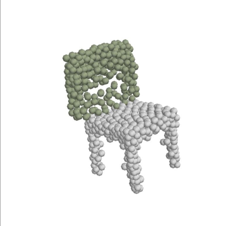
Our main contributions are summarised as follows.               points and shared ancestors. In addition, P OINT F LOW (Yang
1. We propose a framework for unsupervised parts-based             et al. 2019) learns a distribution of points based on a dis-
   point cloud generation.                                         tribution of shapes by combining VAE S and Normalizing
                                                                   Flows (Rezende and Mohamed 2015), from which a point
2. We achieve reliable disentanglement of the latents by
                                                                   set with variable number of points may be sampled. How-
   modeling points, primitives, and pose for each part.
                                                                   ever, all of the above works generate the point cloud as
3. We demonstrate controllable parts editing via disentan-         a whole or by a tree structure without disentanglement,
   gled point cloud latents for different parts.                   thereby limiting their application power in parts editing.
We provide extensive experimental results on S HAPE N ET           Although the work by Chen et al. (2019) focusing on re-
which quantitatively demonstrates the superior performance         construction could easily be adapted to unsupervised parts-
of our method as a generator of point clouds.                      based generation task, it does not infer precise pose infor-
                                                                   mation which is crucial in editing.
                      Related work                                    A few recent works (Nash and Williams 2017; Mo et al.
Disentangled Latent Representation in VAE. To promote              2019, 2020; Schor et al. 2019; Dubrovina et al. 2019) pro-
disentanglement beyond that of the vanilla VAE (Kingma             pose (or could be adapted) to generate point clouds given
and Welling 2014), Higgins et al. (2016) introduced an ad-         ground-truth point cloud parts segmentation. However, the
ditional KL divergence penalty above that of the usual evi-        requirement of well-aligned parts semantic labels hinders
dence lower bound (ELBO). Learning of disentangled latent          their real world applications. MRGAN (Gal et al. 2020)
representations is further investigated by Kim et. al (2018),      firstly attempts to address the parts-aware point cloud gen-
and Chen et al. (2018). To handle minibatches while ac-            eration by discovering parts of convex shape in an unsuper-
counting for the correlation of latents, Kim et. al (2018) pro-    vised fashion. While effective, the decomposed parts may
posed a neural-discriminator based estimation while Chen           lack semantic meaning. Following this line of work, our E D -
et al. (2018) introduced a minibatch-weighted approxima-           IT VAE approaches parts-aware generation without semantic
tion. Further, Kim et al. (2019c) split latent factors into rel-   label requirements. In addition, the proposed model learns a
evant and nuisance factors, treated each in a different man-       disentangled latent representation, so that the style and pose
ner within a hierarchical Bayesian model (2019b). Locatello        of parts can be edited independently.
et al. (2019a) showed that disentanglement may encourage
fairness with unobserved variables, and proved the impos-                                Preliminaries
sibility of learning disentangled representations without in-      To disentangle semantically relevant parts of a 3D point
ductive biases (2019b) in an unsupervised manner, while            cloud, we decompose it into latent parts which are modeled
showing that mild supervision may be sufficient (2020).            both as 3D point clouds and 3D shape primitives.
    To learn a reliable disentangled latent representation, the    A point cloud in RN ×3 is a set of N points sampled from
present work introduces a useful inductive bias (Locatello         the surface of 3D shape in Euclidean coordinates.
et al. 2019b) by jointly modeling points, primitives and           Primitives are simple shapes used to assemble parts of more
pose for 3D shapes. Inspired by the relevance and nuisance         complex shape. We employ the superquadric parameterisa-
factor separation (Kim et al. 2019b,c), this work observes         tion for the primitives, which is a flexible model that in-
and balances the conflict between disentanglement of rep-          cludes cubes, spheres and ellipsoids as special cases. In line
resentation and quality of generation, by separately model-        with Paschalidou, Ulusoy, and Geiger (2019), we formally
ing global correlations of the relative pose of the different      define our superquadric as the two dimensional manifold pa-
parts of a shape, disentangled from their style. Finally, we       rameterised by η and ω, with surface point
fill the gap of learning disentangled latent representations of                  "
                                                                                   αx cos1 η cos2 ω
                                                                                                      #
3D point cloud in an unsupervised manner, thereby contrast-                                             −π/2 ≤ η ≤ π/2
                                                                      r(η, ω) = αy cos1 η sin2 ω                        , (1)
ing with much recent disentangled representation learning                                    1          −π ≤ ω ≤ π
                                                                                       αz sin η
works focusing on 2D or supervised cases (Kalatzis et al.
2020; Nielsen et al. 2020; Sohn, Lee, and Yan 2015).               where α = (αx , αy , αz )> and  = (1 , 2 )> are the size and
Neural 3D Point Cloud Generation. While 2D image gen-              shape parameters, respectively. We include additional defor-
eration has been widely investigated using GAN S (Isola            mation parameters based on Barr (1987) in supplementary.
et al. 2017; Zhu et al. 2017) and VAE S (Kingma and Welling        Pose transformations are employed to map both the su-
2014; Higgins et al. 2016; Kim et al. 2019b; Sohn, Lee, and        perquadric and point cloud representations of the parts from
Yan 2015), neural 3D point cloud generation has only been          a canonical pose to the actual pose in which they appear in
explored in recent years. Achlioptas et al. (2018) first pro-      the complete point cloud. We parameterise this transforma-
posed the r-GAN to generate 3D point clouds, with fully            tion as x 7→ T (x) = R(q)x + t, which is parameterised by
connected layers as the generator. In order to learn local-        a translation t ∈ R3 and a rotation defined by the quaternion
ized features, Valsesia et al. (2018) and Shu et al. (2019) in-    q ∈ R4 . We refer to T as the pose for a given part.
troduced a generator based on Graph Convolutions. Specif-          Variational Auto-Encoders (VAE) (Kingma and Welling
ically, Shu et al. (2019) proposed a tree-based structure          2014) are an approximate Bayesian inference scheme that
with ancestors yielding a neighbor term and direct par-            introduces an approximate posterior Qφ (z|X) of the latent
ents yielding a loop term, named the T REE GAN. This de-           representation conditional on the point cloud X. The varia-
sign links the geometric relationships between generated           tional parameters φ are obtained by optimising a bound on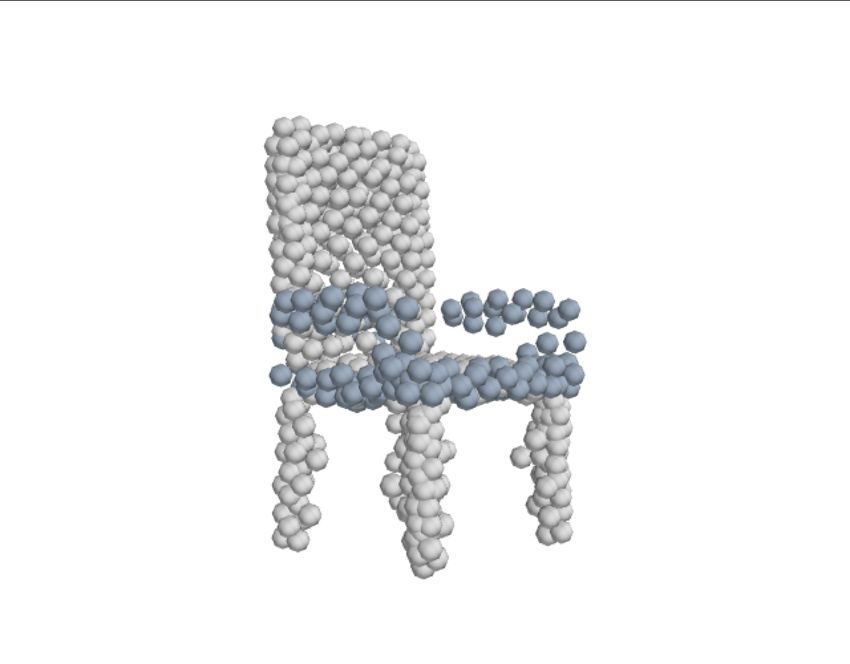
(m)
g T , gP
(m) P✓ (⇣|z) P✓ (X|⇣)
Mapping
Linear FC
gY
(m)
Ŷ1
Y1 Combined Point Cloud Y
(1) (1)
zY gY
T1
(1) (1)
zT gT
P̂1
P1 Assemble
(1) (1)
zP gP
Y2
Part Point Cloud
Ŷ2
Encoder Mapping zY
(2) (2)
gY
⌃ µ Sample T2
Q (z|X) z A zT
(2) (2)
gT
P2
P̂2
(2) (2)
Global Latent zP gP L
Y3
(3)
Ŷ3
(3) gY
zY
T3
(3) (3)
zT gT
P3
(3) (3)
P̂3 Assemble
zP gP
Input Point Cloud Disentangled Latent ⇣ Part Primitive Combined Primitives
X zl P
Figure 2: An overview of the E DIT VAE architecture. During training, the posterior is inferred by the encoder Qφ given the input
point cloud X, from which a global latent z is sampled. The global latent is linearly mapped by A to the disentangled latent
zl . The disentangled latent maps to parts (denoted by colors), which are further split into point Ŷm , pose Tm , and primitive P̂m
(i)
representations, via the deterministic mappings g? . Each point Ŷm and primitive P̂m is transformed to the global coordinate
system by the shared pose Tm . The transformed part points Ym and primitives Pm are then assembled to the complete decoded
point cloud Y and primitive P models, respectively. Jointly training with a single loss L (far right) parsimoniously models
key dependencies between point, primitive, and pose models. For generation, z is sampled from the standard Gaussian and fed
forward to generate point cloud Y .
the (marginal) data likelihood Pθ (X) known as the ELBO, 3. Representing the components of the above decomposi-
tion in a latent space which allows style and pose to be
log Pθ (X) ≥ EQφ (z|X) [log Pθ (X|z)]
manipulated independently of one another, while gener-
− DKL (Qφ (z|X))kP (z)) . (2) ating concrete and complete point clouds.
The first term is known as the reconstruction error, and the We address this problem in an end-to-end manner with a
second as the variational regulariser. We follow the usual unified probabilistic model. To accomplish this we depart
approach of letting the posterior Qφ (z|X) be multivariate slightly from the well known VAE structure, which directly
normal, so that we can employ the usual Monte Carlo ap- reconstructs the input by the decoder.
proximation with the reparameterisation trick (Kingma and For any given input point cloud X we generate a sepa-
Welling 2014) to approximate the reconstruction error. By rate point cloud Ŷm for each part m of the input point cloud
additionally letting the prior P (z) be multivariate normal, (such as the base of a chair), along with a super-quadric pro-
we obtain a closed form expression for the regulariser. totype P̂m of that part. This addresses point 1 above. To ad-
dress point 2, we model P̂m and Ŷm in a standardised refer-
Methodology ence pose via the affine transformation Tm , and denote by
We motivate our design in next subsection, and then intro-
duce our variational inference scheme, explain how we ob- Pm = Tm (P̂m ) and Ym = Tm (Ŷm ) (3)
tain disentanglement of part latents, give details of the loss
the point cloud and primitive part representations in the orig-
functions we use, and conclude with architecture details.
inal pose. This allows a part’s style to be edited while main-
Overview of the Design taining global coherance. Finally, while we model a single
global latent z, our decoder generates each part via separate
We divide the challenge of parts-based point cloud genera- network branches (see Figure 2), thereby facilitating various
tion and editing into the following essential challenges: editing operations and satisfying point 3 above.
1. Decomposing multiple (unlabeled) point clouds into se-
mantically meaningful parts. Variational Inference
2. Disentangling each part into both style (such as the shape Our approximate inference scheme is based on that of the
of the chair leg) and the relative pose (the orientation in VAE (Kingma and Welling 2014; Rezende, Mohamed, and
relation to the other parts of the chair). Wierstra 2014), but similarly to Kim et al. (2019a) relaxes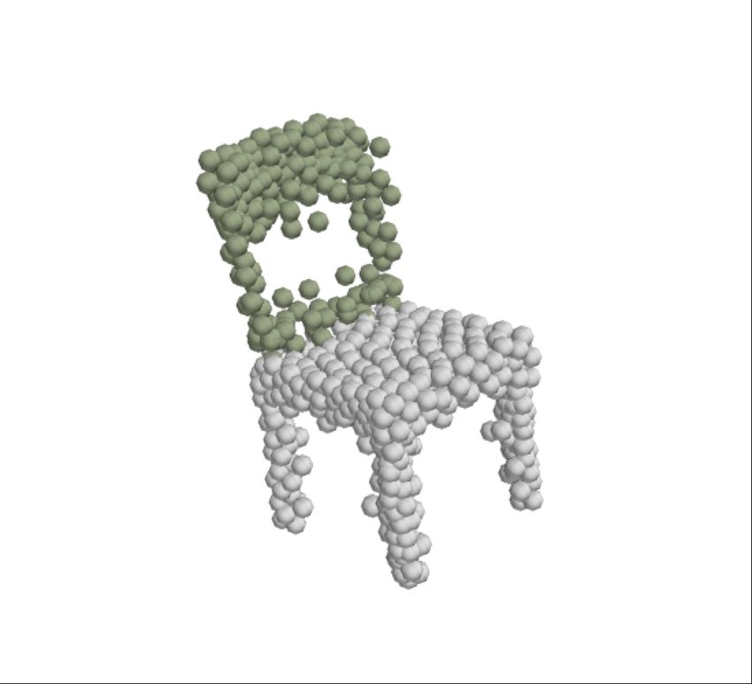
the assumption that the encoder and decoder map from and         and let the corresponding parts themselves be defined as
to the same (data) space. The following analysis is straight-                                   (m)   (m)
                                                                                      Ŷm = gY (zY ),                       (13)
forward, yet noteworthy in that it side-steps the inconve-
                                                                                                        (m)
nience of applying variational regularization to ζ.              and similarly for P̂m and Tm . Here,  gY     non-linearly trans-
   Denote by ζm = {Ŷm , P̂m , Tm } the m-th latent part rep-    forms from the latent space to the part representation.
                      SM                                            This achieves several goals. First, we inherit from the
resentation, by ζ = m=1 ζm the union of all such parts,
and by z a global latent which abstractly represents a shape.    VAE a meaningful latent structure on z. Second, by linearly
                                                                                                               (i)  (i)       (i)
We let Qφ (z, ζ|X) represent the approximate posterior with      mapping from z to the local part latents zY , zT and zP ,
parameters φ, and for simplicity we neglect to notate the de-    we ensure that linear operations (e.g. convex combination)
pendence of Qφ on θ. Our training objective is the usual         on the global latent precisely match linear operations on the
marginal likelihood of the data X given the parameters θ,        local latent space, which therefore captures a meaningfully
                         Z                                       local latent structure. Finally, partitioning zl yields a repre-
              Pθ (X) = Pθ (X, z, ζ) dz dζ.                (4)    sentation that disentangles parts by construction, while de-
                                                                 pendencies between parts are captured by A. Experiments
Taking logs and applying Jensen’s inequality we have             show we obtain meaningful disentangled parts latents.
                  Z
 log Pθ (X) = log Pθ (X, z, ζ) dz dζ                  (5)        Loss Functions
                                                                 Completing the model of the previous sub-section requires
                     Qφ (z, ζ|X)
                  Z
            = log                 Pθ (X, z, ζ) dz dζ (6)         to specify the log likelihood log Pθ (X|ζ), which we decom-
                     Qφ (z, ζ|X)                                 pose in the usual way as the negative of a sum of loss func-
              Z
                                  Pθ (X, z, ζ)                   tions involving either or both of the point Ym and super-
            ≥ Qφ (z, ζ|X) log                  dz dζ. (7)        quadric Pm , representations—combined with the standard-
                                  Qφ (z, ζ|X)                    isation transformation T which connects these representa-
We assume a chain-structured factorisation in our posterior,     tions to the global point cloud, X. Note that from a Bayesian
                                                                 modelling perspective, there is no need to separate the loss
             Pθ (z, ζ|X) = Pθ (ζ|z)Pθ (z|X).              (8)
                                                                 into terms which decouple P and Y ; indeed, the flexibility
Under this factorisation we obtain a tractable variational in-   to couple these representations within the loss is a source of
ference scheme by assuming that conditional on z, the ap-        useful inductive bias in our model.
proximate posterior matches the true one, i.e.                      While our loss does not correspond to a normalised condi-
            Qφ (z, ζ|X) ≡ Pθ (ζ|z) Qφ (z|X).              (9)    tional Pθ (X|ζ), working with un-normalised losses is both
                                                                 common (Sun et al. 2019; Paschalidou, Ulusoy, and Geiger
Putting (23) into (21) and cancelling Pθ (ζ|z) in the log in     2019), and highly convenient since we may engineer a prac-
(21),                                                            tically effective loss function by combining various carefully
    log Pθ (X) ≥ EQφ (z|X) [log Pθ (X|ζ)]                        designed losses from previous works.
                                                                 Point Cloud Parts Loss. We include a loss term for each
                          − DKL (Qφ (z|X))kPθ (z)) ,     (10)    part point cloud Ŷm based on the Chamfer distance
where ζ = NNθ (z). In a nutshell, this shows that we                 Lc (X, Y ) =                                          (14)
need only learn an approximate posterior Qφ (z|X) via a                1 X                           1   X
similar ELBO as (2), to obtain an approximate posterior                          min kx − yk22 +             min kx − yk22 .
                                                                     2|X|        y∈Y               2|Y |    x∈X
on ζ. We achieve this via a simple deterministic mapping                  x∈X                           y∈Y
which, like Nielsen et al. (2020), we may notate as the limit    We sum over parts to obtain a total loss of
Pθ (ζ|z) = Qφ (ζ|z) → δ(ζ−NNθ (z)), where δ is the Dirac                                 M
distribution and NNθ denotes a neural network. Crucially,
                                                                                        X
                                                                                LY =         Lc (X̂m , Ŷm ),               (15)
while the posterior in ζ is non-Gaussian, it doesn’t appear in                            m=1
the variational regulariser which is therefore tractable.        where Xm is the subset of X whose nearest superquadric is
Disentangling the Latent Representation                          Pm , and X̂m = T −1 (Xm ) is in canonical pose.
                                                                 Superquadric Losses. The remaining terms in our loss re-
E DIT VAE disentangles the global latent z into a local (to                                                 SM
                   (i)                                           late to the part Pm and combined P = m=1 Pm prim-
part ζm ) latent zl , and further to latents for specific com-   itives, and would match Paschalidou, Ulusoy, and Geiger
ponent of that part (namely Ym , Pm or Tm ). We achieve          (2019) but for the addition of a regulariser which discour-
this key feature by linearly transforming and partitioning the   ages overlapping superquadrics, i.e.1
global latent, i.e. we define
                                                                     Lo (P )                                            (16)
              (1)     (2)           (M ) >                                   M
           (zl , zl , · · · , zl       ) = zl = Az,      (11)            1 X        1        X
                                                                     =                              max (1 − Hm (s), 0) ,
where A is a matrix of weights (representing a linear neural             M m=1 |S| − |Sm |
                                                                                             s∈S\Sm
network layer). We further partition the part latents as
                                                                    1
                    (m)       (m)     (m)    (m)                      Lo (P ) matches the implementation of Paschalidou, Ulusoy,
               zl         = (zY , zT , zP )> ,           (12)    and Geiger (2019) provided by the authors.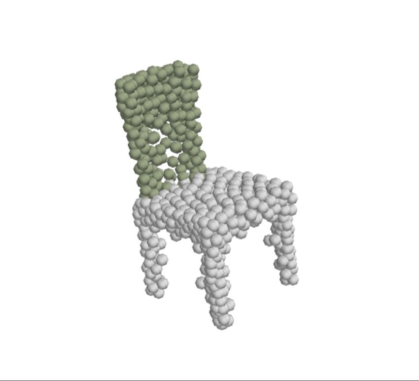
Table 1: Generative performance. ↑ means the higher the better, ↓ means the lower the better. The score is highlighted in bold
if it is the best one compared with state-of-the-art. Here M is the number of minimum parts we expect to separate in training.
For network with ? we use the result reported in (Valsesia, Fracastoro, and Magli 2018; Shu, Park, and Kwon 2019)

   Class                       Model                       JSD ↓   MMD-CD ↓          MMD-EMD ↓           COV-CD ↑       COV-EMD ↑
                                          ?
                       r-GAN (dense)                       0.238     0.0029               0.136               33               13
                        r-GAN (conv)?                      0.517     0.0030               0.223               23                4
                      Valsesia (no up.)?                   0.119     0.0033               0.104               26               20
   Chair                 Valsesia (up.)?                   0.100     0.0029               0.097               30               26
             T REE GAN (Shu, Park, and Kwon 2019)          0.119     0.0016               0.101               58               30
                    MRGAN (Gal et al. 2020)                0.246     0.0021               0.166               67               23
                      E DIT VAE (M=7)                      0.063     0.0014               0.082               46               32
                      E DIT VAE (M=3)                      0.031     0.0017               0.101               45               39
                       r-GAN(dense)?                       0.182     0.0009               0.094               31                9
                        r-GAN(conv)?                       0.350     0.0008               0.101               26                7
                      Valsesia (no up.)?                   0.164     0.0010               0.102               24               13
 Airplane               Valsesia (up.)?                    0.083     0.0008               0.071               31               14
             T REE GAN (Shu, Park, and Kwon 2019)          0.097     0.0004               0.068               61               20
                    MRGAN (Gal et al. 2020)                0.243     0.0006               0.114               75               21
                      E DIT VAE (M=6)                      0.043     0.0004               0.024               39               30
                      E DIT VAE (M=3)                      0.044     0.0005               0.067               23               17
             T REE GAN (Shu, Park, and Kwon 2019)          0.077     0.0018               0.082               71               48
   Table            MRGAN (Gal et al. 2020)                0.287     0.0020               0.155               78               31
                      E DIT VAE (M=5)                      0.081     0.0016               0.071               42               27
                      E DIT VAE (M=3)                      0.042     0.0017               0.130               39               30

where | · | denotes cardinality, Sm is a point cloud sampled       Baselines. We compare with four existing models of r-
                SM
from Pm , S = m=1 Sm , and Hm (·) is the smoothed indi-            GAN (Achlioptas et al. 2018), Valsesia (Valsesia, Fracas-
cator function for Pm defined in Solina and Bajcsy (1990).         toro, and Magli 2018), T REE GAN (Shu, Park, and Kwon
                                                                   2019) and MRGAN (Gal et al. 2020). r-GAN and Valsesia
Architecture Details                                               generate point clouds as a single whole without parts infer-
                                                                   ence or generation based on a tree structure as in T REE -
E DIT VAE framework is shown in Figure 2. The posterior            GAN. Similar to our approach, MRGAN performs unsu-
Qφ (z|X) is based on the P OINT N ET architecture (Qi et al.       pervised parts-aware generation, but with “parts” that lack a
2017), with the same structure as Achlioptas et al. (2018).        familiar semantic meaning and without disentangling pose.
For Pθ (ζ|z), we apply the linear transform and partitioning       Implementation details.2 The input point cloud consists of
of (11) for disentangled part representations followed by fur-     a set of 2048 points, which matches the above baselines. Our
ther shape and pose disentanglement. We use the generator          prior on the global latent representation z ∈ R256 is the
of T REE GAN (Shu, Park, and Kwon 2019) as the decoder,                                                             (m)
             (i)                                                   usual standard Gaussian distribution. We chose zY ∈ R32 ,
modelling gY , to generate the point cloud for each part. The             (m)    (m)
super-quadric decoder modules match Paschalidou, Ulusoy,           and zT , zP        ∈ R8 for the local latents of (12). We
and Geiger (2019) for primitive generation Pm , as do those        trained E DIT VAE using the A DAM optimizer (Kingma and
for the Tm . Weights are not shared among branches.                Ba 2015) with a learning rate of 0.0001 for 1000 epochs and
                                                                   a batch size of 30. To fine-tune our model we adopted the
                                                                   β-VAE framework (Higgins et al. 2016).
                      Experiments
Evaluation metrics. We evaluate our E DIT VAE on the               Results
ShapeNet (Chang et al. 2015) with the same data split              Generation. E DIT VAE generates point clouds by simply
as Shu, Park, and Kwon (2019) and report results on                sampling from a standard Gaussian prior for z, mapping by
the three dominant categories of chair, airplane, and ta-          A and and the subsequent part branches of Figure 2, be-
ble. We adopt the evaluation metrics of Achlioptas et al.          fore merging to form the complete point cloud. We show
(2018), including Jensen-Shannon Divergence (JSD), Mini-           quantitative and qualitative results in Table 1 and Figure 3,
mum Matching Distance (MMD), and Coverage (COV). As                respectively. As shown in Table 1, the proposed E DIT VAE
MMD and COV may be computed with either Chamfer Dis-               achieves competitive results (see e.g. the M = 7 results for
tance (CD) or Earth-Mover Distance (EMD), we obtain five           the chair category) compared with the states of the art. The
different evaluation metrics, i.e. JSD, MMD-CD, MMD-
                                                                      2
EMD, COV-CD, and COV-EMD.                                                 Code will be provided on publication of the paper.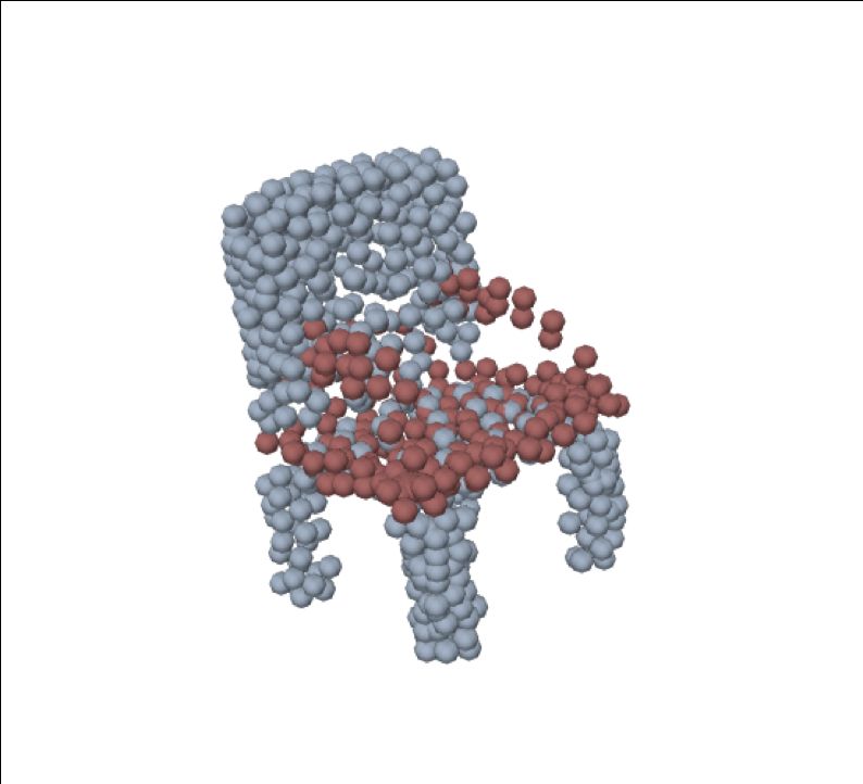
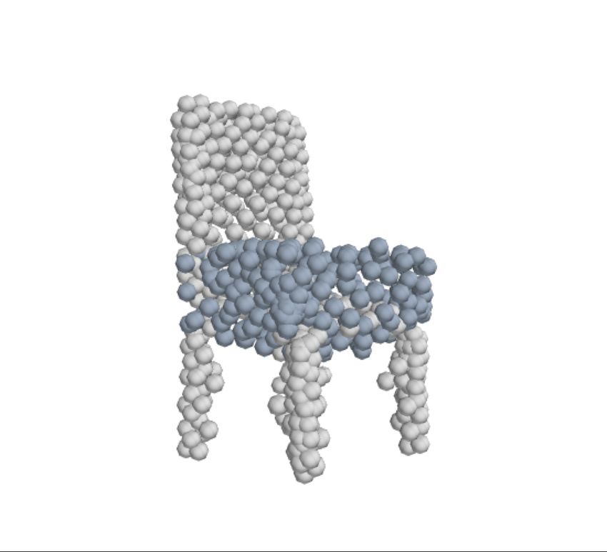
Figure 3: Parts-based generated point clouds from the airplane, table and chair categories, coloured by part. Bottom row:
examples generated by T REE GAN (Shu, Park, and Kwon 2019). The top three rows are E DIT VAE—the top row with M = 3,
and the second and third rows with the number of parts M reported in Table 1.

parts number M is manually selected to achieve a meaning-
ful semantic segmentation, e.g. a chair may be roughly de-
composed into back, base, and legs for M = 3. Furthermore,
while Shu, Park, and Kwon (2019) generates point clouds
according to a tree structure—and could thereby potentially
generate points with consistent part semantics—it does not
allow the semantics-aware shape editing due to lacking of
disentangled parts representations. To the best of our knowl-
edge, MRGAN (Gal et al. 2020) is the only other method
achieving parts-disentangled shape representation and gen-
eration in an unsupervised manner. The results in Table 1
show that our method outperforms MRGAN in both the JSD
and MMD metrics. Morover, E DIT VAE achieves highly se-
mantically meaningful parts generation as shown in Fig-
ure 3 and the experiment as discussed below, which further
achieves parts-aware point cloud editing.                         Figure 4: Parts mixing in the chair category with M = 3.
Parts Editing. E DIT VAE disentangles the point clouds into       Far left: ground truth point clouds, top: reference point
latents for each part, and then in turn into the point cloud,     cloud. Remaining: from left to right, back, base, and legs
pose, and primitive for each part. This design choice allows      for ground truth points are mixed by corresponding parts in
editing some parts with other parts fixed, yielding control-      the reference one via mixing their disentangled latents.
lable parts editing and generation. We demonstrate this via
both parts mixing and parts (re-)sampling.
Parts Mixing. It is defined by exchanging some parts be-          Parts Sampling. This involves resampling some parts in a
tween generated reference and ground-truth point clouds           generated point cloud. For resampled parts, we fix the pose
while keeping others fixed. We achieve mixing by transfer-        but resample the point cloud parts latent. The fixed pose is
ring corresponding parts latents from reference to ground-        essential to maintain generated part point clouds with a con-
truth, and further transforming it by the generator and pose      sistent location that matches the other fixed parts to achieve
of the parts in the ground-truth. The corresponding part in       controllable generation. Qualitative results for parts sam-
the ground-truth point cloud may therefore be changed to          pling are in Figure 5. Variations in the part styles demon-
the style of the reference one. For example, the results in the   strated the controllable point cloud generation.
first row of Figure 4 show that the ground-truth shape of a       Semantic Meaningfulness. We first define a vanilla mea-
sofa with solid armed base may be changed into a larger hol-      surement by comparing the distance between the ground
low armed one based on its reference shape with consistent        truth semantic label and the unsupervisedly generated one.
style. Namely, the size and pose of mixed parts follow that       The distance is defined as the mean of smallest Chamfer dis-
of the ground-truth, but keep the style from the reference.       tance for each unsupervised part with respect to all ground
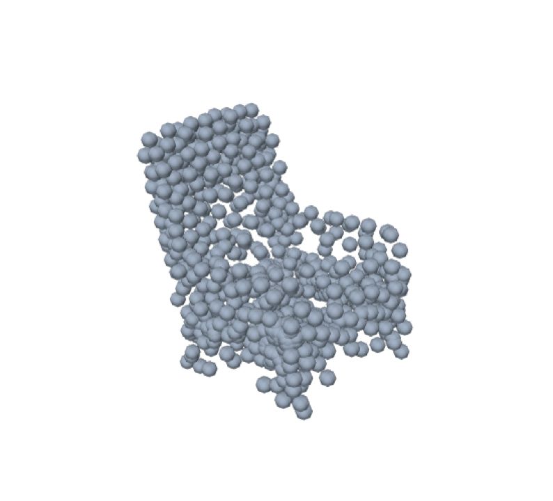
Table 2: Semantic meaningfulness measurements. M = ∗ represents E DIT VAE inTable 1. The lower MCD the better.

                                     Chair                             Airplane                               Table
           Model
                      T REE GAN        M=3         M=7        T REE GAN    M=3         M=6       T REE GAN      M=3        M=5
           MCD↓          0.0164       0.0028      0.0121           0.0043   0.0016    0.0018       0.0266       0.0121    0.0214

Table 3: Generative performance for the entire shape and its
parts, for the chair category. Semantic labels are obtained by
primitive segmentation in our framework.

                                     MMD-CD↓
        Model
                     as whole        base back               leg
   E DIT VAE           0.0017       0.0016    0.0014     0.0024
   BASELINE            0.0025       0.0017    0.0015     0.0024

Table 4: Generative performance comparsion for E DIT VAE
and two baselines in chair category.
                                                                            Figure 5: Parts sampling. Far left: the reference point clouds.
                                                                            Colored parts in the three right columns are sampled from
           Model            JSD↓      MMD-CD↓          COV-CD↑              latent space—from top to bottom, we sampled the airplane
     Baseline-G             0.062        0.0019              42             stabilizer, chair base, and chair back.
     Baseline-S             0.163        0.0030              10
  E DIT VAE (M=3)           0.031        0.0017              45
  E DIT VAE (M=7)           0.063        0.0014              46             a supervised parts-aware generation approach (Schor et al.
                                                                            2019). Baseline-G is created by training the the point cloud
                                                                            branch in Figure 2 with the ground-truth parts segmenta-
                                                                            tion. The comparison is performed on the chair category in
truth parts (MCD in Table 2). As MRGAN (Gal et al. 2020)
                                                                            S HAPE N ET (Chang et al. 2015), and reported in Table 4.
lacks accompanying code, we mainly compare the semantic
                                                                               E DIT VAE is robust to semantic segmentation as its gen-
meaningfulness with respect to T REE GAN in Table 2. E D -
                                                                            eration is close to Baseline-G. Further, the performance of
IT VAE outperforms when we define the ground truth seg-
                                                                            M = 3 is closer to Baseline-G compared with M = 7,
mentation as the most meaningful.
                                                                            in line with our observation (see Figure 3) that this case
                                                                            achieves a similar segmentation to the ground-truth. Fur-
Ablation Studies                                                            ther, E DIT VAE outperforms Baseline-S by overcoming the
Generation / Editing Trade-Off. We aim to evaluate the                      style-mismatch issue and is robust to noise introduced by
influence of the linear mapping A for disentangled repre-                   mapping parts to a canonical system with learned poses.
sentation learning (see Figure 2). To this end, we introduce
a BASELINE framework by simply removing this A. Results                                            Conclusions
are shown in Table 3. Specifically, we compare our gener-                   We introduced E DIT VAE, which generates parts-based
ation with the BASELINE results at the whole point cloud                    point clouds in an unsupervised manner. The proposed
level and at the parts level, such as the base, leg, and back,              framework learns a disentangled latent representation with a
for the chair category. While BASELINE achieves disentan-                   natural inductive bias that we introduce by jointly modeling
gled parts-aware representation learning and comparable re-                 latent part- and pose-models, thereby making parts control-
sults for parts sampling to E DIT VAE3 , the manner in which                lable. Through various experiments, we demonstrated that
BASELINE generates points as a whole via sampling from                      E DIT VAE balances parts-based generation and editing in
a standard Gaussian yields inferior performance due to the                  a useful way, while performing strongly on standard point-
mismatched style across parts. Thus, the mapping A man-                     cloud generation metrics.
ages to decouple the undesirable generation / editing trade-
off caused by disentanglement. Detailed analysis and visu-
alizations are in the supplementary materials.
Stage-wise Baselines. We compared E DIT VAE with two
stage-wise baselines defined as Baseline-S and Baseline-G.
In particular, Baseline-S is built by first generating parts
labels via the state-of-the-art unsupervised segmentation
method (Paschalidou, Ulusoy, and Geiger 2019) followed by
   3
       We evaluate each part generation result separately.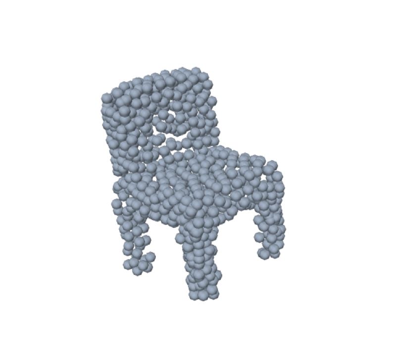
Generation / Editing Trade-off Analysis &
                    Results
We aim to evaluate the influence of the linear mapping A
for disentangled representation learning (see Figure 2 in the
main paper). To this end, we introduce a BASELINE frame-
work by simply removing this A. Results are shown in the
main paper Table 3. Specifically, we compare our genera-
tion with the BASELINE results at the whole point cloud
level and at the parts level, such as the base, leg, and back,
for the chair category. While BASELINE achieves disentan-
gled parts-aware representation learning and comparable re-
sults for parts sampling to E DIT VAE the manner in which
BASELINE generates points as a whole via sampling from
a standard Gaussian yields inferior performance due to the
mismatched style across parts.
   We observe that well-disentangled latents benefit control-
lable editing, as we may unilaterally alter the style of one
part, without affecting that of the other parts. This is mainly
due to our particular disentangled representation which dis-
courages certain dependencies among latents. By contrast,
parts-based generation requires strong correlation within la-
tent factors to generate style-matched point clouds. Hence,       Figure 6: Visualization of point clouds generated by E DIT-
this disentanglement is fundamentally opposing to the parts-      VAE (below lines) and BASELINE (above lines). Colors de-
based point cloud generation as a whole due to the lack of        note the different parts.
global correlation across parts.
   This observation can be further explained by the concept
of relevant and nuisance latents separation in (Kim et al.        dle left) and fighter’s wings (middle right) being assembled
2019c) which addresses the balance between reconstruction         with civil airliners. Moreover, as sampled pose latents are
and generation. Specifically, relevant latents depend on the      mismatched with sampled point latents, the stabilizers are
input and vice versa, which indicates that the global “style”     added at the wrong position (left most).
information is stored in the relevant latent. Completely dis-        In summary, the ‘style’ of parts is mismatched in point
entangled latents can achieve perfect reconstruction, as the      clouds generated by BASELINE, mainly because the disen-
known inputs can lead to fully observed relevant and nui-         tangled latents do not keep the global correlations within
sance latents. However, relevant latents are randomly sam-        parts. By contrast, our model can generate point clouds in a
pled in generation due to the lack of input as observation.       consistent style due to our global context-aware latents dis-
As a result, disentangled latents with different ”style” infor-   entanglement which is achieved by the linear mapping A in
mation lead to a style mismatch across the generated part         our framework.
point clouds. We thus introduce a linear mapping A to en-
code the ”relevant” latents consistently across disentangled                  Additional Mixing Examples
part latents, to achieve parts-aware generation with a consis-    In the main paper we showed parts mixing results for the
tent style.                                                       chair category in S HAPE N ET (Chang et al. 2015) with num-
   We provide more quantitative results in Table 5. Similar       ber of primitives M = 3. Here we will provide more parts
to the results reported in Table 1 of the main paper, we com-     mixing results on other categories.
pare the generative performance of E DIT VAE with a BASE -           In Figure 7, we mix parts in the airplane category with
LINE for which we removed the linear mapping A from our           number of primitives M = 6. Each ground truth point cloud
model. As shown in Table 5, the proposed E DIT VAE con-           (blue) is mixed with a reference point cloud (red) with re-
sistently outperforms the BASELINE for all three categories       spect to the stabilizer, the right wing, and the engine. In the
and for various numbers of primitives M . The quantitative        first column of Figure 7, the shapes of all stabilizers in the
results demonstrate that sampling from disentangled latents       ground truth point clouds are changed to that of the reference
without global context information leads to point clouds of       one but respecting their poses, which leads to a mixed point
low quality. More qualitative comparison results are pro-         cloud with consistent style. In addition, the ground truth
vided in Figure 6, which shows that the style and pose are        airplanes without engines are also ‘assembled’ with refer-
mismatched in general among parts for point clouds gen-           ence’s engine by the mixing operation. It is worth noting
erated by BASELINE. For example, back parts in the chair          that the style of remaining parts has not been changed thanks
category either intersect the base (left most), or are detached   to our learned disentangled representation. Similar observa-
from it (third column). In addition, the back sizes are also      tions can be found in Figure 8. We additionally show our
not matched to the bases (all four examples). For airplanes       mixing results on the table category in Figure 9. As demon-
generated by BASELINE, we observe glider’s wings (mid-            strated in the figure, we can change the round base of the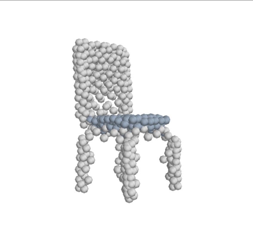
Table 5: More results in generation/editing trade-off

                                                                                          MMD-CD ↓
   Class     Primitive Number         Model
                                                  as whole        part A      part B     part C part D        part E     part F    part G
                                    E DIT VAE      0.0014         0.0012      0.0011     0.0015     0.0013    0.0025    0.0015    0.0013
                      7
                                    BASELINE       0.0029         0.0014      0.0012     0.0019     0.0014    0.0027    0.0016    0.0015
   Chair
                                    E DIT VAE      0.0017         0.0014      0.0016     0.0024        -         -         -         -
                      3
                                    BASELINE       0.0025         0.0016      0.0016     0.0024        -         -         -         -
                                    E DIT VAE      0.0004         0.0004      0.0005    0.00004     0.0006    0.0006    0.0005       -
                      6
                                    BASELINE       0.0007         0.0004      0.0005     0.0005     0.0006    0.0007    0.0005       -
 Airplane
                                    E DIT VAE      0.0005         0.0006      0.0005     0.0007        -         -         -         -
                      3
                                    BASELINE       0.0006         0.0006      0.0005     0.0008        -         -         -         -
                                    E DIT VAE      0.0016         0.0020      0.0011     0.0023     0.0015    0.0020       -         -
                      5
                                    BASELINE       0.0042         0.0024      0.0011     0.0030     0.0016    0.0022       -         -
   Table
                                    E DIT VAE      0.0017         0.0025      0.0012     0.0022        -         -         -         -
                      3
                                    BASELINE       0.0035         0.0034      0.0013     0.0025        -         -         -         -

                                                                           Figure 8: Parts mixing in the airplane category with M = 3.
                                                                           Far left: ground truth point clouds, top: the reference point
                                                                           cloud. Remaining: from left to right: the wings, stabilizer,
                                                                           and body for ground truth points are replaced by the corre-
Figure 7: Parts mixing in the airplane category with M = 6.                sponding parts in the reference one via mixing their disen-
Far left: ground truth point clouds, top: reference point                  tangled latents.
cloud. Remaining: from left to right: stabilizer, right wing,
and engine of the ground truth point clouds are replaced by
corresponding ones in the reference via mixing of their dis-
entangled latents.
                                                                           the Real NVP layer is linear, as it can be included in gener-
                                                                           ators/decoders. In order to have a simple and elegant model,
                                                                           we removed the Real NVP layer in the main paper.
table to a rectangular one from the reference point cloud in
a consistent style.                                                           Additional parts sampling results may be found in Fig-
                                                                           ures 10 and 11. We sampled chair legs and table right legs
           Additional Sampling Examples                                    in Figure 10. In particular, different styles (normal or sofa
                                                                           style), sizes (thick or slim), and pose (rotation) of legs are
As the parts distribution is unknown, we achieve parts sam-                sampled from our disentangled latents. Moreover, we pro-
pling by first sampling a global latent from a multivariate                vide more results for parts sampling of table bases and air-
normal distribution and then passing to the linear mapping                 plane wings in Figure 11.
A. Another option is passing the parts latent to a Real NVP
layer (Dinh, Sohl-Dickstein, and Bengio 2016) before feed-                    As shown in the figure, different shapes of table base
ing to the generators/decoders during training. By letting                 (round, rectangular and square), and styles of airplane wing
Real NVP learn to map the parts latent into a standard nor-                (glider’s and fighter’s wing) are sampled while the remain-
mal distribution, we may then generate novel parts by sam-                 ing parts are held fixed. We see that parts sampling allows
pling the parts latent directly. Both options are equivalent if            us to achieve controllable point clouds generation.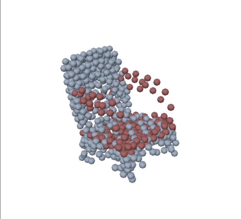
Figure 9: Parts mixing in the table category with M = 3. Far Figure 10: Parts sampling. Far left: the reference point
left: ground truth point clouds, top: reference point cloud. clouds. Colored parts in the three right columns are sampled
Remaining: from left to right: right legs, left legs, and base from the latent space —from top to bottom, we sampled the
for ground truth points are replaced by the corresponding chair legs and table legs.
parts in the reference one via mixing of the disentangled la-
tents.
Interpolation
Two generated point clouds are interpolated by first mix-
ing corresponding latents with different weights, and then
pass it to corresponding generators. The visualization re-
sults is shown in Figure 12. As we can see, the middle three
point clouds are deforming continuously from the leftmost
to rightmost. Thus, the learned latent space is continuous.
Semantic meaningfulness
Note that the Arxiv paper MRGAN (Gal et al. 2020) lacks Figure 11: Parts sampling. Far left: the reference point
accompanying code, we only compared semantic meaning- clouds. Colored parts in the three right columns are sampled
fulness with T REE GAN (Shu, Park, and Kwon 2019) quan- from the latent space —from top to bottom, we sampled the
titatively in the main paper. Here we show the qualitative table base and airplane wings.
comparison with MRGAN (Gal et al. 2020) via their main
Figure 3 and supplmentary Figure 1: For example, MR- ing deformation K is defined by:
GAN’s table bases are separated into three parts, some of k1
them even linked to a leg, while E DIT VAE separates base αz xz 0 0 "xx #
k2
and legs more clearly as per rows 2-3 in the main paper Fig- K(x) = 0 αz xz 0 xy , (17)
ure 3. 0 0 1 xz
where x = (xx , xy , xz )> is a point, and k = (k1 , k2 )> de-
Superquadrics visualization fines deformation parameters, and αz is the size parameter
in the z-axis. This linear taper deforms the primitive shape
See Figure 13 for an example for the generated su- in the x, y-axis by an amount which depends on the value of
perquadrics by passing sampled latents into pose and primi- the z-axis. As a result, tapering deformation will make prim-
tive branches in the main paper Figure 3. itives more conic, which helps to model unbalanced shapes
such as the head of the airplane.
Primitive Detail
Details on the Superquadric Losses
Deformation While the definition our superquadric loss functions fol-
lows Paschalidou, Ulusoy, and Geiger (2019), we include
As mentioned in Preliminaries of the main paper, we use a more details here for the sake of completeness.
tapering deformation (Barr 1987) to enhance the represen- The superquadric loss is defined as
tation power of the superquadrics. Following the code pro-
vided by Paschalidou, Ulusoy, and Geiger (2019), the taper- Ls (P , X) = LD (P , X) + Lr (P ), (18)First derivation By putting (22) and (23) into the lower
bound (21), we have
log Pθ (X) ≥ (24)
Pθ (ζ|z)Pθ (z|X)Pθ (X)
Z
Figure 12: Interpolation result. Leftmost to rightmost by Pθ (ζ|z) Qφ (z|X) log dz dζ.
Pθ (ζ|z) Qφ (z|X)
mixing latents with weights 0.2, 0.5, 0.8, respectively.
By cancelling Pθ (ζ|z) and taking the integral of ζ we get
Pθ (z|X)Pθ (X)
Z
log Pθ (X) ≥ Qφ (z|X) log dz. (25)
Qφ (z|X)
By applying Bayes’ rule, we have
Figure 13: Generated Superquadrics. Listed chair’s M = 3, Pθ (X|z)Pθ (z)
Z
table’s M = 5, airplane’s M = 6 as in Table 1 in main log Pθ (X) ≥ Qφ (z|X) log dz (26)
Qφ (z|X)
paper. Z
where LD is the distance term which encourages su- = Qφ (z|X) log Pθ (X|z) dz
perquadric P to fit the input point cloud X. Lr is a regu-
Qφ (z|X)
Z
larisation term which encourages desired behaviour; for ex- − Qφ (z|X) log dz. (27)
ample, we prefer primitives that do not overlap one another. Pθ (z)
The distance term measures the distance between points We see the key point, that the final term in (27) is tractable
sampled from primitive surface and input point cloud X. as it does not depend on ζ, that is DKL (Qφ (z|X))kPθ (z)).
Following the idea of the Chamfer distance, the distance Since our decoder has a simple deterministic relationship
term is decomposed by: which we denote by the limit
LD (P, X) = LP→X (P, X) + LX→P (X, P), (19) Qφ (ζ|z) → δ(ζ − NNθ (z)), (28)
where LP→X defines the distance from the primitive P to we can rewrite the reconstruction error term to emphasise
the input point cloud X, and LX→P defines the distance the dependence of X on ζ to get the ELBO
from the point cloud X to primitive P. Additional details
may be found in (Paschalidou, Ulusoy, and Geiger 2019). log Pθ (X) ≥ EQφ (z|X) [log Pθ (X|ζ)]
The regularisation term is defined as − DKL (Qφ (z|X))kPθ (z)) , (29)
Lr (P ) = ωo Lo (P ). (20) where ζ = NNθ (z).
As we manually select the number of parts, we only Second Derivation Using (22) and (23) in (21), we have:
use an overlapping regularizer to discourage the su- Pθ (X, z, ζ)
Z
perquadrics from overlapping one another; this term is log Pθ (X) ≥ Qφ (z, ζ|X) log dz dζ
Pθ (ζ|z) Qφ (z|X)
adapted from (Paschalidou, Ulusoy, and Geiger 2019).
Pθ (X|z, ζ)Pθ (z, ζ)
Z
In order to achieve the best performance, different ωo are = Qφ (z, ζ|X) log dz dζ
used for different categories during training. In particular we Qφ (z, ζ|X)
set: ωo = 1e − 6 for the chair category with number of = EQφ (z,ζ|X) [log Pθ (X|z, ζ)]
primitives M = 3; ω0 = 1e − 5 for the chair category with | {z }
L
M = 7, and the airplane category with M = 3 and M = 6 ;
ωo = 1e−10 for the table category with M = 3 and M = 5. Qφ (z, ζ|X)
− EQφ (z,ζ|X) log . (30)
Pθ (z, ζ)
Model details | {z
R
}
We give two alternative derivations of our training objective, The key point is revealed, that the regulariser term is
followed by some additional discussions, and details of our tractable because, by (23)
network architectures.
Qφ (z, ζ|X)
Detailed Derivations R = EQφ (z,ζ|X) log (31)
Pθ (z, ζ)
To make the supplementary material self contained, we first
Pθ (ζ|z)Qφ (z|X)
recall inequality (7) in the main paper, = EQφ (z,ζ|X) log (32)
Pθ (ζ|z)Pθ (z)
Pθ (X, z, ζ)
Z
log Pθ (X) ≥ Qφ (z, ζ|X) log dz dζ, (21) Qφ (z|X)
Qφ (z, ζ|X) = EQφ (z,ζ|X) log (33)
Pθ (z)
as well as equations (8) and (9) in the main paper,
Qφ (z|X)
= EQφ (z|X) log (34)
Pθ (z, ζ|X) = Pθ (ζ|z)Pθ (z|X), (22) Pθ (z)
Qφ (z, ζ|X) ≡ Pθ (ζ|z) Qφ (z|X). (23) = DKL (Qφ (z|X)kPθ (z)) . (35)Finally, since our decoder has a simple deterministic rela- factor for each layer are [32, 32, 16, 16, 3] and [1, 2, 4, 32],
tionship which we denote by the limit respectively. Hence, each point decoder outputs 256 points.
Pose and Primitive Decoders All pose and primitive de-
Qφ (ζ|z) → δ(ζ − NNθ (z)), (36) coders are one layer fully connected networks, follow-
we can rewrite the reconstruction error term to emphasise ing (Paschalidou, Ulusoy, and Geiger 2019). The dimension
the dependence of X on ζ, of the fully connected layers depends on the input latent size
(namely 8) and output parameter dimension. See the repos-
L = EQφ (z,ζ|X) [log Pθ (X|z, ζ)] (37) itory of (Paschalidou, Ulusoy, and Geiger 2019) for the de-
= EQφ (z|X) [log Pθ (X|ζ)] , (38) tailed implementation.
where in the final line ζ = NNθ (z). References
Achlioptas, P.; Diamanti, O.; Mitliagkas, I.; and Guibas, L.
Discussion 2018. Learning representations and generative models for
Because of the deterministic mapping between ζ and z, 3d point clouds. In International conference on machine
we have Pθ (ζ|z) = Qθ (ζ|z). This allows us to annotate learning, 40–49. PMLR.
Pθ (ζ|z) as in Figure 2 of the main paper. Barr, A. H. 1987. Global and local deformations of solid
In that same figure, we annotate with Pθ (X|ζ) the map- primitives. In Readings in Computer Vision, 661–670. Else-
ping (on the right hand side) from parts representations ζ vier.
to the output point cloud Y , despite X appearing on the
left hand side. This is consistent with standard expositions: Bongsoo Choy, C.; Stark, M.; Corbett-Davies, S.; and
for example, we may connect this with Appendix C.1 of the Savarese, S. 2015. Enriching object detection with 2d-3d
VAE paper (Kingma and Welling 2014) by noting that our Y registration and continuous viewpoint estimation. In Pro-
and P are together analogous to their Bernoulli parameters ceedings of the IEEE Conference on Computer Vision and
p. Pattern Recognition, 2512–2520.
Finally note that the posterior of, for example, the com- Chang, A. X.; Funkhouser, T.; Guibas, L.; Hanrahan, P.;
bined primitive P is not included in our variational infer- Huang, Q.; Li, Z.; Savarese, S.; Savva, M.; Song, S.; Su,
ence model, which is a byproduct obtained by assembling H.; Xiao, J.; Yi, L.; and Yu, F. 2015. ShapeNet: An
the part primitives from posterior samples of ζ. Information-Rich 3D Model Repository. Technical Report
arXiv:1512.03012 [cs.GR], Stanford University — Prince-
Architecture and Implementation Details ton University — Toyota Technological Institute at Chicago.
The model is implemented using PyTorch (Paszke et al. Chen, R. T. Q.; Li, X.; Grosse, R.; and Duvenaud, D. 2018.
2019) on the platform of Ubuntu 16.04, trained on one Isolating Sources of Disentanglement in Variational Autoen-
GeForce RTX 3090 and one GeForce RTX 2080 TI. 10 Gi- coders. Advances in Neural Information Processing Sys-
gabytes memory is allocated. tems.
The number of parts (parameter M ) for each category Chen, Z.; Yin, K.; Fisher, M.; Chaudhuri, S.; and Zhang,
is manually selected with domain specific knowledge. The H. 2019. BAE-NET: branched autoencoder for shape co-
choice reflects what one believes a good semantic segmen- segmentation. In Proceedings of the IEEE/CVF Interna-
tation should be, which is application dependent. As men- tional Conference on Computer Vision, 8490–8499.
tioned in the main paper, a chair may be roughly decom-
posed into back, base and legs for M = 3. In addition, a Dinh, L.; Sohl-Dickstein, J.; and Bengio, S. 2016. Density
chair could also be decomposed into back, base, armrest, estimation using real nvp. arXiv preprint arXiv:1605.08803.
and four legs for M = 7. For the airplane category, it could Dubrovina, A.; Xia, F.; Achlioptas, P.; Shalah, M.; Groscot,
separated into body, tail, and wings for M = 3; and also R.; and Guibas, L. J. 2019. Composite shape modeling via
into body, two wings, two engines, and tail for M = 6. Fi- latent space factorization. In Proceedings of the IEEE/CVF
nally, a table may be decomposed into base and four legs International Conference on Computer Vision, 8140–8149.
for M = 5; and also into base, left two legs, and right two Gal, R.; Bermano, A.; Zhang, H.; and Cohen-Or, D.
legs for M = 3. The general message here is clear: various 2020. MRGAN: Multi-Rooted 3D Shape Generation
decompositions are valid and useful. with Unsupervised Part Disentanglement. arXiv preprint
Encoder We use P OINT N ET (Qi et al. 2017) as the en- arXiv:2007.12944.
coder. Following the network structure from (Achlioptas
et al. 2018), the encoder has 64, 128, 128, 256 filters at each Higgins, I.; Matthey, L.; Pal, A.; Burgess, C.; Glorot, X.;
layer. Batch normalization and L EAKY R E LU are used be- Botvinick, M.; Mohamed, S.; and Lerchner, A. 2016. beta-
tween each layer. vae: Learning basic visual concepts with a constrained vari-
Point Decoder We use the generator of TreeGAN (Shu, ational framework.
Park, and Kwon 2019) as the point decoder. The architecture Isola, P.; Zhu, J.-Y.; Zhou, T.; and Efros, A. A. 2017. Image-
we used has 5 layers, with the root being the local part la- to-image translation with conditional adversarial networks.
tent vector, and the leaves being points in R3 . The loop term In Proceedings of the IEEE conference on computer vision
has K = 10 supports. The feature dimension and branching and pattern recognition, 1125–1134.Kalatzis, D.; Eklund, D.; Arvanitidis, G.; and Hauberg, S. Nielsen, D.; Jaini, P.; Hoogeboom, E.; Winther, O.; and
2020. Variational Autoencoders with Riemannian Brown- Welling, M. 2020. SurVAE Flows: Surjections to Bridge
ian Motion Priors. In Proceedings of the 37th International the Gap between VAEs and Flows. In Advances in Neu-
Conference on Machine Learning, ICML 2020, 13-18 July ral Information Processing Systems 33: Annual Conference
2020, Virtual Event, volume 119 of Proceedings of Machine on Neural Information Processing Systems 2020, NeurIPS
Learning Research, 5053–5066. PMLR. 2020, December 6-12, 2020, virtual.
Kim, H.; and Mnih, A. 2018. Disentangling by factorising. Paschalidou, D.; Ulusoy, A. O.; and Geiger, A. 2019. Su-
In International Conference on Machine Learning, 2649– perquadrics revisited: Learning 3d shape parsing beyond
2658. PMLR. cuboids. In Proceedings of the IEEE/CVF Conference on
Kim, J.; Oh, T.-H.; Lee, S.; Pan, F.; and Kweon, I. S. 2019a. Computer Vision and Pattern Recognition, 10344–10353.
Variational Prototyping-Encoder: One-Shot Learning with Paszke, A.; Gross, S.; Massa, F.; Lerer, A.; Bradbury, J.;
Prototypical Images. In Proceedings of the IEEE Conference Chanan, G.; Killeen, T.; Lin, Z.; Gimelshein, N.; Antiga, L.;
on Computer Vision and Pattern Recognition, 9462–9470. et al. 2019. Pytorch: An imperative style, high-performance
Kim, M.; Wang, Y.; Sahu, P.; and Pavlovic, V. 2019b. Bayes- deep learning library. Advances in neural information pro-
factor-vae: Hierarchical bayesian deep auto-encoder models cessing systems, 32: 8026–8037.
for factor disentanglement. In Proceedings of the IEEE/CVF Qi, C. R.; Su, H.; Mo, K.; and Guibas, L. J. 2017. Pointnet:
International Conference on Computer Vision, 2979–2987. Deep learning on point sets for 3d classification and segmen-
Kim, M.; Wang, Y.; Sahu, P.; and Pavlovic, V. 2019c. Rele- tation. In Proceedings of the IEEE conference on computer
vance factor vae: Learning and identifying disentangled fac- vision and pattern recognition, 652–660.
tors. arXiv preprint arXiv:1902.01568. Rezende, D.; and Mohamed, S. 2015. Variational inference
Kingma, D. P.; and Ba, J. 2015. Adam: A Method for with normalizing flows. In International Conference on Ma-
Stochastic Optimization. In 3rd International Conference chine Learning, 1530–1538. PMLR.
on Learning Representations, ICLR 2015, San Diego, CA, Rezende, D. J.; Mohamed, S.; and Wierstra, D. 2014.
USA, May 7-9, 2015, Conference Track Proceedings. Stochastic Backpropagation and Approximate Inference in
Kingma, D. P.; and Welling, M. 2014. Auto-Encoding Vari- Deep Generative Models. In Xing, E. P.; and Jebara, T.,
ational Bayes. In 2nd International Conference on Learning eds., Proceedings of the 31st International Conference on
Representations, ICLR 2014, Banff, AB, Canada, April 14- Machine Learning, volume 32 of Proceedings of Machine
16, 2014, Conference Track Proceedings. Learning Research, 1278–1286. Bejing, China: PMLR.
Locatello, F.; Abbati, G.; Rainforth, T.; Bauer, S.; Schor, N.; Katzir, O.; Zhang, H.; and Cohen-Or, D. 2019.
Schölkopf, B.; and Bachem, O. 2019a. On the Fairness of Componet: Learning to generate the unseen by part synthe-
Disentangled Representations. In Advances in Neural Infor- sis and composition. In Proceedings of the IEEE/CVF Inter-
mation Processing Systems 32: Annual Conference on Neu- national Conference on Computer Vision, 8759–8768.
ral Information Processing Systems 2019, NeurIPS 2019,
December 8-14, 2019, Vancouver, BC, Canada, 14584– Shu, D. W.; Park, S. W.; and Kwon, J. 2019. 3d point
14597. cloud generative adversarial network based on tree struc-
tured graph convolutions. In Proceedings of the IEEE/CVF
Locatello, F.; Bauer, S.; Lucic, M.; Raetsch, G.; Gelly, S.; International Conference on Computer Vision, 3859–3868.
Schölkopf, B.; and Bachem, O. 2019b. Challenging com-
mon assumptions in the unsupervised learning of disentan- Sohn, K.; Lee, H.; and Yan, X. 2015. Learning struc-
gled representations. In international conference on ma- tured output representation using deep conditional genera-
chine learning, 4114–4124. PMLR. tive models. Advances in neural information processing sys-
tems, 28: 3483–3491.
Locatello, F.; Tschannen, M.; Bauer, S.; Rätsch, G.;
Schölkopf, B.; and Bachem, O. 2020. Disentangling Fac- Solina, F.; and Bajcsy, R. 1990. Recovery of parametric
tors of Variations Using Few Labels. In 8th International models from range images: The case for superquadrics with
Conference on Learning Representations, ICLR 2020, Addis global deformations. IEEE transactions on pattern analysis
Ababa, Ethiopia, April 26-30, 2020. OpenReview.net. and machine intelligence, 12(2): 131–147.
Mo, K.; Guerrero, P.; Yi, L.; Su, H.; Wonka, P.; Mitra, N. J.; Sun, C.-Y.; Zou, Q.-F.; Tong, X.; and Liu, Y. 2019. Learning
and Guibas, L. J. 2019. StructureNet: hierarchical graph net- adaptive hierarchical cuboid abstractions of 3d shape collec-
works for 3D shape generation. ACM Trans. Graph., 38(6): tions. ACM Transactions on Graphics (TOG), 38(6): 1–13.
242:1–242:19. Valsesia, D.; Fracastoro, G.; and Magli, E. 2018. Learning
Mo, K.; Wang, H.; Yan, X.; and Guibas, L. 2020. PT2PC: localized generative models for 3d point clouds via graph
Learning to generate 3d point cloud shapes from part tree convolution. In International conference on learning repre-
conditions. In European Conference on Computer Vision, sentations.
683–701. Springer. Yang, G.; Huang, X.; Hao, Z.; Liu, M.-Y.; Belongie, S.; and
Nash, C.; and Williams, C. K. 2017. The shape variational Hariharan, B. 2019. Pointflow: 3d point cloud generation
autoencoder: A deep generative model of part-segmented 3D with continuous normalizing flows. In Proceedings of the
objects. In Computer Graphics Forum, volume 36, 1–12. IEEE/CVF International Conference on Computer Vision,
Wiley Online Library. 4541–4550.You can also read