Effect of Climate Change on Staple Food Production: Empirical Evidence from a Structural Ricardian Analysis - MDPI
←
→
Page content transcription
If your browser does not render page correctly, please read the page content below
agronomy
Article
Effect of Climate Change on Staple Food Production: Empirical
Evidence from a Structural Ricardian Analysis
Yir-Hueih Luh *             and Yun-Cih Chang

                                          Department of Agricultural Economics, National Taiwan University, Taipei 10617, Taiwan; f08627010@ntu.edu.tw
                                          * Correspondence: yirhueihluh@ntu.edu.tw; Tel.: +886-2-33662651

                                          Abstract: The structural Ricardian model has been used to examine the links between climate vari-
                                          ables and staple food production in the literature. However, empirical extensions considering the
                                          cluster-correlated effects of climate change have been limited. This study aims to bridge this knowl-
                                          edge gap by extending the structural Ricardian model to accommodate for spatial clustering of
                                          the climate variables while examining their effects on staple food production. Based on nationally
                                          representative farm household data in Taiwan, the present study investigates the effect of climate
                                          conditions on both crop choice and the subsequent production of the three most important staple
                                          foods. The results suggest that seasonal temperature/precipitation variations are the major determi-
                                          nants of staple food production after controlling for farm households’ socio-economic characteristics.
                                          The impacts of seasonal climate variations are found to be location-dependent, which also vary
                                          significantly across the staple food commodities. Climate change impact assessment under four
                                          Representative Concentration Pathways (RCPs) scenarios indicates the detrimental effect of climate
                                          change on rice production during 2021–2100. Under RCP6.0, the adverse effect of climate change on
                                          rice production will reach the high of approximately $2900 in the last two decades of the century.

                                   There is a gradual increase in terms of the size of negative impact on vegetable production under
                                          RCP2.6 and RCP4.5. Under RCP6.0 and RCP8.5, the effects of climate change on vegetable production
Citation: Luh, Y.-H.; Chang, Y.-C.
                                          switch in signs during the entire time span. The impact of climate change on fruits is different from
Effect of Climate Change on Staple
Food Production: Empirical Evidence       the other two staple foods. The simulated results suggest that, except for RCP8.5, the positive impact
from a Structural Ricardian Analysis.     of climate change on the production of fruits will be around $210–$320 in 2021–2040; the effect will
Agronomy 2021, 11, 369. https://          then increase to $640–$870 before the end of the century.
doi.org/10.3390/agronomy11020369
                                          Keywords: climate change impact assessment; crop choice; staple food production; structural
Academic Editor: Riccardo Testa           Ricardian model; clustered-data analysis

Received: 28 December 2020
Accepted: 12 February 2021
Published: 19 February 2021               1. Introduction
                                                The effect of climate change on crop production or productivity has been subject to
Publisher’s Note: MDPI stays neutral
                                          substantial scrutiny in the literature since the first rigorous assessment in the 1975 Climate
with regard to jurisdictional claims in
                                          Impact Assessment Project [1,2]. Although most early studies of climate change assessment
published maps and institutional affil-
iations.
                                          focused on the US and Europe [2], there is emerging interests in assessing the impact
                                          of climate change on agriculture for developing countries, for example, [3–9], since the
                                          tropical and subtropical regions are projected to be affected to the greatest extent [10–12].
                                          Through an examination of the impact of climate change from a global perspective, some
                                          authors [13–15] suggested the impact of climate change varies with the latitude of the
Copyright: © 2021 by the authors.
                                          targeted regions. It was noted that climate impact assessment based on a global scale
Licensee MDPI, Basel, Switzerland.
                                          suffered under the exploration of spatially specific nature of the data and aggregations
This article is an open access article
                                          that smoothed out spatial variations within a region or country [14]. In light of the lack
distributed under the terms and
conditions of the Creative Commons
                                          of empirical evidence from a country-specific study, there were a few studies, for exam-
Attribution (CC BY) license (https://
                                          ple, [16–28], that assessed the impacts of climate change based on a micro-level (farm or
creativecommons.org/licenses/by/
                                          farm household) analysis.
4.0/).

Agronomy 2021, 11, 369. https://doi.org/10.3390/agronomy11020369                                          https://www.mdpi.com/journal/agronomy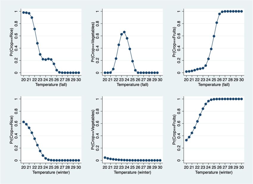
Agronomy 2021, 11, 369                                                                                            2 of 17

                               Drawn from nationally representative farm household data in Taiwan, the present
                         study aims at examining the effect of climate variables, including temperature and precip-
                         itation, on the production of the three most important staple foods: rice, vegetables and
                         fruits. The use of farm household data in Taiwan for climate change impact assessment is
                         relevant, since more than 98% of the 721,224 farm households who engaged in agriculture
                         production in Taiwan are growers of crops including rice, vegetables, fruits, specialty crops,
                         grains and other crops [29]. Examination of the effect of climate change on food production
                         in Taiwan can provide solid evidence and a significant complement to the existing body of
                         knowledge.
                               The contribution of the present study is three-fold. First, most of the country- or
                         region-specific studies in Asia are targeted at South Asian countries. Insufficient evidence
                         of the effect of climate change on Northeast Asian agriculture accentuates the need to
                         explore the impacts of climate change in the region. Second, one common characteristic of
                         most northeast Asian countries is their structure, with the majority of farms being small in
                         scale [30]. Taking Taiwan as an example, the average size of the farmland is approximately
                         1.02 hectares according to the most recent statistics. Empirical evidence supporting the
                         climate effect on Taiwan’s staple food production provides a significant complement to the
                         scant literature on the losses or gains of smallholder farms in their process of adaptation
                         to climate change. Third, Taiwan is characterized by clear spatial and seasonal variations
                         in temperature and rainfall. There are two distinct climatic characters on the island: “the
                         tropical monsoon climate in the south and subtropical monsoon climate in the north” [31].
                         This study, therefore, can advance our understanding of how the impact of climate change
                         varies with seasonal or spatial variability within a country.
                               The major research problem this study attempts to address is: What are the effects
                         of climate change on farm households’ production of staple foods of various kinds? To
                         this end, we base our analysis on the structural Ricardian model [32]. The Ricardian
                         or structural Ricardian models have been used to examine the effect of climate change,
                         addressing the production-related effects of current climatic conditions and a long-term
                         projection or simulation of the effect of climate change [27,28,33–42]. However, empirical
                         extensions to considering the cluster-correlated effect of climate on food production have
                         been limited. This study aims to bridge this knowledge gap by extending the structural
                         Ricardian model to accommodate for spatial clustering of the climate variables while
                         examining their effects on staple food production.
                               The remainder of this paper is as follows. Section 2 presents the spatial variations
                         in climate variables and the distribution of the three staple foods in Taiwan. Section 3
                         delineates the 2015 Census of Agriculture, Forestry, Fishery and Animal Husbandry data
                         (in short, 2015 Agriculture Census data) and the structural Ricardian model. Following
                         Section 3 are the results and discussion. The final section summarizes the major findings
                         and possible future extensions of the present research.

                         2. Spatial Distribution of Staple Foods and Climatic Variations
                               The spatial distribution of the three staple foods are different (Figure 1). Rice is more
                         concentrated in the coastal area of central and central-south counties. Among the top
                         three counties, the first two are located in central Taiwan while the third is located in the
                         south. The largest county in the central area, Nantou county, is an inland county which
                         takes a relatively small share of total rice production in Taiwan. Although vegetables are
                         also more concentrated in central Taiwan, the counties in the top club tend to be located
                         more in the south when compared to the top club of rice. Among the top three counties
                         producing vegetables, one is in the central area while the other two are in the south. The
                         spatial distribution of fruits is mainly concentrated in southern Taiwan. The top three
                         counties producing fruits are all in the south. A comparison of the spatial distribution of
                         rice, vegetables and fruits indicates a shift from north-central to central and south.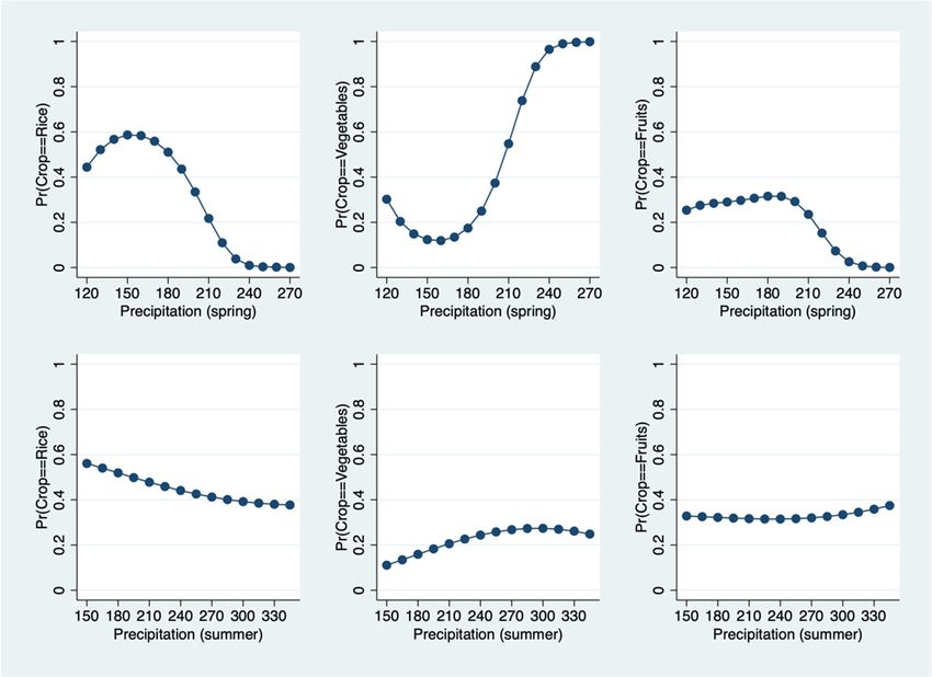
which is which
projectedis projected
to rise byto1.3–1.8
rise by°C1.3–1.8
under°C theunder the representative
representative concentration
concentration pathwaypathway
(RCP) 4.5(RCP) 4.5 scenario,
scenario, and may andreachmay
thereach thea high
high of of a°C3.0–3.6
3.0–3.6 surge °C surge
at the endatofthe end
this of this century
century
under anunder
RCP 8.5 an scenario
RCP 8.5 [43].
scenario [43]. On average,
On average, there is athere
mild is a milddifference
spatial spatial difference
in tempera‐in tempera‐
ture; the ture;
annual thetemperature
annual temperature in southern
in southern Taiwan isTaiwan
about 24 is about
and 2224°Cand 22 °C
in the in the
north north [31].
[31].
Agronomy 2021,In In to
11,contrast
369 contrast
the mild to spatial
the mild spatial variations
variations in temperature,
in temperature, the variations
the variations in precipitation
in precipitation are are 3 of 17
more obvious
more obvious (Figure 2). (Figure 2).
Figure Figuredistribution
Figure1.1.Spatial
Spatial 1. Spatial distribution
distribution ofrice,
of of rice, vegetables
rice,vegetables
vegetables fruits.and fruits.
andfruits.
and
Thebetween
temperature in Taiwan hasthe
been rising by about ◦ 1.3 seasonal
C in the variations
past
Taiwan
Taiwan lies lies
between the the Eurasian
Eurasian and and
the Pacific, andPacific,
thus and
the thus the
seasonal variations in 100 years,
in which
is projected to rise 1.3–1.8 ◦ C under the representative concentration pathway (RCP)
rainfall are mainly affected by the Siberian High and Pacific
rainfall are mainly affected by the Siberian High and Pacific Subtropical high and its ac‐ Subtropical high and its ac‐
4.5 scenario, andandmaysystem
reach the high ◦ C surge at the end of this century under
companyingcompanying
circulationcirculation
and weather weather [44]. Theof
system a 3.0–3.6
[44].
wet The
seasonwet inseason
Taiwan instarts
Taiwan starts from
from
an RCP
May to October,
May to October, 8.5
which is which scenario
followed [43].
is followed
by the dry On average,
by season, there
the dryuntil
season, is a mild
untilthe
l April spatial
l April difference
year. inyear.
the following
following temperature;
the annual temperature in southern Taiwan is about 24 and 22 ◦ C in the north [31]. In
During theDuring the drythe
dry season, season, theinrainfall
rainfall centralinand central and southern
southern Taiwan decreases
Taiwan decreases rapidly from
rapidly from
whereas contrast
October, October, whereas to the
there
there is still mild
is stillspatial
considerable variations
considerable
rainfall theinnorth
inrainfalltemperature,
in the
andnorth thethe
and
east of variations
east of the in
windward precipitation are
windward
side [45].side [45].more obvious (Figure 2).
Figure 2. Spatial climatic variations (left panel: temperature; right panel: rainfall).
Figure climatic
Figure 2. Spatial 2. Spatialvariations
climatic variations (left
(left panel: panel: temperature;
temperature; right
right panel: panel: rainfall).
rainfall).
Taiwan lies between the Eurasian and the Pacific, and thus the seasonal variations
in rainfall are mainly affected by the Siberian High and Pacific Subtropical high and its
accompanying circulation and weather system [44]. The wet season in Taiwan starts from
May to October, which is followed by the dry season, until l April the following year.
During the dry season, the rainfall in central and southern Taiwan decreases rapidly from
October, whereas there is still considerable rainfall in the north and east of the windward
side [45].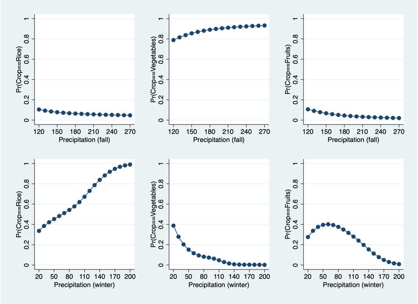
Agronomy 2021, 11, 369                                                                                               4 of 17

                              3. Materials and Methods
                              3.1. Data and Descriptive Statistics
                                   The data used in the present research are taken from the 1% sampling data from
                              the 2015 Agriculture Census data, which was recently released by the Executive Yuen in
                              Taiwan. According to the description of the Directorate General of Budget, Accounting and
                              Statistics [29], the 1% sampling data of the 2015 Agriculture Census is randomly sampled
                              from a total of 845,241 farm households, resulting in 6950 farm households in total. After
                              deleting the farm households whose major farm operation is livestock or who did not
                              engage in farming for land use, the data of farm households number 5315. We focus on
                              the farm households producing the three staple foods, rice, vegetables and fruits, which
                              comprise around 85% of the farm households producing mainly crops. According to the
                              codebook of 2015 Agriculture Census Survey, the fruits and vegetables included in the
                              two food groups are listed in Appendix A (Table A1). The final dataset contains a sample
                              size of 4487 farm households. Descriptions and descriptive statistics of the dependent and
                              explanatory variables are listed in Table 1. Note that most of the farm households produce
                              more than one crop; classification of the single staple food commodity is defined in terms
                              of the crop taking the largest share in total production value.

                                    Table 1. Variable definition and descriptive statistics.

             Variable                              Definition                                   Mean      Std Dev
             Outcome
                                Production value (National Taiwan Dollar, NTD,
        Production Value                                                                       3608.729    4836.03
                                       per unit farmland) of major crop
           Crop choice
              Rice                                Crop (rice)                                   0.459       0.50
           Vegetables                           Crop (vegetable)                                0.213       0.41
             Fruits                               Crop (fruit)                                  0.329       0.47
       Principal operator’s
          characteristics
              Male                    Gender of the principal operator                          0.806       0.40
              Age1                         Age (45–54 years old)                                0.050       0.22
              Age2                         Age (55–64 years old)                                0.198       0.40
              Age3                         Age (55–64 years old)                                0.299       0.46
              Age4                         Age (65–75 years old)                                0.250       0.43
              Age5                      Age (more than 75 years old)                            0.204       0.40
           Elementary             Education (elementary school and below)                       0.445       0.50
           Junior high                 Education (junior high school)                           0.236       0.42
           Senior high                 Education (senior high school)                           0.245       0.43
             College                   Education (college and above)                            0.073       0.26
              Exp1                   Farm experience (less than 5 years)                        0.090       0.29
              Exp2                 Farm experience (5 to less than 10 years)                    0.118       0.32
              Exp3                Farm experience (10 to less than 20 years)                    0.212       0.41
              Exp4                  Farm experience (more than 20 years)                        0.580       0.49
              Days1                   On-farm work (less than 60 days)                          0.417       0.49
              Days2                     On-farm work (60–149 days)                              0.381       0.49
              Days3            On-farm work (equal to or greater than 150 days)                 0.202       0.40
        HH (Household)
         characteristics
            HH size                      Household size (persons)                                3.664       2.06
           HH labor              Household members working on the farm (%)                      0.638       0.29
             Land                  Farmland used for crop production (are)                      76.739      89.02

                                  Due to high correlations of monthly climate data (Table 2), the seasonal averages in
                              temperature and precipitation are used to capture the effects of climate on crop choice and
                              production of the three staple food commodities. The four seasons are defined as: spring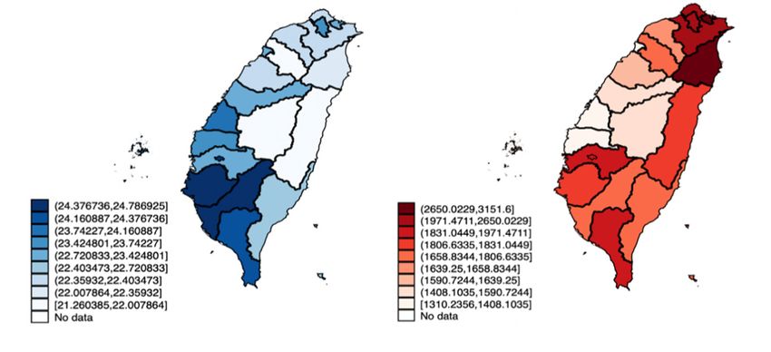
Agronomy 2021, 11, 369                                                                                                    5 of 17

                         (March, April, May), summer (June, July, August, September), fall (October, November)
                         and winter (December, January, February). It was indicated that summer is one month
                         longer than before in Taiwan [43]. Therefore, summer is composed of four months in the
                         present study.

                         3.2. Research Design
                              The effect of climate variables on staple food production is modeled in a two-stage
                         framework as in previous studies, for example, [33,34,38,40]. The two-stage modeling is
                         a generalization of the selection correction model [46]. In stage 1, the farm household’s
                         choice of a staple food to produce is based on the random utility theory and estimated
                         through a multinomial logit (MNL) model. The second stage incorporates the selection-bias
                         correction terms into the explanation of the production value of staple foods.
                              According to the random utility model [47,48], the choice of crop results from the
                         comparison of indirect utility associated with different choices by the decision unit, which
                         is the farm household in our case. There are three crops considered in this study: rice,
                         vegetable and fruit. Let the indirect utility associated with the choice of the mth crop be
                         denoted by Um  ∗ , where m = 1 denotes rice, m = 2 denotes vegetables and m = 3 denotes

                         fruits. The choice of the sth crop can be expressed as

                                                                    Us∗ >       max         ∗
                                                                                           Um                                (1)
                                                                            m=1,2,3,m6=s

                              Previous studies based on the Ricardian approach confirmed the influential role of
                         climate variables in crop choice, for example, [34,37,49,50]. The indirect utility is thus
                         further assumed to be a linear function of the characteristics of the farm, farm households
                         and principal operators as well as the climate variables
                                                        ∗
                                                       Um = Wαm + Xβm + ηm , m = 1, 2, 3                                     (2)

                              In the above equation, W and X are, respectively, the vector of climatic conditions and
                         the vector of socio-characteristics. αm and βm are the vectors of parameters and ηm is the
                         random disturbance terms. It is assumed that the difference in the indirect utility between
                         the crop chosen (s) and that not chosen (m 6= s) can be expressed as
                                                                               ∗ − U∗ )
                                                                    ε s = max(Um    s
                                                                         m6=s
                                                                                                                             (3)
                                                  = max(Wαm + Xβm + ηm − Wαs − Xβs − ηs )
                                                     m6=s

                                  According to (1), the difference between the indirect utility of crop choices defined in
                         (3) is less than zero, and the conditional probability of the choice of the sth crop is equal to
                         the conditional probability of negative utility difference.
                                  Following previous research, the choice of the three staple foods is basically unordered
                         in nature, and thus is estimated through the MNL model under the assumption that
                         (ε i1 , ε i2 , ε i3 ) follows a multinomial logistic distribution. Let the indicator variable, Ds , take
                         the value of 1 when the sth crop is chosen and 0 otherwise. The probability that the ith
                         farm operator chooses the sth crop can be expressed as

                                                                                   exp(Wαs + Xβs )
                                                Prob( Ds = 1 | X, W) =           3
                                                                                                                             (4)
                                                                                ∑m=1 exp(Wαm + Xβm )

                              The MNL model can be estimated through the following log-likelihood function:

                                                            N   3
                                                   L=    ∑∑         Dim · log[Prob( Dm = 1 | Xi , Wi )]                      (5)
                                                        i =1 m =1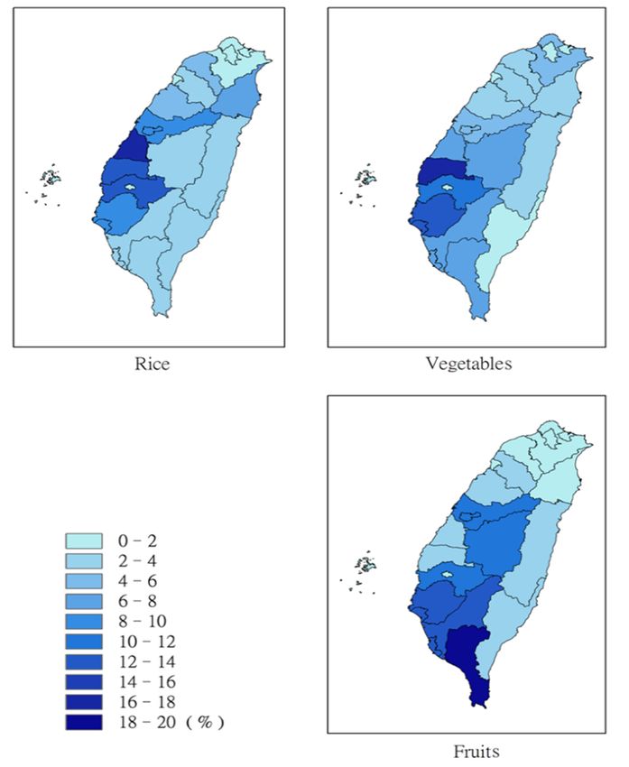
Agronomy 2021, 11, 369                                                                                                     6 of 17

                              Note that in the likelihood function in (5), the N observations are clustered into c
                         clusters for each of the climate variables to take into account the spatial correlation of the
                         observations located at the same cluster.
                              Possible correlation between crop choice and the production value of the crop is cor-
                         rected by including three selection correction terms into the production-value-determination
                         equation [47]. The effect of the climate variables on the production of the sth staple food
                         commodity is then estimated as the following

                                                                                3
                                                                                                  Pi · ln Pi

                                        E(Yi | Ds = 1) = Zi γs + Wc κs + σ ·   ∑       ri ·
                                                                                                   1 − Pi
                                                                                                             + ln Pm          (6)
                                                                               i 6=m

                         where Yi denotes the production value of the sth commodity produced by the ith farm
                         household, which is located in county c; Z is the explanatory variables affecting the
                         production value of the sth commodity other than the climate variables. The vectors of
                         parameters are denoted by γ and κ, respectively. It is important to note that there is
                         assumed independence across clusters (counties) but correlation within clusters (counties).

                         4. Results
                         4.1. The Choice of Crop Commodity
                               Coefficients for the stage 1 (MNL) model of the farm household’s choice of the three
                         staple foods are obtained through the estimation of the likelihood function specified in
                         Equation (5). Table 2 reports the estimates of the MNL estimate with the rice households as
                         the reference group while controlling for the climatic conditions and the socio-economic
                         characteristics of the principal operator or the farm household. The estimates of crop choice
                         reported in Table 2 are interpreted in a relative sense, i.e., the coefficient of one predictor
                         in the kth crop choice is a measure of the effect of the predictor on the probability of
                         choosing the kth crop over the reference group. We estimate two different specifications in
                         Table 2. The first four columns are the MNL model estimates, controlling only for seasonal
                         temperature and precipitation conditions.
                               The results in Table 2 are, in general, unsatisfactory, since only one coefficient is a
                         significant determinant of the choice of vegetables relative to rice. The last four columns
                         control for both the climatic conditions and the socio-economic characteristics of the
                         principal operator and the farm household. After controlling for the socio-economic
                         characteristics, the structural Ricardian model estimates are more satisfactory in terms of
                         the individual significance of the climate variables and their squared terms. Therefore,
                         in the following analysis, we calculated the selection correction terms according to the
                         estimates reported in columns 5 and 7 in Table 2.
                               According to the results in Table 2, the principal operator’s socio-economic charac-
                         teristics, including age, educational level, years of farming experience and on-the-farm
                         workdays, are important determinants for their choice of staple food commodities. Ad-
                         ditionally, seasonal average temperatures and their squared terms, and seasonal average
                         precipitation and their squared terms, are the major determinants of staple food production
                         in Taiwan. The results suggest the nonlinear effect of seasonal average temperature and
                         precipitation on the farm household’s choice of staple food commodity.
Agronomy 2021, 11, 369 7 of 17
Table 2. Maximum likelihood estimates of the multinomial logit (MNL) model.
Vegetables Fruits Vegetables Fruits
Variable
Coef. S.E. Coef. S.E. Coef. S.E. Coef. S.E.
Seasonal temp
Spring −5.5771 18.38 −20.8146 *** 2.95 −11.0578 13.98 −26.2727 *** 4.83
Summer 10.4691 9.92 −18.5363 *** 2.28 17.4990 ** 7.31 −12.8134 *** 3.15
Fall −7.5452 5.67 3.5163 *** 1.06 −8.0489 * 4.11 0.6089 2.40
Winter 10.7260 12.11 12.1159 *** 2.34 11.2718 8.97 14.3472 *** 3.46
Temperature sq
Spring 0.1546 0.44 0.5614 *** 0.08 0.2706 0.34 0.6885 *** 0.12
Summer −0.1775 0.15 0.2592 *** 0.03 −0.2784 ** 0.11 0.1684 *** 0.05
Fall 0.1071 0.12 −0.0017 0.03 0.0802 0.09 0.0302 0.05
Winter −0.3248 0.40 −0.4788 *** 0.08 −0.3206 0.29 −0.5292 *** 0.11
Seasonal
rainfall
Spring −0.0487 0.06 −0.1864 *** 0.01 −0.1200 *** 0.05 −0.2563 *** 0.03
Summer −0.0379 0.04 −0.0571 *** 0.01 −0.0354 0.03 −0.0655 *** 0.01
Fall 0.0035 0.01 0.0345 *** 0.00 0.0010 0.01 0.0302 *** 0.00
Winter 0.0540 0.07 0.0514 ** 0.02 0.0569 0.05 0.0877 ** 0.04
Rainfall sq
Spring 0.0001 0.00 0.0006 *** 0.00 0.0004 ** 0.00 0.0009 *** 0.00
Summer 0.0001 0.00 0.0001 *** 0.00 0.0001 0.00 0.0001 *** 0.00
Fall −0.0001 * 0.00 −0.0001 *** 0.00 0.0000 ** 0.00 −0.0001 *** 0.00
Winter 0.0000 0.00 −0.0002 *** 0.00 −0.0002 0.00 −0.0005 ** 0.00
Socio-economic
Male −0.1783 0.12 0.0807 0.07
Age2 −0.2635 0.18 −0.1297 0.16
Age3 −0.5095 ** 0.22 −0.4244 ** 0.18
Age4 −0.7505 *** 0.27 −0.5890 ** 0.25
Age5 −0.8833 *** 0.23 −0.5617 ** 0.25
Junior high 0.0591 0.12 0.1955 * 0.10
Senior high −0.2021 0.14 0.2049 0.14
College −0.4661 ** 0.18 0.0626 0.23
Exp2 0.0320 0.29 0.3142 0.23
Exp3 0.3825 * 0.20 0.1767 0.19
Exp4 0.2612 ** 0.13 0.3214 *** 0.11
Days2 0.9957 *** 0.21 0.9182 *** 0.30
Days3 2.1816 *** 0.32 2.0915 *** 0.36
Land −0.0029 *** 0.00 −0.0002 0.00
HH size 0.1052 ** 0.05 0.0806 ** 0.03
HH labor 1.0956 *** 0.39 1.0395 *** 0.34
_Cons −71.2235 177 356.805 43.57 −100.1176 134.95 358.1025 *** 65.41
No. of obs 955 1474 955 1474
Note: *, ** and *** denote significant at the 10%, 5% and 1% significance level.
4.2. Estimating the Structural Ricardian Model
Our stage 2 estimation of the structural Ricardian model incorporates the three
selection-correction terms into the clustered regression of the per-unit product value.
In this stage, the controlled variables include the social–economic characteristics of the
farm household and principal operator, seasonal temperatures and the squared terms, and
seasonal precipitations and the squared terms. The estimates of the clustered regression
conditioned on the farm household’s crop choice are reported in Table 3.
Coefficient estimates of the three selection-correction terms are significant for rice
farms but not significant for the other two staple food growers. Therefore, results from
uncorrected regression of the vegetable and fruit households are reported in columns 3–6
in Table 3. Based on the results in Table 3, seasonal temperatures and precipitations are
found to exhibit non-linear impacts on the production of each of the three staple foods.Agronomy 2021, 11, 369 8 of 17
Table 3. Clustered regression conditioned on choice of staple food commodity.
Rice Vegetables Fruits
Variable
Coef. Std. Err. Coef. Std. Err. Coef. Std. Err.
Seasonal temp
spring 99,667.82 * 50,650.42 57,722.10 37,019.12 8649.404 27,169.72
summer 64,089.40 * 31,053.26 29,068.89 19,671.57 13,578.69 15,010.17
fall −15,822.99 *** 4064.56 −57,617.96 *** 8740 −39,651.51 *** 7140.18
winter −45,873.56 26,783.95 −11,179.70 18,820.64 1160.545 17,882.19
Temperature sq
spring −2630.50 * 1332.38 −1279.33 875.01 −124.7959 681.49
summer −868.88 * 419.96 −493.95 * 280.6 −260.6547 226.6
fall 58.99 65.69 991.98 *** 214.3 719.5156 *** 156.83
winter 1834.12 * 1007.98 520.62 609.03 60.359 589.97
Seasonal rainfall
spring 941.71 * 495.53 −78.87 129.51 −116.4395 126.86
summer 242.24 * 125.04 −52.18 62.22 −69.60886 66.46
fall −130.16 ** 60.95 −43.50 ** 19.51 −21.9075 16.3
winter −377.69 ** 172.41 9.22 124.1 190.4126 * 102.68
Rainfall sq
spring −3.30 * 1.73 0.17 0.49 0.4660478 0.45
summer −0.49 * 0.26 0.10 0.11 0.1015217 0.13
fall 0.26 * 0.13 0.05 0.05 0.0248407 0.04
winter 2.10 ** 0.95 −0.02 0.32 −1.073143 ** 0.39
Selection terms
Rice −978.38 * 527.79
Vegetables −216.26 * 109.57
Fruits 1301.23 * 638.22
Control for
yes yes yes
socio-econ vars
_cons −1,468,703.00 * 757,124.10 −244,460.70 178,770.6 345,465.6
Note: *, ** and *** denote significant at the 10%, 5% and 1% significance level.
5. Discussion
The effect of the climate variables on the choice of major crop to produce is nonlinear,
since some of the coefficients for the squared terms are significant (Table 2). The coefficient
estimate from the MNL model is not a straightforward measure of the effects, especially
when there are squared terms involved. In order to provide a more intuitive description
of the impact of climatic conditions on the farm household’s crop choice, we present the
predictive margin plots by varying each of the climate variables over the whole dataset
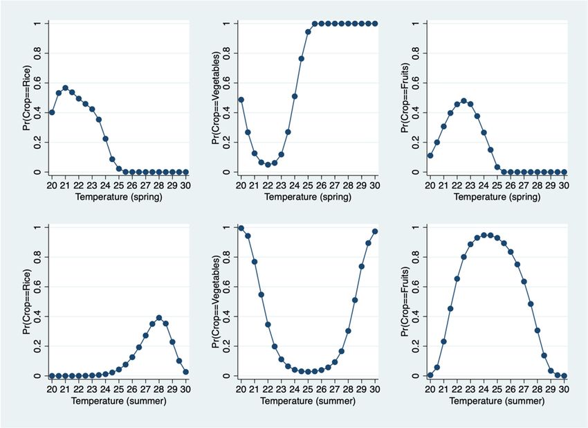
and calculate the averages of predicted probability for each crop choice. Figures 3 and 4
illustrate the effects of seasonal increases in temperature on the probability of crop choice.Agronomy 2021, 11, x FOR PEER REVIEW 9 of 17
to produce fruits when the temperature is below the average (27.74 °C) in summer. None‐
to produce
theless, fruits
when thewhen the temperature
temperature is higher is below
than the the average
average, (27.74
farm °C) in summer.
households None‐
will switch to
theless, when
Agronomy 2021, 11, 369 producing the temperature is higher than the average, farm households will switch
vegetables. Figure 4 illustrates the increasing tendency to produce fruits in the to 9 of 17
producing vegetables. Figure 4 illustrates the increasing
fall (upper panel) and in the winter (lower panel). tendency to produce fruits in the
fall (upper panel) and in the winter (lower panel).
Figure
Figure 3. Predictive
3. Predictive effect
effect of of temperature(spring,
temperature (spring,summer).
summer).
Figure 3. Predictive effect of temperature (spring, summer).
Figure 4. Predictive effect of temperature (fall, winter).
Figure
Figure 4. Predictive
4. Predictive effect
effect ofof temperature(fall,
temperature (fall,winter).
winter).
The upper panel of Figure 3 shows that farm households are inclined to produce veg-
etables when spring is warm. The average temperature in spring is 23.16 ◦ C; when it is 1 ◦ C
warmer, more than half of the farm household will choose to produce vegetables. However,
the lower panel of Figure 3 reveals that there is a higher probability of choosing to produce
fruits when the temperature is below the average (27.74 ◦ C) in summer. Nonetheless, when
the temperature is higher than the average, farm households will switch to producing
vegetables. Figure 4 illustrates the increasing tendency to produce fruits in the fall (upperAgronomy 2021, 11, 369 10 of 17
gronomy 2021, 11, x FOR PEER REVIEW 10 of 17
gronomy 2021, 11, x FOR PEER REVIEW 10 of 17
panel) and in the winter (lower panel).
The effects of seasonal average precipitations are graphed in Figures 5 and 6. Spring
The effects of seasonal average precipitations are graphed in Figures 5 and 6. Spring
and summer are the wet seasons in Taiwan. The upper panel of Figure 5 indicates that
The effects
and summer areofthe
seasonal average
wet seasons inprecipitations are graphed
Taiwan. The upper panel in
of Figures
Figure 55 indicates
and 6. Spring
that
increasing rainfall when it’s below the average level of 175 mm in the spring will increase
and summer
increasing are the
rainfall wetit’s
when seasons
belowintheTaiwan.
averageThe upper
level of 175panel
mm in of the
Figure 5 indicates
spring that
will increase
the farm household’s probability of producing rice. However, increasing precipitation at
increasing rainfall when
the farm household’s it’s belowofthe
probability average level
producing of 175 mmincreasing
rice. However, in the spring will increase
precipitation at
higher than
the farm household’s averageoflevels
probability in therice.
producing spring will eventually
However, increasinginduce the switch
precipitation at to vegetables.
higher than average levels in the spring will eventually induce the switch to vegetables.
higher than average levels in the spring will eventually induce the switch to vegetables.
Figure 5. Predictive effect of precipitation (spring, summer).
Figure 5. Predictive effect of precipitation (spring, summer).
Figure 5. Predictive effect of precipitation (spring, summer).
Figure 6. Predictive effect of precipitation (fall, winter).
Figure 6. Predictive effect of precipitation (fall, winter).
Figure 6. Predictive effect of precipitation (fall, winter).Agronomy 2021, 11, 369 11 of 17
The lower panel of Figure 5 nonetheless indicates that the probability of crop choice is
relatively stable relative to the increase in precipitation in the summer. Figure 6 portrays
the effect of increasing precipitation during the dry season (fall and winter) in Taiwan.
The choice of vegetables remains dominant in the fall (upper panel), while more rainfall
in the winter will persistently increase the farm household’s choice of producing rice
(lower panel).
In order to predict the effect of variations in climatic conditions on the production
value of the staple foods, we report the marginal effects of the climate variables in Table 4.
The F-statistic reported in Table 4 is the test for the joint significance of the seasonal
temperature (precipitation) and its squared term. According to the estimates reported in
Table 4, high temperature in the fall is found to have a unanimous dampening effect on the
production of staple foods, which is, in order, −$790 (vegetables), −$430 (rice) and −$50
(fruits). The results suggest the impacts of seasonal temperature variations in general vary
significantly across the staple food commodity chosen by the farm household. Among
the three staple food crops, vegetables seem to be more sensitive to seasonal variations
in temperature. There are two reasons that can explain this result. First, the growth
cycles of vegetables are generally shorter than rice and fruits, which may lead to more
sensitive responses of vegetables to seasonal temperature variations. Second, based on
the farm-household frequency distribution of major commodities in the 2015 Agriculture
Census data [51], we calculated the proportion of vegetable households producing mainly
leafy vegetables and found that the share of leafy vegetables was around 47%. Since leafy
vegetables are relatively more vulnerable to high/low temperatures, another reason to
explain why vegetables are more sensitive to temperatures is due to the fact that almost
half of the vegetable households produce mainly leafy vegetables.
Table 4. Predicted effects of temperature or precipitation on staple food production (USD per-unit farmland).
Commodity/ Temperature Precipitation
Season Mean Std. Dev. F-stat Mean Std. Dev. F-stat
Rice/
Spring −712.897 7.22 2.33 −8.135 * 0.19 3.61
Summer 522.128 1.57 2.16 0.604 * 0.06 3.75
Fall −432.440 *** 0.13 8.80 −3.274 ** 0.06 5.11
Winter 593.887 *** 4.23 9.01 −7.061 0.15 2.47
Vegetables/
Spring −2944.631 *** 38.49 9.45 −1.044 0.00 1.73
Summer 1163.105 3.82 0.96 −0.051 0.01 0.55
Fall −792.191 ** 0.87 4.48 −1.522 *** 0.01 8.53
Winter 2306.079 ** 26.45 4.77 0.596 0.00 0.05
Fruits/
Spring −278.334 4.26 2.15 1.528 0.03 2.29
Summer 45.317 0.12 0.16 −0.572 ** 0.02 6.02
Fall −46.642 ** 1.05 3.98 −0.594 0.00 1.4
Winter 351.390 4.18 0.19 4.495 ** 0.05 5.89
Note: 1 USD =30 NTD; *, ** and *** denote significant at the 10%, 5% and 1% significance level.
Taiwan is characterized by clear spatial variations and seasonal variations in rainfall.
Similar to the effect of variations in seasonal average temperature, the effect of seasonal
precipitation variations is found to vary significantly across the staple food commodity
chosen by the farm household. Nonetheless, our results indicate that increasing precipi-
tation in the winter can significantly increase the production of fruits which are heavily
concentrated in southern Taiwan.
A comparison of the three staple food commodities indicates that, among the three
staple foods, vegetable production is found to be affected by high temperatures to the
largest extent. Although the negative impact of high temperature in spring and fall may be
partly offset by the positive effect of higher temperature in winter, vegetables are the mostAgronomy 2021, 11, 369 12 of 17
vulnerable to the variations in seasonal average temperature among the three crops. As
for the effect of precipitation, we found that rice production is influenced to the greatest
extent, due to increasing precipitation in the spring.
To assess the impact of climate change on staple foods production, we perform
simulation analysis under four Representative Concentration Pathways (RCPs) scenarios.
The four scenarios in Table 5 (RCP2.6, RCP4.5, RCP6.0 and RCP8.5) are projected change in
climate parameters for Taiwan during the time period of 2021–2100, based on IPCC AR5
(the Fifth Assessment Report of the Intergovernmental Panel on Climate Change) [52].
Table 5. Scenarios of climate change.
Change in Temperature Change in Precipitation
Year Area
(◦ C) (mm)
RCP2.6 RCP4.5 RCP6.0 RCP8.5 RCP2.6 RCP4.5 RCP6.0 RCP8.5
2021–2040 North 0.64 0.68 0.61 0.78 41.1 47.1 36.6 78
Central 0.64 0.68 0.62 0.78 45.3 55.8 54.9 102.9
South 0.62 0.66 0.62 0.76 48.9 56.4 49.2 119.1
East 0.62 0.65 0.61 0.76 49.2 38.1 34.8 82.5
2041–2060 North 0.95 1.17 0.94 1.51 124.8 111.6 3.3 27.9
Central 0.93 1.15 0.94 1.5 127.8 123 −37.5 21.3
South 0.9 1.13 0.92 1.46 148.8 134.7 −222.3 22.5
East 0.91 1.13 0.91 1.46 120.6 104.4 −99.3 21.3
2061–2080 North 0.89 1.47 1.43 2.36 141.6 147.3 49.8 71.7
Central 0.88 1.45 1.43 2.32 147 152.1 69.3 83.1
South 0.86 1.41 1.40 2.27 142.2 150.9 68.4 99.6
East 0.86 1.41 1.39 2.27 128.4 125.1 60.3 70.2
2081–2100 North 0.77 1.57 1.98 3.16 154.8 108.9 125.4 49.8
Central 0.78 1.56 1.96 3.1 161.7 124.8 150 39.3
South 0.26 1.52 1.91 3.03 144.6 132.9 143.1 54.9
East 0.76 1.52 1.91 3.04 120.9 96.6 122.7 52.8
RCP2.6 is a scenario with global warming making very mild progress, and thus the
scenario with the least increase in temperature and the largest scale of rainfall increase. A
relatively modest progression of global warming is projected under RCP4.5 and RCP6.0.
Relatively speaking, RCP6.0 has a larger scale of temperature increase compared to RCP4.5,
especially in 2081–2100. On the other hand, precipitation is projected to increase steadily un-
der RCP4.5, whereas there is a decrease in precipitation, ranging from −37.5 to −222.3 mm
in 2041–2060, and a mild increase in the following two decades under RCP6.0. RCP8.5
is the scenario with the most severe progression in global warming. Under RCP8.5, the
temperature increases to the largest extent, while there seems to be some cyclical move-
ment in precipitation change among each 20-year interval. The increase in precipitation in
2021–2040 ranges from 78 to 119.1 mm, which is much larger in scale compared with the
21.3–27.9 mm precipitation change in 2041–2060. The increase in precipitation in 2061–2080
is back to the high in 2021–2040 with the increment ranges between 70.2 and 99.6 mm,
which then goes back to a mild change of 39.3–54.9 mm during 2081–2100. The projec-
tions in Table 5 reveals spatial variations in the change of temperatures and precipitations.
Central and northern Taiwan are projected to exhibit a larger-scale change in temperature,
whereas the central and southern areas have larger precipitation changes relative to the
north and the east.
Climate change impact assessment under the four scenarios are reported in Table 6.
The results indicate that climate change lowers the production value of rice under all four
scenarios with only three exceptions, which suggest the adverse effect of climate change on
rice production. As expected, there appear to be spatial differences in terms of the negative
effect of climate change on rice production. Central and southern Taiwan are projected to
experience more severe loss than in other parts of the island. Under RCP6.0, the adverseAgronomy 2021, 11, 369 13 of 17
effect of climate change on rice production reaches the high of approximately $2900 in the
last two decades of the century.
Table 6. Impacts of selected climate change scenarios (USD per-unit farmland).
Rice Vegetables Fruits
Year/Area Change in Production Value Change in Production Value Change in Production Value
RCP2.6 RCP4.5 RCP6.0 RCP8.5 RCP2.6 RCP4.5 RCP6.0 RCP8.5 RCP2.6 RCP4.5 RCP6.0 RCP8.5
2021–2040
North −753 −861 −672 −1416 −56 −66 −48 −124 246 278 222 435
Central −828 −1017 −999 −1861 −64 −84 −85 −175 266 320 311 556
South −892 −1027 −897 −2150 −72 −86 −73 −208 282 321 283 633
East −897 −700 −640 −1496 −73 −49 −44 −134 283 232 213 455
2041–2060
North −2258 −2028 −87 −543 −212 −176 33 8 674 626 83 244
Central −2311 −2231 642 −425 −219 −200 116 21 687 680 −115 211
South −2685 −2440 3945 −445 −262 −224 488 17 787 735 −1014 214
East −2181 −1898 1747 −423 −205 −163 239 19 651 588 −417 208
2061–2080
North −2556 −2675 −932 −1350 −248 −235 −40 −45 752 821 344 518
Central −2652 −2760 −1280 −1553 −260 −246 −79 −69 777 843 439 570
South −2566 −2737 −1263 −1846 −251 −245 −79 −105 752 834 433 647
East −2319 −2276 −1118 −1321 −223 −193 −63 −45 685 709 393 504
2081–2100
North −2788 −1992 −2299 −982 −280 −153 −169 34 807 642 751 469
Central −2912 −2275 −2737 −793 −294 −186 −220 52 841 718 869 413
South −2591 −2419 −2613 −1070 −281 −204 −208 18 721 755 832 484
East −2182 −1770 −2248 −1032 −212 −131 −167 23 642 578 733 475
Note: 1 USD =30 NTD.
With a few exceptions, climate change appears to have an adverse effect on the
production of vegetables, which are smaller in size compared to those for rice. There are
also spatial differences in the simulated effect of climate change on vegetable production.
Similar to rice, climate change impact on vegetables is larger in the northern and central
areas of Taiwan. There is a gradual increase in terms of the size of the negative effect under
RCP2.6 and RCP4.5. However, under RCP6.0 and RCP8.5, the effects of climate change
switch in signs during the entire time span. The impact of climate change on fruits are
different from the other two staple foods. The simulated results suggest that there is a
gradual increase in terms of the size of the effect on the production of fruits. Except for
RCP8.5, the positive impacts of climate change start with a size of around $210–$320 in
2021–2040, which later increase to approximately $640–$870 in the last two decades of
the century. Under RCP8.5, the effect of climate change first increases, but then decreases
in size.
The spatial differences in the simulated effect of climate change on the production of
the three staple foods are similar. The increment in or loss of production is larger in the
central and southern areas of Taiwan. Overall, it is found in this study that the effects of
climate change exhibit spatial and seasonal variations as in previous studies, for exam-
ple, [27,28]. This result is consistent with the finding in previous studies, example, [27,28].
Additionally, the present study confirms one more possible source of variations in climate
change impact, namely the variations across staple food commodities.
6. Conclusions
This study provides solid evidence and a significant complement to the existing body
of knowledge through the investigation of the effect of climate conditions on both crop
choice and subsequent production of the three most important staple foods. According to
the estimates from the structural Ricardian model, the impacts of seasonal temperature
variations are found to vary significantly across the staple food commodity chosen by theAgronomy 2021, 11, 369 14 of 17
farm household. Among the three staple food crops, vegetables seem to be more sensitive
to the seasonal variations in temperature. The effect of seasonal precipitation variations is
also found to vary significantly across the staple food commodities. Our results indicate
that increasing precipitation in the winter can significantly increase the production of fruits
which is heavily concentrated in southern Taiwan, whereas rice production is the most
sensitive to increasing precipitation in the spring.
Assessment of the impact of climate change under four RCP scenarios suggest the
adverse effect of climate change on the production of rice and vegetables. Most of the effect
of climate change, however, is positive for fruits. The simulated effect of climate change
under different RCP scenarios also suggest significant spatial differences in the impact of
climate change on the production of the three staple foods. Central and southern Taiwan
are projected to experience more severe loss in rice and vegetables production than in other
parts of the island.
Possible further exploration of the present work is two-fold. First, the use of adaptation
strategies other than crop choice or the use of combined coping strategies may resolve the
major limitation of this study. Second, some authors, for example, [53–55], indicated that
climate change impact assessment should also take the frequency and severity of extreme
climatic conditions into account. A possible extension of the present study is, therefore,
to explicitly acknowledge the effect of extreme weather or disaster loss in assessing the
impact of climate change.
Author Contributions: Conceptualization, Y.-H.L. and Y.-C.C.; methodology, Y.-H.L.; software, Y.-
H.L. and Y.-C.C.; validation, Y.-H.L.; formal analysis, Y.-H.L. and Y.-C.C.; investigation, Y.-H.L.;
resources, Y.-H.L.; data curation, Y.-H.L. and Y.-C.C.; writing—original draft preparation, Y.-H.L. and
Y.-C.C.; writing—review and editing, Y.-H.L.; visualization, Y.-H.L. and Y.-C.C.; supervision, Y.-H.L.;
project administration, Y.-H.L.; funding acquisition, Y.-H.L. All authors have read and agreed to the
published version of the manuscript.
Funding: Part of this research was funded by the Ministry of Technology and Science (MOST) in
Taiwan, grant number: MOST-106-2410-H-002-018. The APC was funded by the MOST project
undertaken by the author in the present.
Data Availability Statement: Publicly available datasets were analyzed in this study. The data can
be found here: https://www.stat.gov.tw/lp.asp?ctNode=6592&CtUnit=2393&BaseDSD=7&mp=4.
Conflicts of Interest: The authors declare no conflict of interest.
Appendix A
Table A1. Fruits and Vegetables.
Fruits Vegetables
Apple Persimmon Amaranth Ginger Pea
Avocado Pinang Asparagus Gracilaria Pea seedlings
Banana Pineapple Asparagus bean Green garlic Potato
Carambola Pitaya Aubergine Green onion Pumpkin
Citrus Plum Bamboo shoot Green soybean Radish
Gynura’s Deux
Coconut Plum flower Big stem mustard Spinach
Couleurs
Date palm Pomelo Bitter gourd Kale Sponge gourd
Grape sweetsop Burdock Kohlrabi Strawberry
Sweet potato
Guava Wax-jambos Cabbage Leaf mustard
leaves
Litchi Calabash (gourd) Leek Taro
Loquat Carrot Lettuce Tomato
Lungan Cauliflower Lotus root Water bambooAgronomy 2021, 11, 369 15 of 17
Table A1. Cont.
Fruits Vegetables
Mango Celery Lotus seed Water chestnut
Olive Celery cabbage Melon seeds Water nut
Other fruit Chillies Muskmelon Water spinach
Papaya Coriander Netted melon Watermelon
Parami Cucumber Onion Winter gourd
Passion fruit Fern Onion bulb Yellow daylily
Garland Oriental pickling
Peach Other fruits
chrysanthemum melon
Pear Garlic Pak-Choi (Bailey)
Table 2. Correlation coefficient of monthly temperature and precipitation.
Month Jan Feb Mar Apr May Jun Jul Aug Sep Oct Nov Dec
Jan 1 0.8698 0.9162 0.7584 −0.6321 0.3298 −0.155 0.0904 0.5398 0.9292 0.9111 0.9077
Feb 0.9846 1 0.9587 0.7775 −0.6569 0.3892 −0.097 0.1192 0.6651 0.8183 0.6767 0.9231
Mar 0.9039 0.9459 1 0.832 −0.6543 0.5015 −0.2304 −0.0205 0.5345 0.8501 0.7491 0.9647
Apr 0.89 0.9202 0.9444 1 −0.5808 0.5256 −0.1507 −0.2431 0.4705 0.6182 0.6002 0.8548
May 0.7752 0.8006 0.8093 0.9482 1 0.1046 −0.1262 −0.4045 −0.4363 −0.686 −0.6786 −0.5734
Jun 0.5929 0.5951 0.5663 0.761 0.9182 1 −0.5089 −0.5816 0.1048 0.1557 0.1359 0.5387
Jul 0.2225 0.2089 0.1489 0.3819 0.6366 0.8823 1 0.6763 −0.045 0.0658 −0.084 −0.2741
Aug 0.4087 0.3981 0.3413 0.5685 0.7856 0.9595 0.9735 1 0.3478 0.3115 0.1819 −0.134
Sep 0.6412 0.6581 0.6562 0.8511 0.9636 0.9501 0.7654 0.876 1 0.4863 0.374 0.5101
Oct 0.7966 0.8051 0.7917 0.9451 0.9804 0.8731 0.5801 0.7404 0.9567 1 0.9003 0.7971
Nov 0.8824 0.8935 0.8887 0.985 0.9643 0.8099 0.4645 0.6443 0.8995 0.9794 1 0.7333
Dec 0.9891 0.9901 0.9277 0.9162 0.7885 0.5701 0.173 0.3698 0.6486 0.812 0.8988 1
Note: Upper triangle reports correlation coefficient of monthly precipitation; lower triangle reports that of monthly temperature. Different
highlight colors represent correlations in different seasons—grey (winter), yellow (spring), blue (summer), green (fall).
References
1. Katz, R.W. Assessing the impact of climatic change on food production. Clim. Chang. 1977, 1, 85–96. [CrossRef]
2. White, J.W.; Hoogenboom, G.; Kimball, B.A.; Wall, G.W. Methodologies for simulating impacts of climate change on crop
production. Field Crops Res. 2011, 124, 357–368. [CrossRef]
3. Ahmed, K.F.; Wang, G.; Yu, M.; Koo, J.; You, L. Potential impact of climate change on cereal crop yield in West Africa. Clim. Chang.
2015, 133, 321–334. [CrossRef]
4. Famien, A.M.; Janicot, S.; Ochou, A.D.; Vrac, M.; Defrance, D.; Sultan, B.; Noël, T. A bias-corrected CMIP5 dataset for Africa using
the CDF-t method-A contribution to agricultural impact studies. Earth Syst. Dyn. 2018, 9, 313–338. [CrossRef]
5. Faye, B.; Webber, H.; Naab, J.B.; MacCarthy, D.S.; Adam, M.; Ewert, F.; Lamers, J.P.A.; Schleussner, C.F.; Ruane, A.; Gessner,
U.; et al. Impacts of 1.5 versus 2.0 ◦ C on cereal yields in the West African Sudan Savanna. Environ. Res. Lett. 2018, 13, 034014.
[CrossRef]
6. Mabhaudhi, T.; Nhamo, L.; Mpandeli, S.; Naidoo, D.; Nhemachena, C.; Sobratee, N.; Slotow, R.; Liphadzi, S.; Modi, A.T. The
water-energy-food nexus as a tool to transform rural livelihoods and wellbeing in southern Africa. Int. J. Environ. Res. Public
Health 2019, 16, 2970. [CrossRef]
7. Sultan, B.; Defrance, D.; Iizumi, T. Evidence of crop production losses in West Africa due to historical global warming in two crop
models. Sci. Rep. 2019, 9, 12834. [CrossRef]
8. Sultan, B.; Parkes, B.; Gaetani, M. Direct and indirect effects of CO2 increase on crop yield in West Africa. Int. J. Clim. 2019, 39,
2400–2411. [CrossRef]
9. Defrance, D.; Sultan, B.; Castets, M.; Famien, A.M.; Baron, C. Impact of Climate Change in West Africa on Cereal Production Per
Capita in 2050. Sustainability 2020, 12, 7585. [CrossRef]
10. Reynolds, M.; Ortiz, R. Adapting crops to climate change: A summary. In Climate Change and Crop Production; Reynolds, M.P., Ed.;
CAB International: Wallingford, UK, 2010; pp. 1–8.
11. Davis, C.L.; Vincent, K. Climate Risk and Vulnerability: A Handbook for Southern Africa, 2nd ed.; CSIR: Pretoria, South Africa, 2017;
p. 202.
12. Nhamo, L.; Matchaya, G.; Mabhaudhi, T.; Nhlengethwa, S.; Nhemachena, C.; Mpandeli, S. Cereal production trends under
climate change: Impacts and adaptation strategies in Southern Africa. Agriculture 2019, 9, 30. [CrossRef]Agronomy 2021, 11, 369 16 of 17
13. Mendelsohn, R.; Dinar, A.; Williams, L. The distributional impact of climate change on rich and poor countries. Environ. Dev.
Econ. 2006, 11, 159–178. [CrossRef]
14. Liu, J.; Folberth, C.; Yang, H.; Röckström, J.; Abbaspour, K.; Zehnder, A.J.B. A global and spatially explicit assessment of climate
change impacts on crop production and consumptive water use. PLoS ONE 2013, 8, e57750. [CrossRef]
15. Mendelsohn, R.; Massetti, E. The use of cross-sectional analysis to measure climate impacts on agriculture: Theory and evidence.
Rev. Environ. Econ. Policy 2017, 11, 280–298. [CrossRef]
16. Deressa, T.T.; Hassan, R.M. Economic impact of climate change on crop production in Ethiopia: Evidence from cross-section
measures. J. Afr. Econ. 2009, 18, 529–554. [CrossRef]
17. Wang, J.; Mendelsohn, R.; Dinar, A.; Huang, J.; Rozelle, S.; Zhang, L. The impact of climate change on China’s agriculture. Agric.
Econ. 2009, 40, 323–337. [CrossRef]
18. Masud, M.M.; Rahman, M.S.; Al-Amin, A.Q.; Kari, F.; Filho, W.L. Impact of climate change: An empirical investigation of
Malaysian rice production. Mitig. Adapt. Strat. Glob. Chang. 2012, 19, 431–444. [CrossRef]
19. Ahmad, A.; Ashfaq, M.; Rasul, G.; Wajid, S.A.; Khaliq, T.; Rasul, F.; Saeed, U.; ur Rahman, M.H.; Hussain, J.; Baig, I.A.; et al.
Cereal production in the presence of climate change in China. In Handbook of Climate Change and Agroecosystems; Rosenzweig, C.,
Hillel, D., Eds.; Imperial College Press: London, UK, 2015; pp. 219–258.
20. Bawayelaazaa Nyuor, A.; Donkor, E.; Aidoo, R.; Saaka Buah, S.; Naab, J.B.; Nutsugah, S.K.; Bayala, J.; Zougmoré, R. Economic
impacts of climate change on cereal production: Implications for sustainable agriculture in Northern Ghana. Sustainability 2016, 8,
724. [CrossRef]
21. Arshad, M.; Amjath-Babu, T.S.; Krupnik, T.J.; Aravindakshan, S.; Abbas, A.; Kächele, H.; Müller, K. Climate variability and yield
risk in South Asia’s rice–wheat systems: Emerging evidence from Pakistan. Paddy Water Environ. 2017, 15, 249–261. [CrossRef]
22. Mendelsohn, R.; Wang, J. The impact of climate on farm inputs in developing country agriculture. Atmosfera 2017, 30, 77–86.
[CrossRef]
23. Fahad, S.; Wang, J. Farmers’ risk perception, vulnerability, and adaptation to climate change in rural Pakistan. Land Use Policy
2018, 79, 301–309. [CrossRef]
24. Gao, J.; Mills, B.F. Weather shocks, coping strategies, and consumption dynamics in rural Ethiopia. World Dev. 2018, 101, 268–283.
[CrossRef]
25. Nahar, A.; Luckstead, J.; Wailes, E.J.; Alam, M.J. An assessment of the potential impact of climate change on rice farmers and
markets in Bangladesh. Clim. Change 2018, 150, 289–304. [CrossRef]
26. Chuang, Y. Climate variability, rainfall shocks, and farmers’ income diversification in India. Econ. Lett. 2019, 174, 55–61. [CrossRef]
27. Hossain, M.S.; Arshad, M.; Qian, L.; Zhao, M.; Mehmood, Y.; Kächele, H. Economic impact of climate change on crop farming in
Bangladesh: An application of Ricardian method. Ecol. Econ 2019, 164, 106354. [CrossRef]
28. Hossain, M.S.; Qian, L.; Arshad, M.; Shahid, S.; Fahad, S.; Akhter, J. Climate change and crop farming in Bangladesh: An analysis
of economic impacts. Int. J. Clim. Chang. Strateg. Manag. 2019, 11, 424–440. [CrossRef]
29. Directorate General of Budget, Accounting and Statistics. 2015 Agriculture, Forestry, Fishery and Animal Husbandry Census Report;
DGBAS: Taipei, Taiwan, 2017.
30. Shogenji, S.-I. Current position and future direction of agriculture in northeast Asia. In Food Security and Industrial Clustering in
Northeast Asia; Kiminami, L., Nakamura, T., Eds.; Springer: Tokyo, Japan, 2016; pp. 33–45.
31. Geography of Taiwan, The Climate of Taiwan. Available online: http://twgeog.ntnugeog.org/en/climatology/ (accessed on 8
November 2020).
32. Mendelsohn, R.; Nordhaus, W.D.; Shaw, D. The impact of global warming on agriculture: A Ricardian analysis. Am. Econ. Rev.
1994, 84, 753–771.
33. Kurukulasuriya, P.; Mendelsohn, R. Modeling Endogenous Irrigation: The Impact of Climate Change on Farmers in Africa; Policy
Research Working Paper; No. 4278; World Bank: Washington, DC, USA, 2007.
34. Kurukulasuriya, P.; Mendelsohn, R. Crop switching as a strategy for adapting to climate change. Afr. J. Agric. Resour. Econ. 2008,
2, 105–125.
35. Seo, S.N.; Mendelsohn, R.; Munasinghe, M. Climate change and agriculture in SriLanka: A Ricardian valuation. Environ. Dev.
Econ. 2005, 10, 581–596. [CrossRef]
36. Seo, S.N.; Mendelsohn, R. A Ricardian Analysis of the Impact of Climate Change on Latin American Farms; Policy Research Working
Paper; No. 4163; World Bank: Washington, DC, USA, 2007.
37. Seo, N.; Mendelsohn, R. Measuring impacts and adaptation to climate change: A structural Ricardian model of African livestock
management. Agric. Econ. 2008, 38, 151–165. [CrossRef]
38. Kurukulasuriya, P.; Kala, N.; Mendelsohn, R. Adaptation and climate change impacts: A structural Ricardian model of irrigation
and farm income in Africa. Clim. Chang. Econ. 2011, 2, 149–174. [CrossRef]
39. Chatzopoulos, T.; Lippert, C. Adaptation and climate change impacts: A structural Ricardian analysis of farm types in Germany.
J. Agric. Econ. 2015, 66, 537–554. [CrossRef]
40. Abidoye, B.O.; Kurukulasuriya, P.; Reed, B.; Mendelsohn, R. Structural Ricardian analysis of south-east Asian agriculture. Clim.
Chang. Econ. 2017, 8, 1740005. [CrossRef]
41. Etwire, P.M.; Fielding, D.; Kahui, V. Climate change, crop selection and agricultural revenue in Ghana: A structural Ricardian
analysis. J. Agric. Econ. 2019, 70, 488–506. [CrossRef]Agronomy 2021, 11, 369 17 of 17
42. Huong, N.T.L.; Bo, Y.S.; Fahad, S. Economic impact of climate change on agriculture using Ricardian approach: A case of
northwest Vietnam. J. Saudi Soc. Agric. Sci. 2019, 18, 449–457. [CrossRef]
43. National Science & Technology Center for Disaster Reduction. The Past and Future of Taiwan’s Climate; Research Center for
Environmental Changes Academic Sinica: Taipei, Taiwan, 2018.
44. National Science & Technology Center for Disaster Reduction. Climate Change in Taiwan: Scientific Report 2017. Physical Phenomena
and Mechanisms, General Summary; Research Center for Environmental Changes Academic Sinica: Taipei, Taiwan, 2018.
45. Central Weather Bureau, Climatic Characteristics of Seasonal Rainfall in Taiwan. Available online: https://www.cwb.gov.tw/
Data/service/hottopic/14277057430.pdf (accessed on 17 October 2020).
46. Dubin, J.; McFadden, D. An econometric analysis of residential electric appliance holdings and consumption. Econometrica 1984,
52, 345–362. [CrossRef]
47. McFadden, D. Conditional logit analysis of qualitative choice behavior. In Frontiers in Econometrics; Zarembka, P., Ed.; Academic
Press: New York, NY, USA, 1974; pp. 105–142.
48. Maddala, G.S. Limited-Dependent and Qualitative Variables in Econometrics; Cambridge University Press: New York, NY, USA, 1983.
49. Moore, M.; Negri, D. A multiple production model of irrigated agriculture applied to water allocation policy of the bureau of
reclamation. J. Agric. Resour. Econ. 1992, 17, 29–43.
50. Wang, J.; Mendelsohn, R.; Dinar, A.; Huang, J. How Chinese farmers change crop choice to adapt to climate change. Clim. Chang.
Econ. 2010, 1, 167–185. [CrossRef]
51. Directorate General of Budget, Accounting and Statistics. Farm Household Frequency Distribution of Major Commodities in the 2015
Agriculture, Forestry, Fishery and Animal Husbandry Census Survey; DGBAS: Taipei, Taiwan, 2017.
52. Taiwan Climate Change Projection Information and Adaptation Knowledge Platform. Available online: https://tccip.ncdr.nat.
gov.tw/index_eng.aspx (accessed on 17 October 2020).
53. Rosenzweig, C.; Iglesius, A.; Yang, X.B.; Epstein, P.R.; Chivian, E. Climate change and extreme weather events—Implications for
food production, plant diseases, and pests. Glob. Chang. Hum. Health 2001, 2, 90–104. [CrossRef]
54. Monirul, M.M.Q. Climate change and extreme weather events: Can developing countries adapt? Clim. Policy 2003, 3, 233–248.
55. Wang, S.L.; Ball, E.; Nehring, R.; Williams, R.; Chau, T. Impacts of Climate Change and Extreme Weather on U.S. Agricultural
Productivity: Evidence and Projection; NBER Working Paper; No. 23533; National Bureau of Economic Research: Cambridge, UK,
2017.You can also read