Estimating the phase volume fraction of multi phase steel via unsupervised deep learning
←
→
Page content transcription
If your browser does not render page correctly, please read the page content below
www.nature.com/scientificreports
OPEN Estimating the phase volume
fraction of multi‑phase steel
via unsupervised deep learning
Sung Wook Kim1, Seong‑Hoon Kang2, Se‑Jong Kim2* & Seungchul Lee1,3,4*
Advanced high strength steel (AHSS) is a steel of multi-phase microstructure that is processed under
several conditions to meet the current high-performance requirements from the industry. Deep
neural network (DNN) has emerged as a promising tool in materials science for the task of estimating
the phase volume fraction of these steels. Despite its advantages, one of its major drawbacks is its
requirement of a sufficient amount of training data with correct labels to the network. This often
comes as a challenge in many areas where obtaining data and labeling it is extremely labor-intensive.
To overcome this challenge, an unsupervised way of learning DNN, which does not require any manual
labeling, is proposed. Information maximizing generative adversarial network (InfoGAN) is used to
learn the underlying probability distribution of each phase and generate realistic sample points with
class labels. Then, the generated data is used for training an MLP classifier, which in turn predicts the
labels for the original dataset. The result shows a mean relative error of 4.53% at most, while it can be
as low as 0.73%, which implies the estimated phase fraction closely matches the true phase fraction.
This presents the high feasibility of using the proposed methodology for fast and precise estimation of
phase volume fraction in both industry and academia.
Automotive steel products are required to have good mechanical properties with high toughness and strength,
which are mainly accomplished by controlling the distributions of micro-constituents in steels. Numerous studies
have investigated the formulation of various steel microstructures based on parameters such as temperature, the
concentration of carbon, time, and thermomechanical processing, including heat treatments, cooling, anneal-
ing, etc. Nonetheless, only a few studies have been successful in the identification and quantification of micro-
structures, which is of paramount interest in the steel-making industry and academia. The separation of phases
becomes more challenging and ambiguous, as the number of micro-constituents gets larger due to the complex
characteristics of microstructures under different conditions. For example, complex micro-constituents can often
possess the same crystallographic arrangement but with varying degrees of defects in the c ells1, which makes it
difficult to distinguish between themselves.
The basic form of phase identification as well as the estimation of phase volume fraction consists of manually
counting the appearances of each micro-constituent through optical microscopy (OM) or scanning electron
microscopy (SEM). The so-called point counting methodology is often used as a reference in the literature1–4
for verifying if a proposed quantification method is appropriate. Even though it generally assures high accuracy
of the actual phase volume fraction, it is often limited in its usage for the enormous amount of time and a large
number of images necessary to obtain a 95% r eliability4,5.
Electron backscatter diffraction (EBSD) has recently become a widely used tool to make microstructural
classification of s teels1,2,6–8. EBSD offers several features, including image quality that allows us to show detailed
features of the microstructures such as the boundaries. It also allows phase identification by phase contrast pre-
sented from different diffraction intensities of each phase. As such, we also utilize EBSD images in this study to
extract raw training data. Wilson et al.9 distinguished martensite from ferrite simply using a threshold pattern
quality (PQ) value. Pixels with lower PQ than the threshold were classified as martensite, in another case as fer-
rite. However, the method is valid only when the PQ profile exhibits a clear bimodal distribution. Kang et al.1
proposed applying a grain-average function to process the PQ profile and unveil the dominant distribution peaks.
1
Department of Mechanical Engineering, Pohang University of Science and Technology, 77 Cheongam‑ro,
Pohang, Republic of Korea. 2Korea Institute of Materials Science, 797 Changwon‑daero, Seongsan‑gu, Changwon,
Republic of Korea. 3Graduate School of Artificial Intelligence, Pohang University of Science and Technology,
77 Cheongam‑ro, Pohang, Republic of Korea. 4Institute of Convergence Research and Education in Advanced
Technology, Yonsei University, 50 Yonsei‑ro, Seoul, Republic of Korea. *email: ksj1009@kims.re.kr; seunglee@
postech.ac.kr
Scientific Reports | (2021) 11:5902 | https://doi.org/10.1038/s41598-021-85407-y 1
Vol.:(0123456789)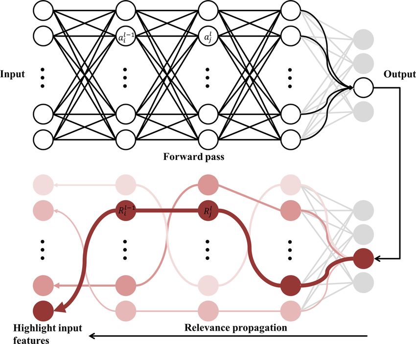
www.nature.com/scientificreports/
The author suggests extracting martensite from a ferrite matrix in DP steels using the average band contrast
and identifying bainite of TRIP steel with the local variations of band contrast and orientation inside a grain.
However, the study emphasizes the dependency of phase volume fraction on the user-defined definition angle
of grain boundary, which is the case for most EBSD-based identifications. Tomaz et al.2 presented an almost
identical phase fraction estimation on a low manganese HTP steel utilizing EBSD with a maximum fraction
difference of 5%, but the author also acknowledges criteria for separation would vary for different types of steels
and processing parameters.
Not only are EBSD-based methods unreliable for different types of steel and processing parameters, but they
are also labor-intensive. In recent years, such a disadvantage led to the development of numerous data-driven
techniques and studies3,10–13 along with the rise of machine learning. Gola et al.11 used a few data mining methods
such as standardization and successive backward elimination to pre-process raw data and made classification
by nonlinear SVM. The study achieved the classification accuracy of 87.15% on dual-phase steel consisting of
ferrite and martensite when used with feature elimination and standardization. Azimi et al.12 first demonstrated
an automated EBSD image labeling scheme using the deep learning-based image segmentation method reaching
the state-of-the-art classification accuracy of 93.94%. Bulgarevich et al.13 similarly demonstrated an automated
optical microscopy steel image labeling at pixel-level using a fast Random Forest statistical algorithm, which
showed a high percentage and location areas agreed between machine learning and manual examination results.
Though it is difficult to tell which result is the best due to unmatched test data and criteria for evaluation, high
accuracy was guaranteed only if there had been substantial manually labeled training data. In this sense, the ease
of implementation has not been enhanced significantly for data-driven methods than the traditional methods
for the estimation of phase volume fraction.
Therefore, we propose a novel means of estimating the phase volume fraction of multi-phase steel without the
manual labeling of phases, following an unsupervised manner. This is demonstrated by using a type of generative
model, InfoGAN to generate points of specific labels, followed by the training of Multi-layer Perceptron (MLP)
classifier using the generated sets. InfoGAN is an extension to vanilla generative adversarial network (GAN)
that allows for disentangled latent representation learning by training given input samples along with codes. The
disentangled latent representation allows for users’ control because unlike GAN, users can expect what samples
would be generated by controlling the codes to certain directions. To validate that our proposed model is appli-
cable for a wide range of AHSS alloys, six different types of steels with varying compositions of microstructures
are made and tested on it. The result shows that regardless of the chemical compositions, the model estimates the
phase volume fraction very well with the mean relative error of 0.73% at best. As far as we are concerned, this is
the first study on the quantification of multi-phase steel based on unsupervised deep learning.
The rest of the paper is broken down as follows. “Revision of recent generative deep learning techniques”
provides a recap on the related deep learning techniques encountered in this study whilst “Methodology” details
the proposed methodology. The experimental result is discussed in “Results and discussion” and finally, the paper
is concluded in “Conclusion”.
Revision of recent generative deep learning techniques
Generative adversarial network (GAN). Since its first advent as a novel framework of a generative
model, GAN14 has stimulated an explosion of related works in the deep learning community especially for gen-
erating realistic images of human beings, animals, objects, and backgrounds. GAN is known to learn data dis-
tributions implicitly, which is why it can often be very powerful in imitating the distributions. It is composed
largely of two components, a generative model G that captures the data distribution and a discriminator D that
figures out whether or not a sample came from the training data. GAN is frequently referred to as a minimax
game since the two models compete against each other for simultaneous optimization. Both models are usually
differentiable multilayer perceptrons. The ultimate goal of the algorithm is to reach the equilibrium state in
which the probability of D is equal to 0.5. The objective function is as follows:
min max V (D, G) = Ex∼Pdata (x) [log(D(x))] + Ez∼Pz (z) [log(1 − D(G(z)))] (1)
G D
As few weaknesses of GAN (e.g., mode collapse) were reported, numerous variants of GAN have been
introduced in addition to various training t echniques15 that made it possible to solve the issues. Information
maximizing generative adversarial network (InfoGAN) is one that fixes the problem of learning entangled latent
representation.
Information maximizing generative adversarial network (InfoGAN). InfoGAN16 is an extension
to GAN, which can learn disentangled latent representation in an unsupervised manner. Disentangled repre-
sentation allocates a separate set of dimensions for each salient attribute that is informative for distinguishing
data of different categories. Learning in such a way brings an advantage over the traditional GAN in that it can
control what to output. This is made possible by having an extra term in the objective function, which maximizes
the mutual information between an observation and a latent variable during training. InfoGAN decomposes the
input noise vector into two parts that are denoted by z , a source of noise, and c , a latent code. The latent code
c represents the salient attributes or the semantic features of the data distribution. The objective function of
InfoGAN is as follows:
min max V (D, G) = V (D, G) − I(c, G(z, c)) (2)
G D
Mutual information between the latent code c and the generated sample is denoted by I(c, G(z, c)). The
intuitive interpretation of mutual information is the reduction of uncertainty in c when G(z, c) is observed. By
Scientific Reports | (2021) 11:5902 | https://doi.org/10.1038/s41598-021-85407-y 2
Vol:.(1234567890)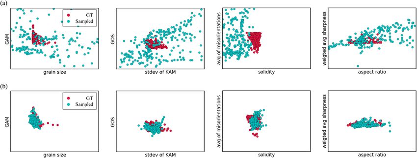
www.nature.com/scientificreports/
Figure 1. The workflow of the proposed method.
maximizing it, the model will be trained so that c and generated samples are relevant to each other. In reality,
however, the computation of the term is costly because of posterior P(c|x)16. suggests estimating it using a lower
bound by replacing the posterior with an auxiliary distribution Q(c|x) for approximation, a technique known as
Variational Information Maximization17.
I(c, G(z, c)) =H(c) − H(c|G(z, c))
=Ex∼G(z,c) Ec′ ∼P(c|x) [logP(c ′ |x)] + H(c)
(3)
=Ex∼G(z,c) DKL (P(·|x)||Q(·|x)) + Ec′ ∼P(c|x) logQ(c ′ |x) + H(c)
′
≥Ex∼G(z,c) Ec′ ∼P(c|x) logQ c |x + H(c)
′
By treating H(c) as a constant and using the formula Ex∼X,y∼Y |x f (x, y) = Ex∼X,y∼Y |x,x ′ ∼X|y [f (x , y)], a
variational lower bound LI (G, Q) of mutual information is defined as follows:
LI (G, Q) =Ec∼P(c),x∼G(z,c) logQ(c|x) + H(c)
=Ex∼G(z,c) Ec′ ∼P(c|x) [logQ(c ′ |x)] + H(c) (4)
≤I(c, G(z, c))
In Eq. (3), it is notable that as the auxiliary distribution Q becomes similar to the true distribution P , the lower
bound becomes closer to the mutual information term. Hence, the maximal mutual information is achieved
when the lower bound attains its maximum LI (G, Q) = H(c). To conclude, the objective function of InfoGAN
can be rewritten as follows:
min max VInfoGAN (D, G, Q) = V (D, G) − LI (G, Q) (5)
G,Q D
The intuition behind the InfoGAN model is to find an auxiliary distribution Q that changes G(z, c) to the right
c and at the same time, a generator G that generates the right G(z, c) so that Q operates well.
Methodology
General workflow. The overall workflow of the proposed method is illustrated in Fig. 1. It is largely divided
into two parts. The first part in which InfoGAN is trained using unlabeled raw data is named unsupervised
learning. This corresponds to Phase I of Fig. 5. The next part in which an MLP classifier is trained to learn a deci-
sion boundary and predict labels on the raw data is named supervised learning. This corresponds to Phase II of
Fig. 5. Lastly, the phase volume fraction is estimated by summing up the areas of the identically labeled samples.
Estimation of phase volume fraction. In this study, six different types of steels with varying composi-
tions of microstructures were built for both training and testing. Figure 2 shows examples of EBSD images.
Table 1 shows the underlying microstructures that make up each type of steel and its proportions while Table 2
shows the chemical composition of each steel.
As shown in Table 2, the steels can be divided largely into two different sets. The first set of steels (A, B, C, and
D) differs from the second set of steels (E and F) in that a different combination of chemical composition was
intentionally formed to create a scenario where the sets come from statistically different distributions. Each steel
was constructed under different processing conditions. To estimate the true phase fraction of Steel A, B, C, and
D, a quench-type dilatometer (Dilatronic III, Theta Inc.) was used and the dilatometric strain is plotted against
temperature as shown in Fig. 3. For Steel E and F, JMatPro was used. Before any measurement, a specimen was
heated with an induction coil in a vacuum, and a Pt-PtRh (Type R) thermocouple was attached to its surface to
measure the temperature and dilatometric data at the same time18.
A dilatometer measures the thermal expansion strain of a specimen during a heat cycle. If a phase transforma-
tion occurs leading to a change in the thermal coefficient, there will be an inflection in the dilatometric curve,
Scientific Reports | (2021) 11:5902 | https://doi.org/10.1038/s41598-021-85407-y 3
Vol.:(0123456789)
www.nature.com/scientificreports/
Figure 2. EBSD band contrast (BC) images of different steels. (a–f) corresponds to Steel A—F in the alphabetic
order. Pixel size of images are 1592 by 1196.
Ferrite Bainite Pearlite Martensite Remarks
Steel A 0.0 0.0 0.0 100.0 Single phase
Steel B 9.52 0.0 0.0 90.48 Dual phase
Steel C 9.52 90.48 0.0 0.0 Dual phase
Steel D 9.52 35.5 0.0 54.98 Triple phase
Steel E 2.0 4.3 0.1 93.4 Quadruple phase
Steel F 5.7 22.8 0.5 70.9 Quadruple phase
Table 1. Six types of steels with varying compositions of microstructures (all units are in percentage).
Steel C Si Mn
A, B, C, D 0.24 1.50 1.15
E, F 0.42 0.16 0.60
Table 2. Chemical composition of each steel (all units are in wt%).
which indicates the start of the transformation. As shown in Fig. 3, Steel A is cooled down to room temperature
at the rate of 100◦ C per second. Steel B had the slope of the dilatometer curve unchanged until the transforma-
tion to a specific phase when it was cooled down from 820◦ C to room temperature. This indicates it is composed
of ferrite and another phase. We could assume that the phase other than ferrite was martensite by calculating
the transformation temperatures using the given empirical formula19. For calculating the formula, the chemical
composition of the austenite phase at transformation is assumed equal to the chemical compositions of the raw
material and of the austenite in the two-phase equilibrium since the change in slope of cooling curve before phase
transformation is unclear. To be specific, based on the formula, the MS temperatures turned out to be 403◦ C
and 369◦ C for Steel A and B respectively. As the measured transformation temperatures (396◦ C and 358◦ C)
turned out to be lower than the calculated ones and the transformation was fast (please refer to Figure S2 in Sup-
plementary Information for transformation speed), we decided the phase was martensite. The proportion of the
two phases was estimated using SEM images of etched specimens by labeling the percentage of the bright regions
as ferrite and the dark regions as martensite. For the case of Steel C, it was cooled down from 820 to 400◦ C and
left there for 10 min before it was cooled down again. Since Steel C and D saw no transformation of austenite to
ferrite during the cool down above 400◦ C, they were considered to have the same amount of ferrite as Steel B. We
knew that bainite was created because the transformations at 400◦ C occurred at a higher temperature than the
calculated MS temperature of Steel B, and they happened at a relatively slower pace. To estimate the percentage
Scientific Reports | (2021) 11:5902 | https://doi.org/10.1038/s41598-021-85407-y 4
Vol:.(1234567890)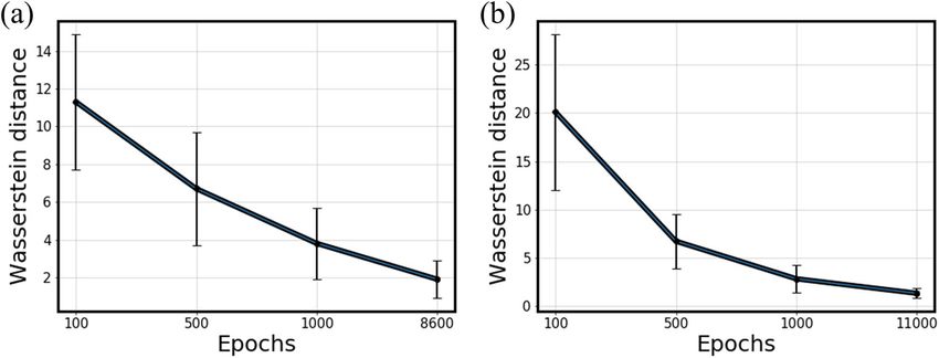
www.nature.com/scientificreports/
Figure 3. Dilatation curve plot.
Figure 4. Examples of segmented EBSD images by grain (Steel D). Pixel size of the leftmost image is 90 by 86.
of bainite in the steels, the ratio of dilatation by bainite transformation during a 12-s hold (l1) to dilatation by
the transformation of austenite to bainite at 400◦ C (l2) was multiplied by the percentage of austenite. No residual
austenite was observed for any of the aforementioned process conditions. Further details regarding the estimation
of phase ratio are provided in Supplementary Information (Figure S1, S2). Process conditions for Steel E and F
are listed in Table S1. The dilatation curve plot of Steel E and F is not provided.
Description of extracted features. By using TIMS software developed by Korea Institute of Materials
Science, we analyzed and extracted 19 features from each segmented EBSD image shown in Fig. 4. It should
be noted that the images of different pixel sizes were segmented using the software based on grain boundary.
The description of the features is summarized in Table 3. Some of the features include grain size (diameter),
grain average misorientation (GAM), the standard deviation of KAM, solidity, area-weighted average sharpness,
etc. They are commonly considered to be the main contributive factors to distinguish different microstructural
classes in many works of literature1,4,6,8,11, though there exists no rule-of-thumb for which one is more impor-
tant than another in distinctive cases. For an intuitive understanding of some of the features, further details are
provided in Supplementary Information (Table S2). The training data consists of 116,811 samples without any
labels. Although the true phase fraction of each steel is known in advance from observing the dilatometer curve,
labels for each grain on the EBSD images are left to be discovered by the proposed method in this study. 20% of
raw data was used as a test set.
p is the number of pixels in a grain. s is the step size. g is user-defined kernel and k is the number of kernel
elements. Ai denotes the area of an image while Ac is the area of convex hull image.w and h are weight and height
of grain respectively. wi = d × D/2, where d and D are distance and convexity depth. I represents luminance.
Implementation of deep learning. For the implementation of deep learning, we used Python 3.5.2 and
Keras 2.2.5. For training, a GPU (RTX 2080) was used for fast computation. In this study, 1D InfoGAN was
implemented because the type of training data is numerical (a single row in the table corresponds to 19 extracted
feature values for one segmented image). Training a GAN model is often difficult due to the stochasticity of its
nature. For training images, the traditional method is to output the generated sample image, compute the evalua-
tion scores20, and save the current model for every pre-defined epochs. This allows the user to check if the gener-
ated sample is realistic (to the eyes of the beholder) and use the saved GAN model of the same epoch. Training a
1D GAN is particularly challenging in some aspects because, unlike images, there exists no established method
to visualize high-dimensional data to effectively monitor the ongoing training status of the GAN model. There-
fore, an alternative is to monitor an appropriate evaluation score and visualize as many data distributions as
possible. Here, L2 reconstruction error was used as the evaluation measure, and four different combinations of
Scientific Reports | (2021) 11:5902 | https://doi.org/10.1038/s41598-021-85407-y 5
Vol.:(0123456789)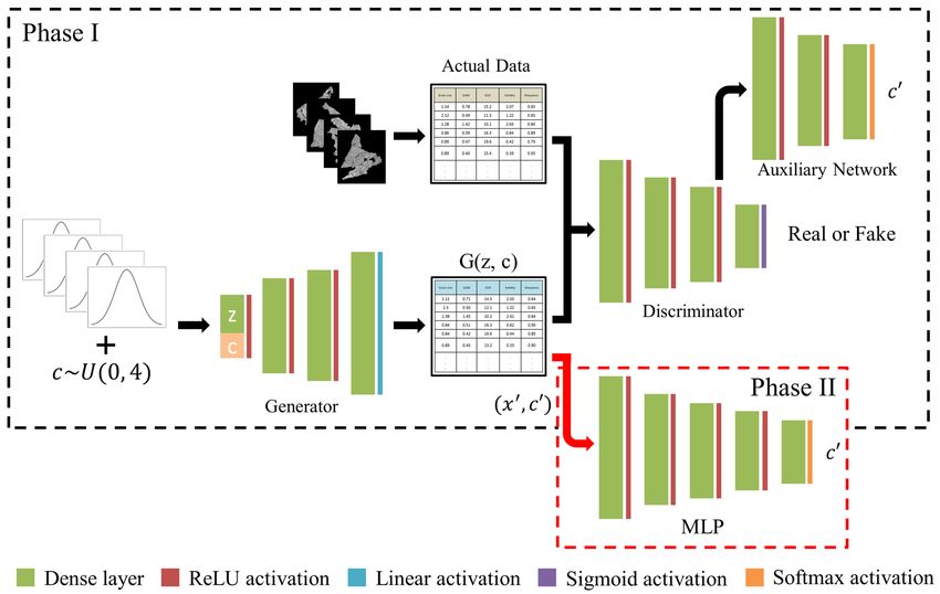
www.nature.com/scientificreports/

                                                    Input feature                                                                     Symbol and description

                                             1      Grain size                                                                        ds = 2 ×
                                                                                                                                                 p×s2
                                                                                                                                                  π
                                             2      GAM

                                                                                                                                                          i KAMi
                                                                                                                                      GAM =                p
                                                                                                                                                                                −1
                                             3      Std. of KAM

                                                                                                                                                                        g(i,j) g(i+x,j+y)
                                                                                                                                      σKAM , KAM (i,j) =                       k
                                                                                                                                                              −1
                                             4      GOS

                                                                                                                                                      i gave gi
                                                                                                                                      GOS =                p
                                             5      Solidity                                                                          S=     Ai
                                                                                                                                             Ac
                                             6      Avg. of misorientations at the boundary                                           µmis
                                             7      Aspect ratio                                                                      AR =        w
                                                                                                                                                  h
                                             8      Weighted avg. sharpness

                                                                                                                                                          i wi ×sharpness i                   D
                                                                                                                                      µsharp =                               , sharpness =   d
                                                                                                                                                                 i wi
                                             9      Avg. band contrast in the grain                                                   µBC =       Imax −Imin
                                                                                                                                                  Imax −Imin
                                             10     Std. of band contrast within the grain                                            σBC
                                             11     Area weighted avg. grain size of neighbor grains surrounding the current grain    µGS
                                             12     Area weighted avg. GAM of neighbor grains surrounding the current grain           µGAM
                                             13     Area weighted avg. std. of GAM of neighbor grains surrounding the current grain   µσ GAM
                                             14     Area weighted avg. GOS of neighbor grains surrounding                             µGOS
                                             15     Area weighted avg. aspect ratio of neighbor grains surrounding                    µAR
                                             16     Area weighted avg. band contrast of neighbor grains surrounding                   µnBC
                                             17     Area weighted avg. std. of band contrast of neighbor grains surrounding           µσ nBC
                                             18     Area weighted avg. solidity of neighbor grains surrounding                        µS
                                             19     Area weighted avg. sharpness of neighbor grains surrounding                       µnS

                                            Table 3.  Description of input features.

                                            Figure 5.  InfoGAN and MLP classifier structures are shown inside dashed black and   ′
                                                                                                                                     red
                                                                                                                                     ′
                                                                                                                                          boxes, respectively. In
                                            Phase I, InfoGAN is trained. In Phase II, the generator creates samples and labels (x , c ) that are given as input
                                            to MLP for training. Then, the trained model performs the classification of raw data.

          Scientific Reports |   (2021) 11:5902 |                    https://doi.org/10.1038/s41598-021-85407-y                                                                                   6

Vol:.(1234567890)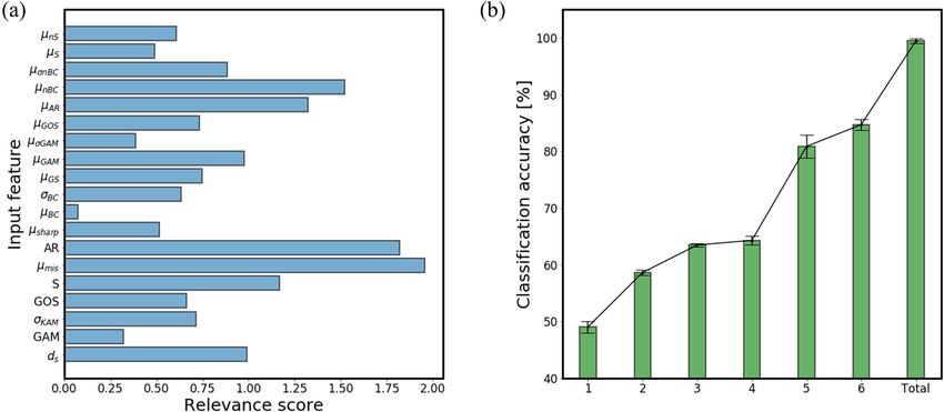
www.nature.com/scientificreports/

                                   Generator network (G)                     Discriminator network ( D)               Auxiliary network (Q)
                                   Layer       Type              Dimension   Layer      Type              Dimension   Layer      Type              Dimension
                                               Latent ( z) + Code
                                   Input                          4+4        Input      Feature           19          Input      Hidden layer      50
                                               (c)
                                               Dense layer       50                     Dense layer       100                    Dense layer       50
                                   Hidden 1                                  Hidden 1                                 Hidden 1
                                               ReLU activation   –                      ReLU activation   –                      ReLU activation   –
                                               Dense layer       50                     Dense layer       50                     Dense layer       20
                                   Hidden 2                                  Hidden 2                                 Hidden 2
                                               ReLU activation   –                      ReLU activation   –                      ReLU activation   –
                                               Dense layer       19                     Dense layer       1                      Dense layer       4
                                   Output                                     Output    Sigmoid activa-               Output     Softmax activa-
                                               Linear activation –                                                                                 –
                                                                                        tion                                     tion

                                  Table 4.  The proposed InfoGAN structure. Each network holds two hidden layers but with a varying number
                                  of nodes. Input to the auxiliary network is the output of the second hidden layer in the discriminator.

                                  2D graphs were plotted to monitor the data points being generated. The reconstruction error is equivalent to the
                                  mean squared error between the training samples and generated samples. It was computed for every 100 epochs
                                  and displayed while playing the minimax game, as stated in Eq. (5). Given a generator G and a set of training data
                                  X = {x1 , x2 , x3 , . . . , xn }, the reconstruction error is defined by:
                                                                                                  n
                                                                                             1
                                                                             Lrec (G, X) =      ||G(z, c) − xi ||2                                         (6)
                                                                                             n
                                                                                               i=1

                                      As mentioned in “Revision of recent generative deep learning techniques”, the structure of InfoGAN is
                                  similar to that of an ordinary GAN except for a few extensions due to the latent code c . Figure 5 illustrates the
                                  structure of InfoGAN and that of an MLP of which the training procedure is indicated as a black and a red arrow,
                                  respectively. They are also presented as Phase I and II, respectively because they are two separate models and are
                                  not trained simultaneously by sharing a loss function. Phase II comes after Phase I. To elaborate, after Phase I
                                  (training InfoGAN) is over, what is created by the generator with labels is given as input to the MLP for training
                                  (Phase II). In Phase I, a Gaussian noise matrix z concatenated with random latent code c is given as input to
                                  the generator, hence the representation G(z, c) for the generator output. The generator is an MLP with an input
                                  layer, two hidden layers and an output layer the size of the total feature counts. Similarly, the discriminator is
                                  an MLP with an input layer, two hidden layers, but   ′
                                                                                          with two output layers, one for the discrimination and the
                                  other for the control variable or the latent code c . For each output layer, binary cross-entropy and categorical
                                  cross-entropy were adopted respectively for computing loss. Inputs to the discriminator are both raw data x and
                                  generated sample G(z, c).
                                      For training the aforementioned InfoGAN model, He initializer was used to initialize the weights in the hid-
                                  den layers. Implementing Adam optimizer, the learning rate was set to 2e−4 while the exponential decay set to
                                  0.5. Hyper-parameters, including the number of epochs and batch size were set to 30,000 and 512, respectively.
                                  The dimension of the latent code depends on the prior knowledge of the number of classes of raw data. Training
                                  the generator and the discriminator was practiced one at a time, meaning that while updating the weights of
                                  the generator, the discriminator was not trained and vice versa. The proposed architecture of the InfoGAN for
                                  the case of Steel E is summarized in Table 4. Since Steel E is an example of a quadruple phase, the latent code
                                  with a dimension of four is appended to the latent space z , which was heuristically determined to have the same
                                  dimension. ReLU activation function is applied to the networks after every dense layer except for the output
                                  layers to account for the nonlinearity in the training data. However, different activation functions are utilized
                                  after the output layers depending on the purposes of each network. For example, the auxiliary network has a
                                  softmax activation function because it is required to output multiple labels.
                                      When the training of InfoGAN is completed, the generator is capable of sampling points from learned data
                                  distributions of a specified control variable. For instance, since Steel C had been known before to be dual-phase,
                                  it was trained to have′ two
                                                            ′
                                                               distinct data distributions from which the generator later sampled points. Then, the
                                  generated samples (x , c ) are provided as input to an MLP classifier, as shown in Phase II. After scaling the data
                                  from 0 to 1, the dataset was split into a train and a test set at a ratio of 8–2. The MLP classifier consists of an
                                  input layer of 19 dimensions, three hidden layers, and an output layer with the size depending on the number
                                  of classes of the steel in concern. For all steels, the test accuracy turned out above 99%, implying the models
                                  have been optimized. Last but not least, the raw data which had been used to train InfoGAN is put through the
                                  optimized feed-forward classifier network to give out the labels. The estimated phase fraction of each steel is
                                  presented in “Sec10”.

                                  Results and discussion
                                  Estimation of phase volume fraction. The result summarized in Table 5 implies the high feasibility of
                                  using the proposed method for a fast phase fraction estimation for steels or even any other materials without
                                  labeling all the training data. Though none of the estimated values is the same, all of them are on the right track
                                  as the models can distinguish the big and small chunks. The mean relative error for the estimations implies the
                                  high feasibility of using the proposed method. It shows that the mean relative error can reach at most 4.53%

Scientific Reports |   (2021) 11:5902 |                    https://doi.org/10.1038/s41598-021-85407-y                                                          7

                                                                                                                                                        Vol.:(0123456789)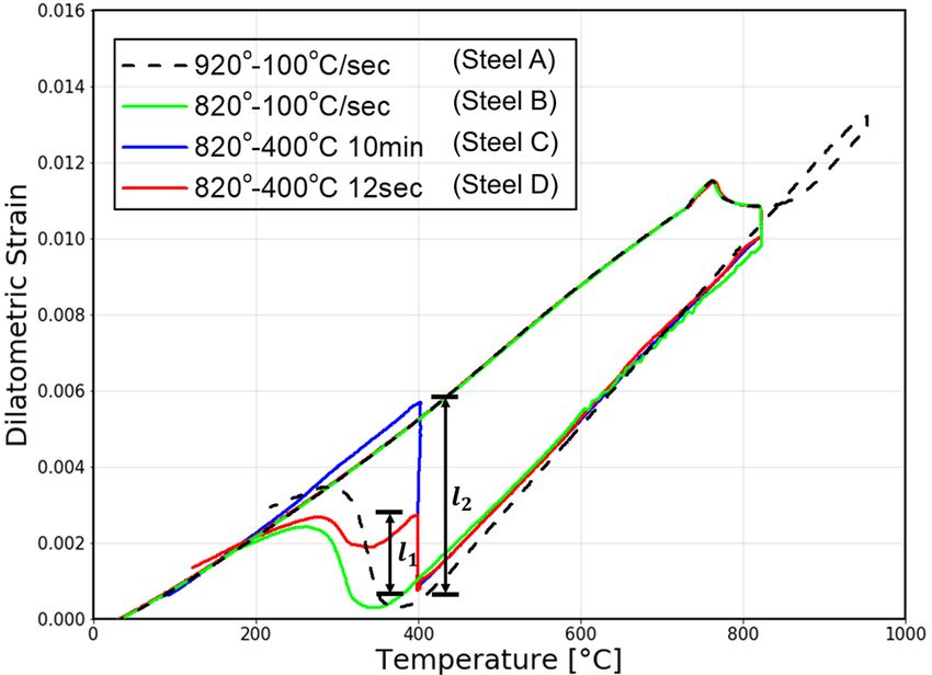
www.nature.com/scientificreports/

                                                            Ferrite     Bainite   Pearlite   Martensite   Relative ERROR
                                             Steel A
                                             True PF         0.0         0.0      0.0        100.0
                                                                                                          1.87
                                             Estimated PF    2.1         0.0      0.7         97.2
                                             Steel B
                                             True PF         9.5         0.0      0.0         90.5
                                                                                                          3.18
                                             Estimated PF    2.7         0.0      0.7         96.6
                                             Steel C
                                             True PF         9.5        90.5      0.0          0.0
                                                                                                          2.2
                                             Estimated PF   11.7        88.3      0.0          0.0
                                             Steel D
                                             True PF         9.5        35.5      0.0         55.0
                                                                                                          4.53
                                             Estimated PF   10.4        28.7      0.0         60.9
                                             Steel E
                                             True PF         2.0         4.3      0.1         93.4
                                                                                                          0.73
                                             Estimated PF    2.0         3.4      0.0         94.6
                                             Steel F
                                             True PF         5.7        22.8      0.5         70.9
                                                                                                          3.1
                                             Estimated PF    5.5        17.2      0.2         77.2

                                            Table 5.  True and estimated phase fraction of each type of steel (all units are in percentage).

                                            Figure 6.  (a) Sampled points at epoch 100 for Steel E. (b) Sampled points at epoch 11,000 for the same steel.
                                            The ground truth is shown in red dots while the sampled points are in green dots.

                                            while it can be as low as 0.73%, which is very close to the exact estimation. Furthermore, the result implies the
                                            proposed method is suitable for steels with different kinds of chemical compositions (Steel A, B, C, D, and Steel
                                            E, F). It is also inspirational in the sense that no domain knowledge of steel processing is necessary to estimate
                                            the phase fractions.
                                                Figure 6 shows an intuitive form of visualizing the data distributions, which demonstrates the gradual change
                                            in the form of distributions as optimization proceeds. The optimized InfoGAN models were stored during train-
                                            ing by screening both the L2 reconstruction error and the data distributions. Here, the red dots are the ground
                                            truths for Steel E, while the green dots are the sampled points at the specified epochs. It can be seen from (a) and
                                            (b) that as the model gets optimized, sampled points get closer to the ground truth meaning that they eventually
                                            come from more similar underlying data distributions. Not all results are shown for clarity.
                                                Table 6 compares the relative errors of the proposed approach with a number of baseline clustering models,
                                            showing that it outperforms them for the estimation of phase volume fraction in all steels. These models are
                                            composed of pure clustering models such as k-means, Gaussian mixture model (GMM), and density-based spatial
                                            clustering of applications with noise (DBSCAN) and combinations of various dimension reduction techniques
                                            and DBSCAN. For the combinations, the dimension reduction techniques are principal component analysis
                                            (PCA), autoencoder, and GAN that are denoted as P-, A-, and G- respectively. DBSCAN was selected as the sole
                                            clustering model after dimension reduction because of its superior result compared to the other two models.

          Scientific Reports |   (2021) 11:5902 |                     https://doi.org/10.1038/s41598-021-85407-y                                              8

Vol:.(1234567890)
www.nature.com/scientificreports/
Steel A Steel B Steel C Steel D Steel E Steel F Mean (%)
Relative error (%)
K-means 4.8 35.8 6.8 14.8 28.5 20.4 18.5
GMM 5.2 21.4 6.8 6.5 24.1 22.0 14.3
DBSCAN 2.8 8.5 8.3 6.8 19.6 3.1 8.2
P-DBSCAN 2.8 6.2 6.8 6.4 10.6 5.5 6.3
A-DBSCAN 1.9 8.7 4.3 8.7 1.3 3.0 4.7
G-DBSCAN 1.9 8.8 5.7 8.0 1.9 3.1 4.9
InfoGAN 1.9 3.2 2.2 4.5 0.7 3.1 2.6
Table 6. Comparison of the proposed approach with baseline clustering models. Best results presented in bold
font.
Figure 7. (a) PDFs for Steel E. (b) PDFs for Steel F. The ground truth is shown in a red curve while the
estimated PDF is in a black curve.
This implies that the proposed method is so far the most preferable choice for the phase classification of steels
in an unsupervised manner.
Evaluation of the fraction estimation. For evaluation, the probability density function was plotted at
four different epoch points to monitor if the learned data distribution was getting close to the ground truth as
the training progressed. The probability density function (PDF) was approximated by kernel density estimation
(KDE) or Parzen-Rosenblatt window method, which is a non-parametric way to estimate the PDF of a random
variable21. In statistics, it makes an inference about the population based on a finite data sample by applying
Gaussian kernels with a pre-defined bandwidth. Suppose (x1 , x2 , . . . , xn ) are i.i.d. samples drawn from a distribu-
tion with an unknown density f . The kernel density estimator is defined as follows:
n n
1 1 x − xi
fˆh (x) = Kh (x − xi ) = K (7)
n nh h
i=1 i=1
In Eq. (7), K represents a kernel, and h is a smoothing parameter or the bandwidth. Its intuitive meaning is
that normal kernels on each of the data points are summed to make the final kernel density estimate. For the
computation, a built-in Pandas module was used, and we set the smoothing parameter h to 0.6.
Figure 7 shows the plotted PDFs at four different epoch points for Steel E and F. Looking at the plots, the red
line represents the ground truth PDF, whereas the black line represents the estimated PDF. As the epoch number
increases, the estimated PDF becomes similar to the ground truth. At the final epochs, the PDFs almost overlap,
indicating that much similar data distributions have been learned by the models.
Besides, Wasserstein Distance (WD)22 was measured to quantify how similar two probability distributions are.
Figure 7 demonstrates how similar the learned distributions are to the ground truths for only a few features. It is
necessary to evaluate the overall similarity for all features combined. Averaging out WDs for all features solves
this problem. Figure 8 presents the gradual decrease in average WDs for Steel E and F as training progressed.
It can be concluded that the data distributions were learned similarly for all features, not just for the few ones.
Scientific Reports | (2021) 11:5902 | https://doi.org/10.1038/s41598-021-85407-y 9
Vol.:(0123456789)www.nature.com/scientificreports/
Figure 8. Average Wasserstein Distances at different epochs. (a) Steel E. (b) Steel F.
Epochs
100 500 1000 Best
Average Wasserstein distance
Steel A 14.15 ± 4.27 6.25 ± 2.86 3.57 ± 1.54 1.48 ± 0.47
Steel B 16.82 ± 6.31 3.21 ± 1.26 2.38 ± 1.19 1.16 ± 0.41
Steel C 7.79 ± 1.87 1.52 ± 0.47 0.89 ± 0.29 0.76 ± 0.19
Steel D 8.88 ± 2.20 2.20 ± 0.97 1.62 ± 0.82 0.77 ± 0.22
Steel E 11.28 ± 3.65 6.74 ± 3.00 3.81 ± 1.85 1.91 ± 1.01
Steel F 20.14 ± 8.08 6.65 ± 2.81 2.84 ± 1.37 1.27 ± 0.53
Table 7. Summary of average Wasserstein distances at different epochs.
Table 7 summarizes it for the rest of the steels. In the table, ‘Best’ indicates the epoch point for which each model
had the best performance (the least reconstruction error).
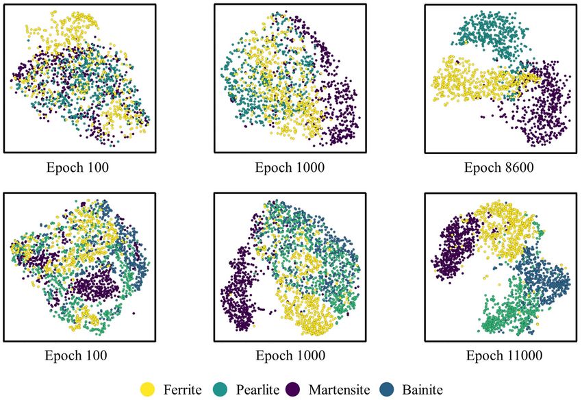
Figure 9 shows the feature visualizations using t-SNE23–26 on the InfoGAN generated features for Steel E and
Steel F. t-SNE is a widely used technique for visualizing high-dimensional data into 2D or 3D by projecting data
into a low dimensional space so that the clustering in the high-dimensional space is preserved. It measures the
similarity on a t-distribution of each point in data based on the distance of points and clusters them based on the
similarity scores. For its iterative optimization, the Kullback Leibler divergence of the distributions in both high-
dimension and low-dimension is minimized. In Fig. 9, the top row represents the embedded feature distributions
for Steel E while the bottom row does it for Steel F. The noteworthy part of it is that as the optimization gradually
reaches the minimum, the features representing each phase become distinctively separable from one another.
This implies the fact that at the optimal point, the model is capable of distinguishing the unique characteristics
of each feature and thus create similar points from the learned distributions.
Feature importance of input features. In many engineering fields, it is often extremely helpful to know
which features turned out to be critical for making the phase classification. Highlighting the input features a deep
learning model uses to support its prediction has been an essential part of explainable artificial intelligence27–30.
Though several techniques31–33 have been introduced to unveil the underlying mechanism of a deep neural
network, one of the most promising ones nowadays is the Layer-wise Relevance Propagation (LRP)34 which we
adopted in this study. When computing the amount of contribution that each input makes to the output of a
neural network, it can be denoted as the partial derivative of the output with respect to the input.
d
∂f
f (x) = f (a) + |x=a (x − a) + ǫ (8)
∂xp
p=1
As shown above, the second term of the Taylor s eries35 in its first-order with the higher-order terms repre-
sented as ǫ can be understood as describing the change in the output f (x) as xp varies. For the LRP technique, an
appropriate ‘a’ is searched so that the first and the higher-order terms erases out, leaving f (x) = di=1 Ri where
Ri is the relevance score interpreted as the contribution score.
The formula can be reformulated as follows for
any given two consecutive layers in a deep neural network: i Ri = j Rj . This is equivalent to a conservation
property, where what has been received by a neuron must be redistributed to the lower layer in an equal a mount34.
Figure 10 illustrates the general process of the LRP.
Scientific Reports | (2021) 11:5902 | https://doi.org/10.1038/s41598-021-85407-y 10
Vol:.(1234567890)www.nature.com/scientificreports/
Figure 9. t-SNE visualization of generated features at different epochs. The top row represents the embedded
feature distributions for Steel E while the bottom row does it for Steel F.
In LRP, the prediction output of a neural network propagates backward based on the trained weights and
biases, and the relevance score is calculated by Eq. (9):
(l−1) (l)
(l−1)
ai wij (l)
Ri =
j
(l−1) (l) Rj (9)
a
i i w ij
(l−1) (l−1) (l)
Ri is the relevance score of the ith node in (l − 1th) layer. ai is the activation value while wij denotes
the trained weights from the MLP. The weighted sum in the denominator is to ensure that the conservation
property holds.
In this study, the significance of input features is investigated for Steel D that constitutes the most evenly
distributed phase ratios. Of the three phases that constitute the steel, we focus on the classification of martensite
that has the largest ratio. Since we present the feature importance using only the LRP technique, we hereby
acknowledge the lack of evidence for the following result given solely by the data-driven method, and would
like to suggest the important design parameters for further study. Figure 11 (a) is a bar chart that shows the
relevance scores assigned to each input feature. The top three high scoring features are µmis , AR , and µnBC in the
sequential order, which is the average of misorientations at the boundary, aspect ratio, and the area-weighted
average band contrast of neighbor surrounding grains, respectively. It can be inferred from the result that they
should be considered as a priority when designing the composition of the micro-constituents in steel. We verify
the result by comparing various scenarios where a different number of high-scoring features are utilized to make
phase classification. Figure 11b shows how the elimination of a different set of input features affects the general
classification performance of MLP. Keeping the entire features provided the best classification accuracy of 99.5%
on average. Whereas using the six top features for training resulted in only a 14.8% reduction in accuracy, using
the single top feature had a much larger drop of 50.4%. This implies what has been labeled as more contributive
by the LRP technique is in fact, more important in the decision-making.
Conclusion
In this study, the estimation of phase volume fraction of multi-phase steel via unsupervised deep learning is
presented. To the best of our knowledge, it is the first time to solve the problem via unsupervised deep learning,
no longer requiring the tedious job of labeling data. The proposed method suggests a generalized approach to
Scientific Reports | (2021) 11:5902 | https://doi.org/10.1038/s41598-021-85407-y 11
Vol.:(0123456789)www.nature.com/scientificreports/
Figure 10. Schematic diagram showing the general process of LRP. Starting from the output from a trained
MLP, the relevance score is distributed backward. The input feature from the leftmost layer that is assigned the
highest relevance score is colored in dark red.
Figure 11. (a) Relevance score bar chart of input features of Steel D. (b) Comparison of scenarios where ‘Total’
keeps the entire features while the numbers (1–6) in the x-axis represent the number of high-scoring features
utilized for phase classification.
Scientific Reports | (2021) 11:5902 | https://doi.org/10.1038/s41598-021-85407-y 12
Vol:.(1234567890)www.nature.com/scientificreports/
identify and quantify the classes of multi-phase steel, revealing the possibility for even non-experts without any
prior knowledge to do the task. In total, six different types of steel with varying microstructure compositions were
tested. The result shows the estimated phase fractions to be a good match with the true phase fractions for all tests.
Furthermore, it implies the proposed method is suitable for steels with different kinds of chemical compositions
(Steel A, B, C, D, and Steel E, F). This is made possible by implicitly learning the data distribution similar to that of
the training data by using a type of a generative model, InfoGAN. An optimized generator is then able to output
a paired dataset controlled by the latent code specified by the user. Next, an MLP classifier is trained using the
generated dataset and performs a prediction on the raw data to provide them with labels. Several visualization
techniques including t-SNE were implemented to validate the aptness of the utilized InfoGAN model. Lastly, the
significance of input features is assessed by using LRP. We hope that this work can contribute to making a leap
forward in the automation of phase quantification that has previously been a laborious task. We also believe the
proposed method can be widely incorporated in the industries as well as the laboratories for research purposes.
Data availability
The datasets generated during and/or analyzed during the current study are available from the corresponding
author on reasonable request.
Received: 14 December 2020; Accepted: 1 March 2021
References
1. Kang, J.-Y. et al. Phase analysis of steels by grain-averaged EBSD functions. ISIJ Int. 51, 130–136 (2011).
2. Tomaz, R. F. et al. Complex phase quantification methodology using electron backscatter diffraction (EBSD) on low manganese
high temperature processed steel (HTP) microalloyed steel. J. Mater. Res. Technol. 20, 20 (2019).
3. Bulgarevich, D. S., Tsukamoto, S., Kasuya, T., Demura, M. & Watanabe, M. Pattern recognition with machine learning on optical
microscopy images of typical metallurgical microstructures. Sci. Rep. 8, 2078 (2018).
4. Zhao, H., Wynne, B. & Palmiere, E. A phase quantification method based on EBSD data for a continuously cooled microalloyed
steel. Mater. Charact. 123, 339–348 (2017).
5. Testing, A. S. f. & Materials. ASTM E562-11: Standard Test Method for Determining Volume Fraction by Systematic Manual Point
Count (Springer, 2011).
6. Zaefferer, S., Romano, P. & Friedel, F. EBSD as a tool to identify and quantify bainite and ferrite in low alloyed Al TRIP steels. J.
Microsc. 230, 499–508 (2008).
7. Wu, J., Wray, P. J., Garcia, C. I., Hua, M. & DeArdo, A. J. Image quality analysis: A new method of characterizing microstructures.
ISIJ Int. 45, 254–262 (2005).
8. Shrestha, S. L. et al. An automated method of quantifying ferrite microstructures using electron backscatter diffraction (EBSD)
data. Ultramicroscopy 137, 40–47 (2014).
9. Wilson, A., Madison, J. & Spanos, G. Determining phase volume fraction in steels by electron backscattered diffraction. Scripta
Mater. 45, 1335–1340 (2001).
10. Velichko, A. Quantitative 3D characterization of graphite morphologies in cast iron using FIB microstructure tomography. Adv.
Eng. Mater. 9, 39–45 (2009).
11. Gola, J. et al. Advanced microstructure classification by data mining methods. Comput. Mater. Sci. 148, 324–335 (2018).
12. Azimi, S. M., Britz, D., Engstler, M., Fritz, M. & Mücklich, F. Advanced steel microstructural classification by deep learning meth-
ods. Sci. Rep. 8, 2128 (2018).
13. Bulgarevich, D. S., Tsukamoto, S., Kasuya, T., Demura, M. & Watanabe, M. Automatic steel labeling on certain microstructural
constituents with image processing and machine learning tools. Sci. Technol. Adv. Mater. 20, 532–542 (2019).
14. Goodfellow, I. et al. Generative adversarial nets. Adv. Neural Inf. Process. Syst. 20, 2672–2680 (2014).
15. Salimans, T. et al. Improved techniques for training gans. Adv. Neural Inf. Process. Syst. 20, 2234–2242 (2016).
16. Chen, X. et al. Infogan: Interpretable representation learning by information maximizing generative adversarial nets. Adv. Neural
Inf. Process. Syst. 20, 2172–2180 (2016).
17. Barber, D. & Agakov, F. V. The IM algorithm: A variational approach to information maximization. Adv. Neural Inf. Process. Syst.
20, 201–208 (2003).
18. Kim, S.-J. et al. Development of a dual phase steel using orthogonal design method. Mater. Des. 30, 1251–1257 (2009).
19. Andrews, K. Empirical formulae for the calculation of some transformation temperatures. J. Iron Steel Inst. 20, 721–727 (1965).
20. Borji, A. Pros and cons of gan evaluation measures. Comput. Vis. Image Underst. 179, 41–65 (2019).
21. Hall, P. & Marron, J. On the amount of noise inherent in bandwidth selection for a kernel density estimator. Ann. Stat. 20, 163–181
(1987).
22. Arjovsky, M., Chintala, S. & Bottou, L. Wasserstein gan. arXiv :1701.07875 (Preprint) (2017).
23. van der Maaten, L. & Hinton, G. Visualizing data using t-SNE. J. Mach. Learn. Res. 20, 2579–2605 (2008).
24. Van der Maaten, L. & Hinton, G. Visualizing non-metric similarities in multiple maps. Mach. Learn. 87, 33–55 (2012).
25. Van Der Maaten, L. Learning a parametric embedding by preserving local structure. Artif. Intell. Stat. 20, 384–391 (2009).
26. Van Der Maaten, L. Accelerating t-SNE using tree-based algorithms. J. Mach. Learn. Res. 15, 3221–3245 (2014).
27. Swartout, W. R. & Moore, J. D. Second Generation Expert Systems 543–585 (Springer, 1993).
28. Montavon, G., Samek, W. & Müller, K.-R. Methods for interpreting and understanding deep neural networks. Digit. Signal Process.
73, 1–15 (2018).
29. Baehrens, D. et al. How to explain individual classification decisions. J. Mach. Learn. Res. 11, 1803–1831 (2010).
30. Samek, W., Wiegand, T. & Müller, K.-R. Explainable artificial intelligence: Understanding, visualizing and interpreting deep learning
models. arXiv :1708.08296 (Preprint) (2017).
31. Ribeiro, M. T., Singh, S. & Guestrin, C. Model-agnostic interpretability of machine learning. arXiv :1606.05386 (Preprint) (2016).
32. Yosinski, J., Clune, J., Nguyen, A., Fuchs, T. & Lipson, H. Understanding neural networks through deep visualization. arXiv
:1506.06579(Preprint) (2015).
33. Dosovitskiy, A. & Brox, T. in Proceedings of the IEEE Conference on Computer Vision and Pattern Recognition. 4829–4837.
34. Montavon, G., Binder, A., Lapuschkin, S., Samek, W. & Müller, K.-R. Explainable AI: Interpreting, Explaining and Visualizing Deep
Learning 193–209 (Springer, 2019).
35. Dienes, P. The Taylor Series: An Introduction to the Theory of Functions of a Complex Variable (Dover, 1957).
Scientific Reports | (2021) 11:5902 | https://doi.org/10.1038/s41598-021-85407-y 13
Vol.:(0123456789)www.nature.com/scientificreports/
Acknowledgements
This work was supported by the National Research Foundation of Korea (NRF) [Grant no. 2020R1A2C1009744];
Institute for Information communications Technology Promotion (IITP) [Grant no. 2019-0-01906]; Artificial
Intelligence Graduate School Program (POSTECH); Fundamental Research Program of the Korea Institute of
Materials Science [Grant no. PNK7760].
Author contributions
Formal analysis, investigation, methodology, writing—original draft, writing—review and editing, S.W.K.; con-
ceptualization, data curation, S.H.K.; supervision, conceptualization, data curation, funding acquisition, S.J.K.;
supervision, project administration, funding acquisition, writing—review and editing, S.L.; all authors reviewed
the manuscript.
Competing interests
The authors declare no competing interests.
Additional information
Supplementary Information The online version contains supplementary material available at https://doi.
org/10.1038/s41598-021-85407-y.
Correspondence and requests for materials should be addressed to S.-J.K. or S.L.
Reprints and permissions information is available at www.nature.com/reprints.
Publisher’s note Springer Nature remains neutral with regard to jurisdictional claims in published maps and
institutional affiliations.
Open Access This article is licensed under a Creative Commons Attribution 4.0 International
License, which permits use, sharing, adaptation, distribution and reproduction in any medium or
format, as long as you give appropriate credit to the original author(s) and the source, provide a link to the
Creative Commons licence, and indicate if changes were made. The images or other third party material in this
article are included in the article’s Creative Commons licence, unless indicated otherwise in a credit line to the
material. If material is not included in the article’s Creative Commons licence and your intended use is not
permitted by statutory regulation or exceeds the permitted use, you will need to obtain permission directly from
the copyright holder. To view a copy of this licence, visit http://creativecommons.org/licenses/by/4.0/.
© The Author(s) 2021
Scientific Reports | (2021) 11:5902 | https://doi.org/10.1038/s41598-021-85407-y 14
Vol:.(1234567890)You can also read