GPU ACCELERATION OF A MODEL-BASED ITERATIVE METHOD FOR DIGITAL BREAST TOMOSYNTHESIS - NATURE
←
→
Page content transcription
If your browser does not render page correctly, please read the page content below
www.nature.com/scientificreports

            OPEN          GPU acceleration of a model-based
                          iterative method for Digital Breast
                          Tomosynthesis
                                              1
                          R. Cavicchioli          , J. Cheng Hu1, E. Loli Piccolomini      2*
                                                                                                , E. Morotti2 & L. Zanni1
                          Digital Breast Tomosynthesis (DBT) is a modern 3D Computed Tomography X-ray technique for the
                          early detection of breast tumors, which is receiving growing interest in the medical and scientific
                          community. Since DBT performs incomplete sampling of data, the image reconstruction approaches
                          based on iterative methods are preferable to the classical analytic techniques, such as the Filtered
                          Back Projection algorithm, providing fewer artifacts. In this work, we consider a Model-Based Iterative
                          Reconstruction (MBIR) method well suited to describe the DBT data acquisition process and to include
                          prior information on the reconstructed image. We propose a gradient-based solver named Scaled
                          Gradient Projection (SGP) for the solution of the constrained optimization problem arising in the
                          considered MBIR method. Even if the SGP algorithm exhibits fast convergence, the time required on
                          a serial computer for the reconstruction of a real DBT data set is too long for the clinical needs. In this
                          paper we propose a parallel SGP version designed to perform the most expensive computations of each
                          iteration on Graphics Processing Unit (GPU). We apply the proposed parallel approach on three different
                          GPU boards, with computational performance comparable with that of the boards usually installed
                          in commercial DBT systems. The numerical results show that the proposed GPU-based MBIR method
                          provides accurate reconstructions in a time suitable for clinical trials.

                          Digital Breast Tomosynthesis (DBT) is a quite recent 3D Computed Tomography (CT) technique providing a vol-
                          umetric breast reconstruction as a stack of 2D images, each representing a cross-sectional slice of the breast itself1.
                          When compared with traditional 2D mammography, DBT has the advantage of separating the breast anatomical
                          tissues, which can be overlapped in a mammography, and this generally reduces false negative diagnosis. At the
                          same time, since the DBT source emits X-rays only from a small number of angles in an arc trajectory, DBT pro-
                          vides a low radiation dose comparable to the radiation dose used in a standard mammography. For this reason,
                          DBT is appealing to the medical and scientific community as a breast screening routine2,3.
                              Until a few years ago, the introduction of DBT in a clinical setting has been slowed down by the absence of effi-
                          cient algorithms for image reconstruction from a limited number of projections. It is well known that the tradi-
                          tional Filtered Back Projection (FBP)4 analytic algorithm amplifies noise and artifacts in the case of low-sampled
                          data3. Iterative algorithms are known to perform better than FBP in the case of tomosynthesis data, but they
                          require computational times incompatible with a clinical use3,5, since in clinical DBT examinations the breast
                          reconstruction must be provided in 40 to 60 seconds. Nevertheless, the recent advent of low cost parallel architec-
                          tures, such as Graphics Processing Units (GPUs), has provided the chance for a remarkable reduction of the image
                          reconstruction time, making iterative methods a realistic alternative to analytic algorithms.
                              Among the different iterative approaches in X-ray CT (see5 for a detailed classification of iterative meth-
                          ods in CT), the so called Model-Based Iterative Reconstruction (MBIR) methods are now getting growing
                          attention. In general, they try to model the acquisition process as accurately as possible, since they take into
                          account system geometry, physical interactions of photons in the projections and prior information about
                          the acquired volume. This approach produces better results than the traditional FBP in terms of quality
                          of the reconstructed image and artifacts reduction, especially for low-dose or limited data X-ray CT. The
                          MBIR methods can be described in a unifying framework as constrained or unconstrained minimization
                          problems5–7, involving a fit-to-data function and a regularizing function, acting as a prior on the solution.
                          A widely used regularization term, proposed in sparse tomography by8 and then used by many authors9–14,

                          1
                           University of Modena and Reggio Emilia, Department of Physics, Informatics and Mathematics, Modena, 41125,
                          Italy. 2University of Bologna, Department of Computer Science and Engeneering, Bologna, 40126, Italy. *email:
                          elena.loli@unibo.it

Scientific Reports |   (2020) 10:43 | https://doi.org/10.1038/s41598-019-56920-y                                                               1
www.nature.com/scientificreports/ www.nature.com/scientificreports
is the Total Variation (TV) function, whose edge enhancing properties are very effective on medical images.
Herein, we consider the general constrained minimization formulation:
1
arg min LS(x ) + λTV (x )
x≥ 0 2 (1)
where LS(x) is the least squares fit-to-data function, TV(x) denotes the Total Variation regularizer, λ > 0 is the
regularization parameter and the request of non-negativity on the solution is due to physical constraints.
In the CT framework, very popular algorithms for solving (1) are based on alternate minimization of the two
terms of the objective function of (1). They process few views at a time with Ordered Subset strategies for the least
squares term in (1) and use a fixed step size gradient descent approach on the TV function6,8,11,12,15. However,
the two steps strategy may have a rather slow convergence, while an algorithm that computes the new approxi-
mate solution in a single descent step, through the computation of the gradient of the whole objective function,
generally has a faster convergence16. In sparse tomography, these gradient-based minimization methods have
been used in7,9,17. In this work, we propose to solve (1) by an accelerated gradient scheme belonging to the class
of Scaled Gradient Projection (SGP) methods18,19. The SGP methods have been recently applied in low-sampled
X-rays cone beam CT (CBCT) image reconstruction, with very good results in terms of image accuracy13,14,20. In
particular, in14 the authors proposed a SGP method for X-rays CT image reconstruction and applied it to a phan-
tom simulation using a geometry different from DBT limited angles. Since SGP showed a very fast convergence
in the first iterations, we choose a similar approach also for our DBT application.
Even if the SGP algorithm is expected to produce accurate reconstructions in few iterations, the high compu-
tational cost of each iteration still prevents the completion of the reconstruction process in a suitable time on a
serial architecture. Exploiting the computational power of modern GPU boards, we aim to perform the expensive
operations of each SGP iteration in a time consistent with the practical constraints imposed by the DBT applica-
tion. Similar parallel approaches have been investigated in the case of 3D X-ray CT image reconstruction9–11,15,21,
but none of these schemes is based on gradient methods accelerated by scaling strategies nor is optimized for the
particular case of DBT data. To achieve our goal, we design a parallel SGP version in which the most time con-
suming task involved in each iteration, represented by the computation of the gradient of the objective function in
(1), is distributed according to the hardware features of commonly available low cost GPU boards. The proposed
implementation is evaluated in terms of time and image quality by reconstructing images from DBT simulated
and real projections on three different GPU boards. The experiments show that the parallel SGP implementation
performs a number of iterations suitable for reconstructing images with enhanced quality in about one minute
(as usually required in clinical trials).
Results
Digital breast tomosynthesis imaging. Following the ongoing technological development, the medical
imaging community is investing in innovation, looking for healthier and more reliable tools. To set an example,
in traditional 2D mammography, cancerous masses are often camouflaged by the superposition of dense breast
tissue on the final image, hence 3D breast reconstructions are getting increasing interest. On the other hand, the
radiation risk from X-ray based medical imaging is a matter of fact, especially in classical 3D CT where hundreds
of X-ray scans are performed from different points over a circular trajectory around the patient, in order to get a
complete data set producing an accurate reconstructed image. As a consequence, classical 3D CT is not suitable
for screening tests. The so-called tomosynthesis (a quite recent tomographic routine) tries to overcome this issue:
it is characterized by the acquisition of a small number of projections captured from a limited angular range
around the patient thus resulting in a faster and safer examination than traditional 3D CBCT1. As a matter of
fact, DBT has been included in the diagnostic and screening settings in adjunct to digital mammography in some
European countries, such as Italy22,23.
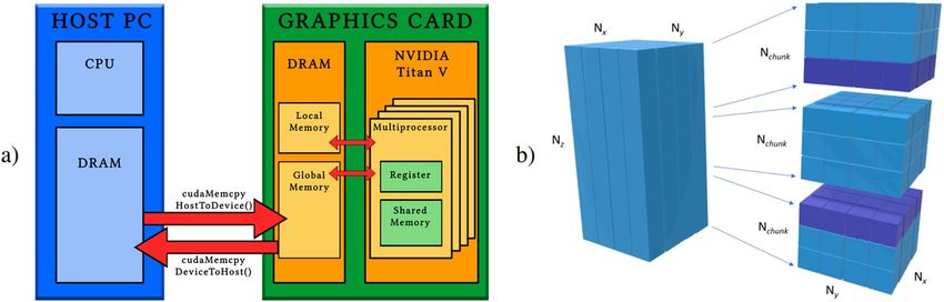
Figure 1(a) illustrates a draft of the tomosynthesis device for the specific case of the breast imaging: the X-ray
source emits a cone beam at each angle and its trajectory is restricted from the classical circular one to a C-shape
path. In Fig. 1(b) we report a more technical draw of the DBT geometry mashed on the YZ-plane in order to
better visualize the device setting, and in Fig. 1(c) we show the X-ray cone beam projection for one recording unit
on the detector. Due to the lack of data, the resolution of the reconstructed images along the in-depth Z-direction
is coarser than in the XY-plane. Moreover, the incomplete data sampling leads to well-studied artifacts. In par-
ticular, DBT images present two different types of artifacts: in-plane artifacts, consisting in a dark path in the
direction of the source motion around the dense objects, and in-depth artifacts, appearing as Nθ shadows in the
slices preceding and following the object along the Z-direction24.
More specifically, the quality of the reconstructed images depends on the number Nθ of acquired projections,
typically from 10 to 25, and on the angular range, usually from 15 to 50 degrees.
Materials. We have tested the proposed SGP method on two real data sets, fitting the European DBT
Protocol22, obtained by the digital system Giotto Class of the IMS Giotto Spa company and on a synthetic data
set obtained by simulating the projections of a digital phantom with the Giotto geometry. In Giotto apparatus,
the reference system is set as in Fig. 1(b). In the central position, the X-ray source is approximately 69 cm above
the detector and it shoots Nθ = 11 projections with a low dose protocol, in a very limited angular range from
−15 to 15 degrees. The flat detector has 3580 × 2812 square recording units with edges equal to 0.085 mm and
it is large enough to contain the widest compressed breast projections. As usual habit, in order to speed up the
reconstruction phase, in a preprocessing step the projections are cut to eliminate those portions of the data which
do not contain useful information for the breast reconstruction. If the resulting crop consists of nx × ny pixels for
each projection, then the available data set has size Nd = nx × ny × Nθ. The system uses a polychromatic ray with
Scientific Reports | (2020) 10:43 | https://doi.org/10.1038/s41598-019-56920-y 2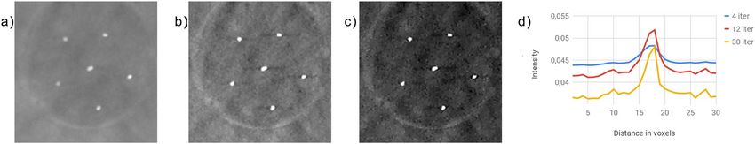
www.nature.com/scientificreports/                                                             www.nature.com/scientificreports

                          Figure 1. (a) Draft of the DBT system. (b) Picture of the DBT geometry mashed on the YZ plane. The breast is
                          constricted by compression paddles which are parallel to the breast supporting table and the detector plane (XY
                          plane). (c) A schematic draw of the projection process of the volume onto a single detector unit from a view in a
                          mashed 2D representation on the YZ plane. Scanning from the k − th position of the X-ray source, the yellow
                          cone of X-rays represents the projecting rays on the i − th pixel area (in blue). It intersects the object in the
                          magenta volume, hence all the voxels contributing to this projection are highlighted by bold edges. The
                          contribution of each voxel in the projection is proportional to the magenta portion inside the voxel itself.

                          energies in a narrow range around 20 keV to avoid the photon scattering. As often happens in CT reconstruction
                          algorithms, we approximate the polychromatic ray with a monochromatic one.
                              The first data set (D1) considered has size 3000 × 1500 × 11 and is obtained by scanning the Tomophan
                          Phantom TSP004, by The Phanto Laboratory25. The phantom contains aluminum Test Objects (TOs) embedded
                          into a clear urethane material and it has a semi-circular shape with a thickness of 42 mm. Due to its structure, this
                          Quality Control (QC) accreditation phantom is used for different tests (see the phantom data sheet25). Among
                          them, we concentrate on evaluating the homogeneity of the in-plane aluminum objects, the contrast between the
                          luminescent aluminum objects and the dark background, and the measure of the noise in the background. In
                          particular, in the reconstructed image we will focus on three 0.500 mm aluminum beads spaced 10 mm along the
                          Z-direction and hence positioned on three different layers.
                              The second data set tested (D2) has size 3000 × 1500 × 11 and it is obtained by scanning the BR3D Breast
                          Imaging Phantom26 (model 020), produced by the CIRS company, which is widely used to assess the detectability
                          of lesions of different sizes. The objects of interests, constituted by microcalcifications, fibers and masses, are
                          within a heterogeneous background composed by epoxy resin to simulate pure adipose and pure glandular tis-
                          sues, mixed together to mimic a real breast. In particular, we will analyze the reconstruction of a cluster of CaCO3
                          small beads, simulating microcalcifications of 0.290 mm in diameter.
                              Finally, we have tested the SGP algorithm on a simulated data set (D3), obtained from a digital phantom we
                          designed. The D3 data set has 3200 × 1100 × 11 elements, computed as projections of the digital phantom under
                          the geometric setting of the Giotto Class device onto a detector with 0.100 mm element pitch. We added Gaussian
                          noise with SNR = 50 to the computed projections (where the SNR value is computed as the logarithm of the ratio
                          between the noisy projections and the noise, multiplied by a factor of 20), to better simulate a real X-ray acqui-
                          sition. Our phantom reproduces the main features of the BR3D Breast Imaging Phantom: it contains several test
                          objects reproducing microcalcifications, fibers and masses, immersed into a uniform adipose-like background.
                          The attenuation coefficients of the test objects and background are taken from a reconstruction of the BR3D
                          Breast Imaging Phantom performed on a commercial system. The analysis on the reconstructed images carried
                          out in the next subsection will concentrate on the detection of a cluster containing 0.300 mm diameter beads,
                          simulating microcalcifications of medium size.
                              The data sets analysed during the current study are available at the website: https://cloud.hipert.unimore.it/s/
                          ptqjtMdwXA7sc5N.

                          Reconstructions.          In this paragraph we evaluate the quality of the reconstructions obtained with the pro-
                          posed SGP method on the data sets presented above. We are interested in monitoring how the algorithm performs
                          for an increasing number of iterations, hence we focus on the reconstructions achieved in 4, 12 and 30 iterations.
                              The volume to be reconstructed is discretized into Nv = Nx × Ny × Nz volumetric elements (voxels), where Nx,
                          Ny, Nz are the number of elements along the three Cartesian directions. We observe that in DBT imaging Nv > Nd.
                          The reconstructions of real phantoms have in-plane voxel size of 0.090 mm, whereas the in-depth one is 1.000
                          mm. In all the tests, the regularization parameter λ has been tuned by a trial and error procedure. The images pre-
                          sented in this section show slices of the reconstructed volume parallel to the XY-plane. We remind that the source
                          moves along the C-shaped path on the Y direction. For each phantom, the intensities of the reconstructions are
                          shown in the same gray scale (as arbitrary unit).

Scientific Reports |   (2020) 10:43 | https://doi.org/10.1038/s41598-019-56920-y                                                             3
www.nature.com/scientificreports/                                                               www.nature.com/scientificreports

                          Figure 2. (a–c) Crops of the reconstructions from data set D1, provided in 4, 12 and 30 iterations by the SGP
                          algorithm, respectively. They are represented in the same gray scale. The yellow rectangle is the uniform area for
                          the computation of the mean and standard deviation (StdDev) of the background. (d) The in-plane profile of
                          interest on the metal artifacts. (e) Comparison between the profiles of interest in (d) at different iterations. (f)
                          The in-plane profile of interest on the reconstructed aluminum bead. (g) Comparison between the profiles of
                          interest in (f) at different iterations. In (e,g) the blue, red and yellow line corresponds to the solution at 4, 12 and
                          30 iterations, respectively.

                          Figure 3. (a–c) Crops of the reconstructions from data set D2, provided by the SGP algorithm in 4, 12 and
                          30 iterations, respectively. They are represented in the same gray scale. (d) Comparison between the in-plane
                          profile of interest along the Y axis of the central bead at different iterations. The blue, red and yellow line
                          corresponds to the solution after 4, 12 and 30 iterations, respectively.

                          Tomophan phantom results. We report in Fig. 2 some results obtained on the D1 data set. Figure 2(a–c) show
                          the reconstructions after 4, 12, 30 iterations inside a region of 160 × 320 pixels (corresponding to 14.4 mm × 28.8
                          mm) on the layer 19, where the lower metallic sphere is on focus. The yellow rectangle in figures (a–c) defines
                          the region where we computed the mean and the standard deviation (StdDev) values reported under each corre-
                          sponding figure in order to analyze the background uniformity and the noise. Above the bead, we can also see the
                          expected metallic artifacts produced by the two specks located on layers 39 and 29. The artifacts corresponding
                          to the highest speck are in the form of 11 (i.e., the number of projections views) small circles, while the artifacts
                          produced by the central sphere are in the form of a light strip. The intensity of these artifacts can be analysed on
                          the profile identified by the orange line of Fig. 2(d); the reconstructions of the profile at different iterations are
                          compared in Fig. 2(e).
                              As concerns the in focus bead, we study the orange profile in Fig. 2(f) compared among the three considered
                          reconstructions in Fig. 2(g). The blue line shows that after 4 iterations the recovered values inside the sphere are
                          quite low and non-uniform, whereas the bead detection improves getting higher values of about 0.092 and 0.115
                          in the reconstructions at 12 and 30 iterations, respectively.

                          BR3D breast phantom results. Now we analyse the results obtained from the data set D2, characterized by
                          breast-like background and objects of interest. They are perfectly on focus on the selected layer. In Fig. 3(a–c) we
                          report the reconstruction crops corresponding to a 145 × 145 pixel region (13.05 mm × 13.05 mm) containing a
                          cluster of microcalcifications. In Fig. 3(d) we plot the corresponding in-plane profiles on the central speck along
                          the Y-direction.

Scientific Reports |   (2020) 10:43 | https://doi.org/10.1038/s41598-019-56920-y                                                                 4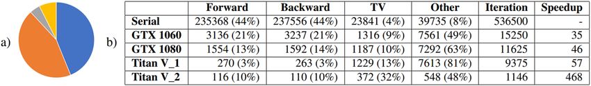
www.nature.com/scientificreports/                                                             www.nature.com/scientificreports

                          Figure 4. (a–c) Crops of the reconstructions from the simulated data set D3, provided by the SGP algorithm
                          in 4, 12 and 30 iterations, respectively. They are represented in the same gray scale. (d) Plot of the objective
                          function (1) versus the number of iterations. The red labeled dots report the values at 4, 12, 30 iterations and
                          at convergence. (e–g) Magnified views of the object inside by the yellow box for each reconstruction. (h) The
                          profile of interest along the Y-direction. (i) Comparison between the in-plane profiles at different iterations
                          and the ground truth. The green dotted profile shows the ground truth target, the blue, red and yellow line
                          corresponds to the reconstructed profile at 4, 12 and 30 iterations; the black dots show the profile obtained when
                          the convergence criterion is met.

                          Digital phantom results. In order to better analyse the accuracy of the MBIR approach in the challenging task
                          of a microcalcification detection, we present here the results obtained on the simulated D3 data set. The digital
                          phantom to be reconstructed from the D3 data set has size 3000 × 1000 × 50 with voxel size of 0.100 mm along
                          the X and Y axes and 1.000 mm along the Z direction. Figure 4(a–c) show the results obtained from D3 inside the
                          173 × 173 pixel ROI (corresponding to 17.3 mm × 17.3 mm) of the central layer of the synthetic phantom, con-
                          taining small microcalcifications. We have zoomed over one microcalcification in Fig. 4(e–g) where we can appre-
                          ciate how the 3-voxel wide object is already detected after only 4 iterations. Fig. 4(d) shows the behaviour of the
                          objective function minimized in (1) with respect to the iteration number. In Fig. 4(i) we plotted the profile of the
                          yellow line of Fig. 4(h) reconstructed after 4, 12 and 30 iterations and, with black dots, the solution obtained when
                          the convergence criterion is met (i.e., after 64 iterations). The green dotted line corresponds to the exact profile.

                          Parallel executions. The reconstructing software has been implemented in C code on a commercially avail-
                          able high end computer, equipped with Intel i7 7700K CPU at 4.2 GHz, 32 GB of RAM and 1 TB of Solid State
                          Disk (SSD), and its parallel implementation has been performed on NVIDIA GPUs by means of the CUDA
                          SDK27. The program has been tested on different GPUs, with different memories, number of CUDA cores and,
                          obviously, price point.
                             In details, we have considered the following GPU boards:

                          •   GTX 1060: 6 GB of RAM, 1280 CUDA cores, launch price 250$;
                          •   GTX 1080: 8 GB of RAM, 2560 CUDA cores, launch price 700$;
                          •   Titan V: 12 GB of RAM, 5120 CUDA cores, launch price 3000$.

                              We tested two different parallel implementations on the Titan V board: the first one (denoted as Titan V_1)
                          has the same approach considered for the GTX 1060 and GTX 1080 boards, where the data cannot be fully stored
                          in RAM and many data transfers between the CPU and the GPU are required during each SGP iteration, while
                          the second (denoted as Titan V_2) exploits the larger GPU RAM to store all the needed data. For more details on
                          the parallel implementations, please refer to the corresponding section.
                              The results shown in this paragraph are obtained on the D3 synthetic data set, whose volume is made of
                          Nv = 1.5·108 voxels. We have identified four main tasks in the SGP algorithm: the Forward and Backward projec-
                          tions, the TV evaluation and all the remaining operations (Other), mainly consisting of scalar products and vector
                          sums. We will analyse the parallel algorithm performance through these four tasks.
                              By profiling a serial execution of the program, we can draw the pie chart in Fig. 5(a) of the computational
                          time for the different tasks composing a single SGP iteration (for a comprehensive description of the algorithm,
                          please see the Methods sections): 88% of the time is spent for the Forward and Backward projections, 4% for the
                          evaluation of the TV function and of its gradient and 8% for all remaining SGP operations.
                              Figure 5(b) shows the execution times in milliseconds per iteration for each of the 4 computational kernels;
                          the last column reports the global speedup. The time required for a Forward or Backward projection decreases
                          from about 4 minutes in the serial execution to 1–3 seconds on the GTX boards and to less than 300 milliseconds

Scientific Reports |   (2020) 10:43 | https://doi.org/10.1038/s41598-019-56920-y                                                             5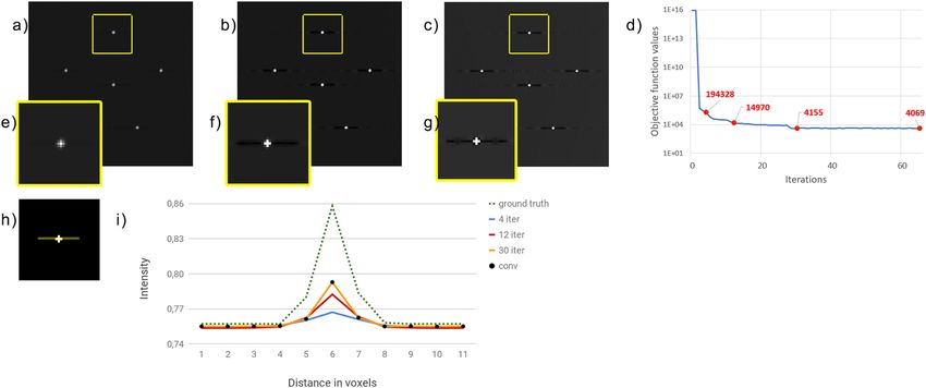
www.nature.com/scientificreports/                                                              www.nature.com/scientificreports

                          Figure 5. Computational time of a single SGP iteration (a) Pie chart of time spent for the four considered
                          kernels: Forward projection in blue, Backward projection in orange, TV evaluation in gray and all remaining
                          computations in yellow. (b) The table reports in each row the computational time of the four considered kernels
                          and, in brackets, their percentage with respect to the whole iteration time (column 6); the resulting speedup is
                          reported in column 7. All the times are in milliseconds.

                          Figure 6. Results for an increasing number of projection angles. (a) Computational time as a function of the
                          number of projection angles for the different boards. GTX 1060 is represented with an orange line (diamonds),
                          GTX 1080 with a yellow line (dots) and TitanV_1 with a green line (squares). (b) Table containing in each row
                          the information corresponding to a data set with Nθ projection angles: in columns 2 and 3 number of elements
                          and of nonzeros entries of the projection matrix A; in columns 4, 5 and 6 computational times in milliseconds.

                          for the Titan V_1 case. The parallelization of the TV function reduces the time from 23 seconds to 1 second, while
                          the execution time for Other decreases from about 40 to 7 seconds: these times are almost constant on all the three
                          boards since they are mainly due to data communications between CPU and GPU, which is independent from
                          the considered GPU board. Different performances are provided by the Titan V_2 case which achieves a speedup
                          of almost 470. We remark that the reported times correspond to an SGP iteration with only one execution of the
                          inner backtracking loop; each further backtracking step requires to evaluate only the TV component of the objec-
                          tive function, but it does not involve Forward or Backward projections.
                              Figure 6 shows the time per iteration on the three considered GPUs for data sets simulated by projecting the
                          digital phantom used in D3 with a varying number of angles Nθ ∈ {11, 21, 31, 41}.

                          Discussion
                          Looking at Fig. 2 and recalling the characterizations of the Tomophan Phantom, we can make the following
                          remarks. It is evident from Fig. 2(a–c) that for increasing iterations the contrast between the lower aluminum
                          sphere and the background enhances. Moreover, when the algorithm approaches the solution of (1), the sphere
                          gets more and more homogeneous inside, as can be viewed by the plots in Fig. 2(g). The mean and standard devi-
                          ation reported under Fig. 2(a–c) confirm that the noise keeps very low along the iterations. This proves that the
                          TV regularization term efficiently smooths the noise and that a suitable value for the regularization parameter has
                          been chosen. There are visible artifacts in the upper part of the images which are due to the small number of pro-
                          jection angles. However, from the plots in Fig. 2(e) we observe that their amplitude is very small and their contrast
                          from the background decreases with ongoing iterations. We also notice that all the artifacts are spread along the
                          Y axis direction according to the X-ray source motion. From all the above considerations, we can conclude that
                          increasing the iterations from 4 through 30 improves the quality of the reconstructed image for this test phantom.
                              The images in Fig. 3(a–c) show how the small beads of the microcalcification cluster are detected by the
                          solver after very few iterations, but with low contrast from the background. After 30 iterations, the contrast is far
                          enhanced. Figure 3(d) provides a double piece of information on solution changes during the iterations: it con-
                          firms that the contrast improves with the increasing number of iterations and that the microcalcification width
                          gets closer to the expected one of 290 micrometers (corresponding to about 3 voxels wide).
                              By analysing the results of the D3 data set we compare the reconstructed images with a ground truth. The reg-
                          ularizing effect of the TV prior is visible in Fig. 4(e–g), where the object spread is progressively reduced in favour
                          of a higher contrast with the background. Figure 4(i) confirms that values obtained for the microcalcification get
                          closer to the ground truth by increasing the number of iterations, whereas the exact background is recreated from
                          the first iterations. Since the black dots, representing the solution when the convergence criterion is met, overlap
                          the 30 iteration profile, we can conclude that the reconstruction after 30 iterations is the best possible to obtain.
                          We can also point out that the plot in Fig. 4(d) shows a remarkable decrease of the objective function in the first
                          iterations. As expected, there is a discrepancy between the computed solution and the exact one which is mainly
                          due to the sub-sampling of data in the DBT acquisition process.
                              From the performed tests we can conclude that the proposed model-based method, considering the L2-TV
                          mathematical model and using the SGP optimization algorithm, provides accurate DBT image reconstructions
                          in few tens of iterations. Concerning the comparison with other iterative optimization algorithms, the SGP algo-
                          rithm exploits a scaling acceleration strategy for improving the performance of the standard Gradient Projection

Scientific Reports |   (2020) 10:43 | https://doi.org/10.1038/s41598-019-56920-y                                                              6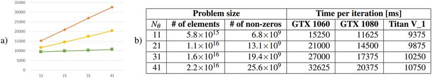
www.nature.com/scientificreports/ www.nature.com/scientificreports
Barzilai-Borwein (GPBB) method14 and the GPBB method has been proved to outperform widely used alternat-
ing minimization methods in the work by Park et al.9.
As we stated in the Introduction, the drawback of model-based methods is the long computational time
required. From the results presented in Fig. 5 we can notice that the computational times are dramatically reduced
in the parallel algorithm execution, with speedups ranging from 35× to 57× thanks to increasing computational
power for GTX1060, GTX1080 and Titan V boards. The execution of the Titan V_2 version further breaks down
the time, getting a speedup of almost 500, due to the particular implementation that avoids most of the data
transfer between the CPU and the GPU memory. Figure 6 proves that our parallel implementation linearly scales
with the size of the problem, providing different slopes for the different boards. In particular the Titan V_1 has
an incremental slope of 50 with respect to the GTX 1060 which is about 600, showing an enhanced scalability.
We can state that the proposed parallel implementation drastically cuts down the computational time, making
the execution times for the reconstruction of real volumes compatible with clinical requirements. This is possible
thanks to the ability of the SGP algorithm to provide suitable reconstructions in a few tens of iterations, which
can be performed in less than one minute by the most recent boards, like the Titan V. Taking into account that
the market of GPUs rapidly evolves towards more and more powerful and less costly boards, the proposed MBIR
approach represents a useful tool for achieving the goal of getting large volumetric images of superior quality at
affordable costs in the near future.
Methods
Scaled gradient projection method. In this paragraph we briefly describe the serial version of the SGP
algorithm which has been implemented to solve the minimization problem (1) for DBT reconstruction. The SGP
method is a first-order descent method for the solution of a general minimization problem of the form:
n
arg minx≥0f (x ), where x ∈ and f : n → is a convex differentiable function. In order to accelerate the clas-
sical Gradient Projection method, SGP introduces at each iteration k a scaling procedure18, by multiplying the
descent direction −∇f (x(k)) by a diagonal matrix Dk with entries in the interval 1 , ρk , ρk > 1, (we call Dρ the set
ρk k
of these matrices). Moreover, SGP exploits Barzilai-Borwein28 type rules for the choice of the steplength to ensure
a fast decrease of the objective function.
In details, after initializing x(0) ≥ 0, γ , σ ∈ (0, 1), 0 < α min ≤ α max , α 0 ∈ [α min , α max ], ρ0 > 0, D0 ∈ Dρ ,
0
the following steps are repeated for k = 0, 1… until a stopping criterion is satisfied.
1. Compute the scaled descent projected direction d(k) as d (k) = P+(x(k) − αkDk∇f (x(k))) − x(k), where P+(z)
is the Euclidean projection of the vector z ∈ n onto the non negative orthant.
2. Perform a backtracking on the computed direction d(k) starting with η = 1:
while f (x(k) + ηd (k)) > f (x(k)) + ση∇f (x(k))T d (k)
η = γ η;
3. Compute the new iterate: x(k+1) = x(k) + ηd (k).
4. Update ρk+1 = 1 + 1015 /(k + 1)2.1 and the diagonal scaling matrix Dk+1 ∈ Dρ .
k +1
5. Update the steplength αk+1 ∈ [α min , α max ].
The update of the scaling matrix Dk+1 is performed through a splitting of the gradient of the objective function
in its positive and negative parts as in14 and the definition of ρk+1 is aimed at avoiding restrictive bounds on the
diagonal entries of Dk+1 in the initial phase of the iterative process and satisfying the SGP convergence condi-
tions19 by asymptotically forcing Dk+1 towards the identity matrix. The update of the steplength αk+1 is obtained
by using an alternate Barzilai-Borwein strategy; in particular, we use adaptive alternations of the two classical
Barzilai-Borwein rules proposed in29 and applied also in14.
The algorithm is stopped when:
f (x(k)) − f (x(k−1)) < 10−6 f (x(k)) or k > maxiter (2)
where maxiter is the maximum number of iterations allowed. For more implementation details and for the con-
vergence properties of SGP refer to18,19. Even if the theoretical convergence rate O(1/k) on the objective function
values is lower than the rate O(1/k 2) of some optimal first-order methods17,30, the practical performance of SGP
method is very well comparable with the convergence rate of the optimal algorithms19.
Discrete mathematical model. The MBIR methods for CT image reconstruction are built on the discreti-
zation of the Lambert-Beer law, relating the acquired and emitted intensities of X-rays31 in the tomographic pro-
cess. The resulting model is a linear system of the form Ax = b where b collects all the Nd = Nθ × nx × ny
tomographic noisy projections, acquired during Nθ X-ray scans as nx × ny projection images, lexicographically
reordered into a vector shape; the unknown x is a Nv-dimensional vector resulting from the 3D discretization of
the volume. The operator projecting a volume x onto the detector according to the geometry of the CT device is
called Forward Projection (FwP). This is mathematically modeled by computing an Nd × Nv coefficient matrix A,
where each element represents the geometrical contribution of one voxel to one pixel of the detector for each
projection angle, and multiplying the matrix by a Nv-dimensional vector of the object space. The operator acting
from the projection space to the object space is called Backward Projection (BwP) and it is implemented via mul-
tiplication of AT by a Nd-dimensional vector of the projection space.
Scientific Reports | (2020) 10:43 | https://doi.org/10.1038/s41598-019-56920-y 7www.nature.com/scientificreports/ www.nature.com/scientificreports
Figure 7. (a) Logical view of a system composed by host and accelerator. The data which are stored in the host
memory (DRAM) must be transferred to the graphics card memory (Global Memory) to perform the
computations and subsequently the results must be transferred back to be saved in DRAM. (b) Schematic draw
of the partitioning into chunks of a volume. The data (on the left) are divided into Nz /Nchunk chunks. Each chunk
is sent and processed independently in the SGP parallel kernels. Only in the execution of the kernel computing
the TV function and its gradient, the purple slices of adjacent blocks are added to each chunk for the
computation of the finite differences on the border elements.
In the particular case of DBT, due to the sub-sampling of the limited angle geometry, Nd < Nv , hence the linear
system Ax = b is under-determined and admits infinite solutions. In order to force the uniqueness of the solution
and enhance the quality of the reconstruction, the problem is formulated as a minimization task as in (1), where
the objective function is defined as:
Nv
1 1
f (x ) = LS(x ) + λTV (x ) = Ax − b22 + λ ∑ ∇xj22 + β 2 .
2 2 j=1 (3)
Here, ∇xj2 is computed with respect to the three Cartesian directions with forward differences, while β > 0 is a
small constant introduced to overcome the non-differentiability of the discrete TV function whenever ∇xj2 is
zero for some j.
The function f(x) defined in (3) represents the objective function of the constrained minimization problem
that we solve with the SGP method, whose gradient is: ∇f (x ) = AT Ax − AT b + λ∇TV (x ). We remark that in,
the serial execution, the main computational cost at each SGP iteration is given by one FwP and one BwP involv-
ing the matrix-vector product by A and AT in the gradient formula (as shown in Fig. 5(a)). Moreover, the matrix
is too large to be stored in central memory and it must be re-evaluated at each matrix-vector operation (further
details in “Parallel implementation”). The computation of the matrix A plays a key role in the accuracy of the CT
modeling. Among the several approaches available in literature to define the tomographic matrix, we considered
the distance-driven (DD) one, proposed for the 3D geometry in 200432: it fits very well the CBCT geometry and is
suitable to be split among many processors. The draft in Fig. 1(c) schematically represents the DD Forward
Projection process for one pixel i, in a 2D scheme of the coronal view. In particular, fixed an angle θk and a pixel i,
the corresponding row of A contains the weights representing the contribution of all the voxels to the projection
onto the pixel i. To compute the weights, the DD algorithm first identifies which voxels are crossed by the X-rays
reaching the i − th pixel (the voxels with bold edges in Fig. 1(c)); then it quantifies the contribution of all and only
the identified voxels as the volume of the intersection between each voxel and the X-ray beam. We observe that A
is a very sparse matrix; in our tests, it always has a density factor of the order of 10−7. To compute the ∇TV (x )
function in each voxel, we used forward differences involving the voxel values14.
Parallel implementation. The proposed SGP method is suitable for parallel implementation on GPU as
reported in33,34. We describe in this section the parallel implementation of the SGP method for DBT image recon-
struction. We exploit the massive parallel architecture of the GPUs by distributing the work to hundreds of small
cores. A high level of parallelism is achieved by exploiting hundreds of computing pipelines, usually grouped into
processing clusters, which can work both in single and double precision. Within each of these processing clusters,
one hardware scheduler dispatches small groups of threads to the pipelines. To manage the communications
between the CPU and the GPU, the division of the work and the partition of thread in blocks, we use CUDA27, a
well-known Application Programming Interface developed by NVIDIA.
As already observed, the typical size of the data is so large that storing the whole matrix A in RAM is unfea-
sible. For example, in the data set D3 this would amount to (3000 × 1000 × 50) × (3200 × 1100 × 11) = 5.8·1015
elements (about 46 Petabytes in double precision data), which is much larger than the capacity of the most recent
RAM. Furthermore, the number of non-zero elements (see Fig. 6(b)) makes the storage of A in a sparse matrix
data structure inconvenient, since it would involve too large data transfer from the CPU memory to the GPU
one, representing a crucial bottleneck for the GPU performance (see Fig. 7(a)). In D3 data set, a sparse matrix
data structure representation requires at least 110 GB and the considered GPUs take about ten seconds for the
Scientific Reports | (2020) 10:43 | https://doi.org/10.1038/s41598-019-56920-y 8www.nature.com/scientificreports/ www.nature.com/scientificreports
memory transfer (almost an order of magnitude more than our approach). As a consequence, we organize the
parallelization of the FwP and BwP operations by computing the non-zero entries of A every time we need them.
Fixed Nthread as the number of threads per block, we created a grid of⌈Nv /Nthread⌉ blocks. Within this configu-
ration, each thread i independently computes the i − th row of the system matrix A according to the DD
strategy.
In the FwP evaluation, each thread i computes the product between the i − th line of A and the column vector
and saves the result in the i − th position of the resulting vector. Due to the independence of all these computa-
tions, we do not need any data access synchronization. Inside the BwP step we call exactly the same DD function
to compute the matrix A, hence we perform the product involving AT in a vector manner. Each thread i still com-
putes one row of A (i.e., column of AT ), it multiplies the contribution of each j − th voxel to the i − th element of
input vector and atomically sums the result to the j − th element of output vector.
For the parallelization of the TV and its gradient, we only need to operate on the values of the voxels. However,
the data access pattern is not coalesced and this limits the speedup of its implementation. All remaining computa-
tions in the SGP steps (previously labelled by Other) are vector operations and they are mainly executed in parallel
with CUBLAS library functions provided within the CUDA environment.
All the computations are performed in double precision arithmetic, since the results obtained with single
precision numbers were not satisfying. As a result, we need more than 11 GB of GPU memory to process the D3
data set. Since not all the commercial GPUs are equipped with such a large amount of memory, each parallel task
in the Fwp, BwP, TV and Others is separately executed on the GPU on portions of data (called chunks) and the
final results are collected on the CPU memory. Hence, the vectors of size Nv or Nd involved in the parallel compu-
tations are divided into chunks of size Nx × Ny × Nchunk and nx × ny × nchunk, respectively, where both Nchunk and
nchunk are integers depending on the memory available on the device. An example is depicted in Fig. 7(b). Since
the amount of data transferred between the CPU and the GPU is constant, the number of chunks does not have a
significant impact on overall performance.
Received: 3 April 2019; Accepted: 13 December 2019;
Published: xx xx xxxx
References
1. Males, M., Mileta, D. & Grgic, M. Digital breast tomosynthesis: A technological review. In Proceedings ELMAR-2011, 41–45 (IEEE,
2011).
2. Andersson, I. et al. Breast tomosynthesis and digital mammography: a comparison of breast cancer visibility and birads classification
in a population of cancers with subtle mammographic findings. European radiology 18, 2817–2825 (2008).
3. Das, M., Gifford, H. C., O’Connor, J. M. & Glick, S. J. Penalized maximum likelihood reconstruction for improved microcalcification
detection in breast tomosynthesis. IEEE Transactions on Medical Imaging 30, 904–914 (2010).
4. Feldkamp, L. A., Davis, L. & Kress, J. W. Practical cone-beam algorithm. Josa a 1, 612–619 (1984).
5. Beister, M., Kolditz, D. & Kalender, W. A. Iterative reconstruction methods in x-ray ct. Physica medica 28, 94–108 (2012).
6. Sidky, E. Y. et al. Enhanced imaging of microcalcifications in digital breast tomosynthesis through improved image-reconstruction
algorithms. Medical physics 36, 4920–4932 (2009).
7. Sidky, E. Y., Jørgensen, J. H. & Pan, X. Convex optimization problem prototyping for image reconstruction in computed tomography
with the chambolle–pock algorithm. Physics in Medicine & Biology 57, 3065 (2012).
8. Sidky, E. Y., Kao, C.-M. & Pan, X. Accurate image reconstruction from few-views and limited-angle data in divergent-beam ct.
Journal of X-ray Science and Technology 14, 119–139 (2006).
9. Park, J. C. et al. Fast compressed sensing-based cbct reconstruction using barzilai-borwein formulation for application to on-line
igrt. Medical physics 39, 1207–1217 (2012).
10. Jia, X., Lou, Y., Li, R., Song, W. Y. & Jiang, S. B. Gpu-based fast cone beam ct reconstruction from undersampled and noisy projection
data via total variation. Medical physics 37, 1757–1760 (2010).
11. Matenine, D., Goussard, Y. & Després, P. Gpu-accelerated regularized iterative reconstruction for few-view cone beam ct. Medical
physics 42, 1505–1517 (2015).
12. Sidky, E. Y. & Pan, X. Image reconstruction in circular cone-beam computed tomography by constrained, total-variation
minimization. Physics in Medicine & Biology 53, 4777 (2008).
13. Loli Piccolomini, E. & Morotti, E. A fast total variation-based iterative algorithm for digital breast tomosynthesis image
reconstruction. Journal of Algorithms & Computational Technology 10, 277–289 (2016).
14. Loli Piccolomini, E., Coli, V., Morotti, E. & Zanni, L. Reconstruction of 3d x-ray ct images from reduced sampling by a scaled
gradient projection algorithm. Computational Optimization and Applications 71, 171–191 (2018).
15. McGaffin, M. G. & Fessler, J. A. Alternating dual updates algorithm for x-ray ct reconstruction on the gpu. IEEE Transactions on
computational imaging 1, 186–199 (2015).
16. Graff, C. G. & Sidky, E. Y. Compressive sensing in medical imaging. Applied optics 54, C23–C44 (2015).
17. Jensen, T. L., Jørgensen, J. H., Hansen, P. C. & Jensen, S. H. Implementation of an optimal first-order method for strongly convex
total variation regularization. BIT Numerical Mathematics 52, 329–356 (2012).
18. Bonettini, S., Zanella, R. & Zanni, L. A scaled gradient projection method for constrained image deblurring. Inverse Problems 25,
015002 (2008).
19. Bonettini, S. & Prato, M. New convergence results for the scaled gradient projection method. Inverse Problems 31, 095008 (2015).
20. Coli, V. L., Ruggiero, V. & Zanni, L. Scaled first-order methods for a class of large-scale constrained least square problems. In AIP
Conference Proceedings, vol. 1776, 040002 (AIP Publishing, 2016).
21. Flores, L. A., Vidal, V., Mayo, P., Rodenas, F. & Verdú, G. Parallel ct image reconstruction based on gpus. Radiation Physics and
Chemistry 95, 247–250 (2014).
22. European Reference Organisation for Quality Assured Breast Screening and Diagnostic Services. www.euref.org. Protocol for the
Quality Control of the Physical and Technical Aspects of Digital Breast Tomosynthesis Systems.
23. Bernardi, D. et al. Digital breast tomosynthesis (dbt): recommendations from the italian college of breast radiologists (icbr) by the
italian society of medical radiology (sirm) and the italian group for mammography screening (gisma). Radiol. Med. 122, 723–730
(2017).
24. Hu, Y.-H., Zhao, B. & Zhao, W. Image artifacts in digital breast tomosynthesis: Investigation of the effects of system geometry and
reconstruction parameters using a linear system approach. Medical physics 35, 5242–5252 (2008).
Scientific Reports | (2020) 10:43 | https://doi.org/10.1038/s41598-019-56920-y 9www.nature.com/scientificreports/ www.nature.com/scientificreports
25. Tomophan Image Quality Phantom. https://www.phantomlab.com/tomophan-phantom. Tomophan Phantom - The Phantom
Laboratory.
26. Computerized Imaging Reference Systems. https://www.cirsinc.com/products/a11/51/br3d-breast-imaging-phantom/. BR3D Breast
Imaging Phantom, Model 020.
27. Nvidia. Cuda programming guide version 10.0. Nvidia Corporation (2018).
28. Barzilai, J. & Borwein, J. M. Two-point step size gradient methods. IMA journal of numerical analysis 8, 141–148 (1988).
29. Frassoldati, G., Zanni, L. & Zanghirati, G. New adaptive stepsize selections in gradient methods. Journal of Industrial and
Management Optimization 4, 299–312 (2008).
30. Nesterov, Y. Introductory lectures on convex optimization (Kluwer Academic, Dordrecht, 2004).
31. Epstein, C. Introduction to the mathematics of medical imaging (SIAM, Philadelphia, 2007).
32. De Man, B. & Basu, S. Distance-driven projection and backprojection in three dimensions. Physics in Medicine & Biology 49, 2463
(2004).
33. Zanella, R. et al. Towards real-time image deconvolution: application to confocal and sted microscopy. Scientific reports 3, 2523
(2013).
34. Ruggiero, V., Serafini, T., Zanella, R. & Zanni, L. Iterative regularization algorithms for constrained image deblurring on graphics
processors. Journal of Global Optimization 48, 145–157 (2010).
Acknowledgements
The authors thank the anonymous reviewers for their valuable comments and suggestions. This research has been
partially supported by GNCS-INDAM Italy (Research Projects 2018).
Author contributions
E.M. and E.L.P., designed the experiments, R.C., J.C.H., E.M. and L.Z., designed the algorithm and executed the
experiments, R.C., E.L.P., E.M. and L.Z. analysed the results and wrote the paper. All the authors reviewed and
approved the manuscript.
Competing interests
The authors declare no competing interests.
Additional information
Correspondence and requests for materials should be addressed to E.L.P.
Reprints and permissions information is available at www.nature.com/reprints.
Publisher’s note Springer Nature remains neutral with regard to jurisdictional claims in published maps and
institutional affiliations.
Open Access This article is licensed under a Creative Commons Attribution 4.0 International
License, which permits use, sharing, adaptation, distribution and reproduction in any medium or
format, as long as you give appropriate credit to the original author(s) and the source, provide a link to the Cre-
ative Commons license, and indicate if changes were made. The images or other third party material in this
article are included in the article’s Creative Commons license, unless indicated otherwise in a credit line to the
material. If material is not included in the article’s Creative Commons license and your intended use is not per-
mitted by statutory regulation or exceeds the permitted use, you will need to obtain permission directly from the
copyright holder. To view a copy of this license, visit http://creativecommons.org/licenses/by/4.0/.
© The Author(s) 2020
Scientific Reports | (2020) 10:43 | https://doi.org/10.1038/s41598-019-56920-y 10You can also read