Estimation of Basin scale turbulence distribution in the North Pacific Ocean using CTD attached thermistor measurements
←
→
Page content transcription
If your browser does not render page correctly, please read the page content below
www.nature.com/scientificreports
OPEN Estimation of Basin‑scale
turbulence distribution in the North
Pacific Ocean using CTD‑attached
thermistor measurements
Yasutaka Goto1,4*, Ichiro Yasuda1, Maki Nagasawa1, Shinya Kouketsu2 & Toshiya Nakano3,5
A recently developed technique for microstructure measurement based on a fast-response thermistor
mounted on a conductivity-temperature-depth equipment was used on eight cruises to obtain 438
profiles. Thus, the spatial distribution of turbulent dissipation rates across the North Pacific sea
floor was illustrated, and was found out to be related to results obtained using tide-induced energy
dissipation and density stratification. The observed turbulence distribution was then compared
with the dissipation rate based on a high-resolution numerical ocean model with tidal forcing, and
discrepancies and similarities between the observed and modelled distributions were described. The
turbulence intensity from observation showed that the numerical model was overestimated, and
could be refined by comparing it with the observed basin-scale dissipation rate. This new method
makes turbulence observations much easier and wider, significantly improving our knowledge
regarding ocean mixing.
Ocean turbulence with a vertical diffusivity of O (10–4 m2 s−1) is1 required to maintain the vertical water-mass
distribution in the deep North Pacific. Therefore, quantifying the vertical diffusivity is important to evaluate
the meridional overturning circulation and water-mass distribution. A recent modelling s tudy2 reproduced an
observed Δ14C distribution in the deep Pacific using a spatially variable vertical diffusivity distribution, which
was constructed on the basis of high-resolution models3 for internal gravity waves generated by tides. However,
model-based vertical diffusivity has not yet been sufficiently validated via direct microstructure observations
owing to their scarcity.
Basin-scale turbulence distributions have been demonstrated4,5 using an indirect method that is based on the
fine-scale parameterizations6–10 of the interior ocean, far from turbulence generation sites (surface and bottom
boundary layers, areas close to rough topographies and coastal boundaries, and strong current regions) using
fine-scale O (10–100 m) density and velocity observations along World Ocean Circulation Experiment-hydro-
graphic sections. Additionally, global horizontal distribution and seasonal variability have been demonstrated
using fine-scale density measurements with profiling fl oats11,12, and energy dissipation rate estimations from
fine- and micro-scale observations have also been compiled13. These studies have revealed that turbulent energy
dissipation rates increase over rough bottom topographies, and their spatial variability is related to internal wave
energy fields.
While studies based on fine-scale parameterizations have revealed considerable information on turbulence
in the deep ocean, the applications of parameterizations are limited to regions where the Garrett–Munk (GM)
wave field14 is undistorted. Although studies in which distortion was taken into consideration have also been
conducted10, direct microstructure measurement is still needed to precisely estimate turbulence intensity. How-
ever, direct microstructure measurements have been performed only in specific regions, such as ridges and straits,
as was the case in the Brazil basin15, Hawaiian R idge16, Izu-Ogasawara R idge17, and Kuril S trait18,19. Therefore,
basin-scale observations using direct microstructure measurements are necessary.
1
Atmosphere and Ocean Research Institute, The University of Tokyo, Kashiwanoha 5‑1‑5, Kashiwa,
Chiba 277‑8564, Japan. 2Research Institute for Global Change, Japan Agency for Marine-Earth Science
and Technology, Natsushima 2‑15, Yokosuka, Kanagawa 237‑0061, Japan. 3Japan Meteorological Agency,
Otemachi 1‑3‑4, Chiyoda, Tokyo 100‑8122, Japan. 4Present address: Kushiro Local Meteorological Office, Japan
Meteorological Agency, Saiwai‑cho 10‑3, Kushiro, Hokkaido 085‑8586, Japan. 5Present address: Nagasaki Local
Meteorological Office, Japan Meteorological Agency, Minamiyamate‑machi 11‑51, Nagasaki, Nagasaki 850‑0931,
Japan. *email: gotoyasutaka@met.kishou.go.jp
Scientific Reports | (2021) 11:969 | https://doi.org/10.1038/s41598-020-80029-2 1
Vol.:(0123456789)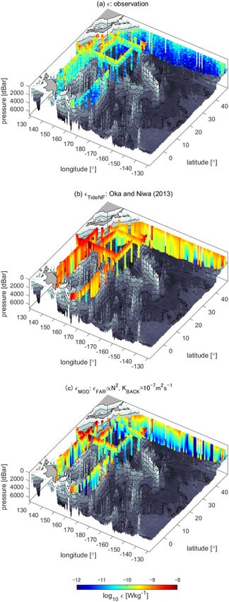
www.nature.com/scientificreports/
Figure 1. Station locations for 438 CTD-attached fast-response thermistor measurements. The stars denote the
full-depth stations, with casts all the way down to the sea floor, and the circles represent the other casts, which
extended down to a depth of 2000 m. Stations corresponding to KS16-06 with magenta colour are under KS16-
08 (green) and KS16-09 (yellow), and are masked. See Table S1 for cruise codes.
In this study, direct microstructure measurements are demonstrated along eight large-scale hydrographic
sections in the North Pacific via the application of the new platform for microstructure observations, which uses
conductivity-temperature-depth (CTD) attached thermistors. This system20–22 can be used to efficiently evaluate
the turbulent energy dissipation rate (ε) in the range of 1 0–11–10–8 W kg−1 with data quality controls considering
the effects of the movement of the CTD-frame as well as data adjustment on the attenuation of the temperature
gradient spectra. The observation-based turbulence intensity can then be compared with the tide-induced baro-
clinic energy and the density stratification as well as the energy dissipation rate based on the fine-scale param-
eterization. Furthermore, it can be quantitatively compared with the dissipation obtained based on the ocean
general circulation model (OGCM) so as to clarify the discrepancy between the model and the observations.
Results
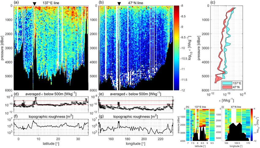
Turbulence distribution in the North Pacific. Two basin-scale, vertical cross-sections of ε from fast-
response thermistor measurements along 137°E and 47°N (Fig. 1 for station locations) are shown in Fig. 2a,b,
respectively, with the vertical profiles of ε averaged in each section (Fig. 2c). The overall features of ε were as
follows: (1) vertically, ε was found to be generally large at depths from the surface to the pycnocline. (2) The
137°E-mean ε at each depth was three times that in 47°N (Fig. 2a–c). (3) Relatively large ε values were observed
over rough bottom topographies, such as the Ngulu Atoll at 8°N 137°E, the Emperor Seamount at 47°N 170°E,
and the slope edge at 47°N 50°W. Quantitatively, ε averaged from a depth of 500 m to the bottom (Fig. 2d–e) cor-
responded to the topographic roughness represented by the variance of the bottom depth (Fig. 2f–g). These fea-
tures obtained using the present CTD-attached method are similar to those reported in previous s tudies4,5,11–13.
Further analysis of feature (1) showed that the observed ε correlated well with the strength of stratification
(Fig. 3a), i.e. the squared buoyancy frequency, N2 (s−2) (= gα(∂T/∂z + γ) − gβ∂s/∂z, where g represents the gravita-
tional acceleration (m s−2), T represents temperature (°C), s represents salinity (psu), α represents the coefficient
of thermal expansion (°C−1), β represents the coefficient of saline contraction (psu−1), and γ represents the adi-
abatic lapse scale (°C m−1), with the high correlation coefficient, r = 0.74 (see Table S2 in the “Supplementary
Information” for statistical data).
For features (2) and (3), the horizontal distribution of the depth-integrated observed dissipation, ∫ρεdz,
depended on the energy distribution of the internal waves driven by tidal forcing (Fig. 3b). Depth-integrated
observed energy dissipation, ∫ρεdz, from the full-depth casts was found to be correlated (r = 0.58) with the
model-based horizontal energy distribution of the internal wave generation Ec(x,y) (see “Methods”). It was also
found to be correlated (r = 0.66) with the horizontal distribution of the model-based energy dissipation, Ed(x,y),
estimated using tide-forced internal waves. These relationships indicate that the depth-integrated observed
dissipation, ∫ρεdz, is regulated by the energy distribution of the tide-induced internal waves. The relationship
between the observed ε and topographic roughness was explained by the tide-generating internal wave energy
distribution. The higher internal wave activity along 137°E seemed to induce a relatively higher ε averaged over
the sections than along 47°N (Fig. 2c).
Scientific Reports | (2021) 11:969 | https://doi.org/10.1038/s41598-020-80029-2 2
Vol:.(1234567890)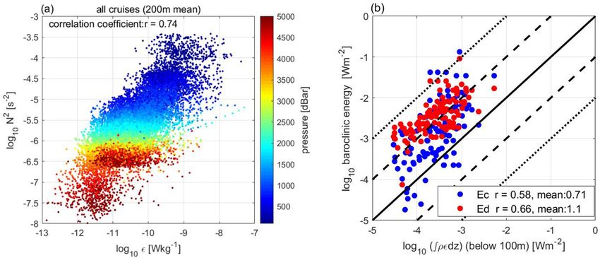
www.nature.com/scientificreports/
Figure 2. Vertical cross-sections of turbulent energy dissipation rate, ε. Along (a) 137°E (RF16-06) and (b)
47°N (MR-14-04) with triangular marks corresponding to areas close to the Ngulu Atoll and the Emperor
Seamount. In (a) and (b), ε is averaged over 50 m after eliminating the data at Wsd > 0.2 W–0.06 and Wmin. (c)
Vertical profile of horizontally averaged ε for each section. (d,e) Vertically averaged ε below 500 m to exclude
surface dissipation, where the red lines denote values at ε = 10–10 and 10–9 W kg−1. (f,g) Topographic roughness
at each station, defined as the variance of bathymetric height (m2) obtained from ship depth s oundings23,
calculated in 60 km square regions. (h,i) Enlarged views of the Ngulu Atoll and the Emperor Seamount.
Figure 3. Relationship between ε and N2 and baroclinic tide energy. (a) Relationship between the observed
energy dissipation, ε, and the squared buoyancy frequency, N2. Colours denote pressure. (b) Relationship
between depth-integrated observed energy dissipation, ∫ρεdz, and model-based depth-integrated baroclinic
energy conversion rate, Ec (blue dots), representing the generation of internal waves by tidal forcing, and
the relationship between ∫ρεdz and depth-integrated tide-induced energy dissipation, Ed (red dots), both
correspond to MR-14-04 and RF16-06. X-axis: depth-integrated ρε from a 100-m depth to the bottom,
excluding the surface 100-m layer to avoid the influence of wind. Y-axis: Ec and Ed are estimated in the m odel2
based on the 3-D tide-driven m odel3. Ec and Ed simulated with the resolution (1/15°) model are multiplied by
1.5 as in the model2. “r” in the legend represents the correlation coefficient in logarithmic scale and “mean” is the
average of log(Y/X).
Scientific Reports | (2021) 11:969 | https://doi.org/10.1038/s41598-020-80029-2 3
Vol.:(0123456789)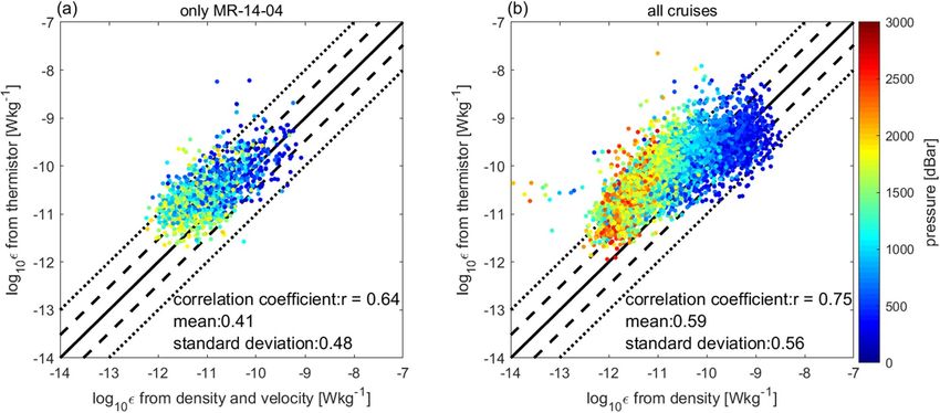
www.nature.com/scientificreports/
Figure 4. Comparison of ε with fine-scale parameterizations. (a) ε based on fine-scale velocity and density
using Lowered Acoustic Doppler Current Profilers (LADCP) and CTD10. (b) ε based on only fine-scale density8.
Data are averaged in 320-m segments. The surface data that included the upper 100-m layer are not used. In (a),
data with pressure > 2000 dbar are excluded because the accuracy of the measurement of LADCP is low in the
deep ocean. In (b), data with N2 < 10–6 s−2 are excluded since the estimation of the vertical gradient of density is
difficult in the low stratified regions. “mean” and “standard deviation” in the legend represent the average and
the standard deviation of log(Y/X), respectively.
Close to the sea floor, ε values were not high. However, bottom-intensified mixing has been demonstrated in
previous studies24. One possible reason for the low ε values could be the lack of data corresponding to the area
close to the sea floor. Since the frame falls slowly within 100 m above the sea floor, most data were eliminated by
the data rejection criterion of Wsd > 0.2W–0.06 (see “Methods”); thus, the data became sparse. These findings can
be attributed to the absence of the bottom-intensified dissipation structure, which was modelled as maximum
dissipation at the bottom and decayed exponentially with h eight25. Further analysis of the data quality and the
improvement of the analysis method are required to quantify the turbulence, 100 m above the sea floor. Another
possible reason is that roughness is not sufficient to generate strong turbulence in many stations along 137°E and
47°N, except in areas with very rough topography, such as the Ngulu Atoll and the Emperor Seamount (Fig. 2h,i).
Comparison with fine‑scale parameterizations. Most data were obtained in the interior ocean, where
fine-scale parameterizations6–10 are applicable. Consistency between the present method and the previous fine-
scale parameterization method can support the validity of the new CTD-attached thermistor method. Along
the 47°N section, where velocity data are available, we calculated εFINE using a new m ethod10 based on fine-
scale velocity and density profiles, while considering the spectral distortion depending on the ratio of fine-scale
kinetic to potential energy (Rω). The calculated εFINE values were found to be correlated with the ε values obtained
using the CTD-attached method (r = 0.64), and the average of log(ε/εFINE) was within a factor of three (Fig. 4).
For the data corresponding to other sections, even the method involving the use of only density data8 resulted in
high correlation (r = 0.75), without the abnormal overestimation of ε.
Comparison with ε‑field used in ocean circulation model. The observed ε distribution was com-
pared with εTideNF (see “Methods”) used in the ocean circulation model2, which reproduced the Δ14C distribution
in the deep Pacific (TideNF model). The vertical εTideNF distribution close to the tide generation sites, εNEAR,
was assumed to exponentially decay above the sea floor with a decaying scale, h (= 500 m), and the vertically
integrated dissipation at each location was set to the local dissipation rate, q (= 1/3), of the baroclinic energy
conversion rate Ec(x,y) from the barotropic tides. Parameters h and q were based on previous observational and
numerical studies24,25 and Ec(x,y)3. The vertical εTideNF distribution far away from the tide generation sites, εFAR,
was assumed to be vertically uniform2 for simplicity. The background εTideNF distribution, εBACK, was assumed
to have the vertically uniform diffusivity2, KBACK (= 10–5 m2 s−1). Please refer to the “Methods” section for the
details on εTideNF.
Notably, εTideNF was much higher (over ten times) than the observed ε (Fig. 5), while the correlation coefficient
between them for depths below 500 m based on data from eight cruises was r = 0.55, suggesting that spatial vari-
ability has some similarity with the observations. The relatively high εNEAR over the rough topographies (such
as the Ngulu Atoll at 8°N 137°E, the Emperor Seamount at 47°N 170°E, and the slope edge at 47°N 50°W) were
estimated in the model; it was observed that they contributed to the representation of the observational features
of the spatial changes in ε (Figs. 2a,b and 5a,e). Considering that the constant background diffusivity was used
in the model, it was observed that εBACK (= KρN2Γ−1 = 10−5N2 × 0.2–1) depends on the strength of stratification,
Scientific Reports | (2021) 11:969 | https://doi.org/10.1038/s41598-020-80029-2 4
Vol:.(1234567890)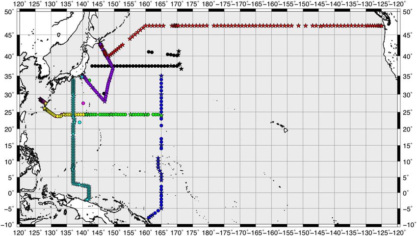
www.nature.com/scientificreports/
Figure 5. εTideNF along 137°E (left) and 47°N (right). (a,e) Near-field, εNEAR, (b,f) Far-field, εFAR, (c,g)
Background, εBACK, (d,h) εTideNF = εNEAR + εFAR + εBACK. The squared buoyancy frequency is observation-based, and
the mixing efficiency, Γ, is 0.2.
N2. Thus, εBACK contributed to the representation of the dependency of stratification (Figs. 2a,b and 5c,g), which
was also detected in ε (the correlation coefficient between log(ε) and log(N2) was 0.74; Fig. 3a). Further, εFAR,
which was assumed to be vertically uniform in the model2, showed the greatest deviation from the observed
ε, and had an order of magnitude that was larger than that of the observed ε, even far from the rough bottom
topography (Figs. 2a,b and 5b,f).
odel2, while the near-field diffusivity was set following the parameterization25 and considering the
In the m
observations24, the background and far-field diffusivity were not based on direct observations, but were set so
Scientific Reports | (2021) 11:969 | https://doi.org/10.1038/s41598-020-80029-2 5
Vol.:(0123456789)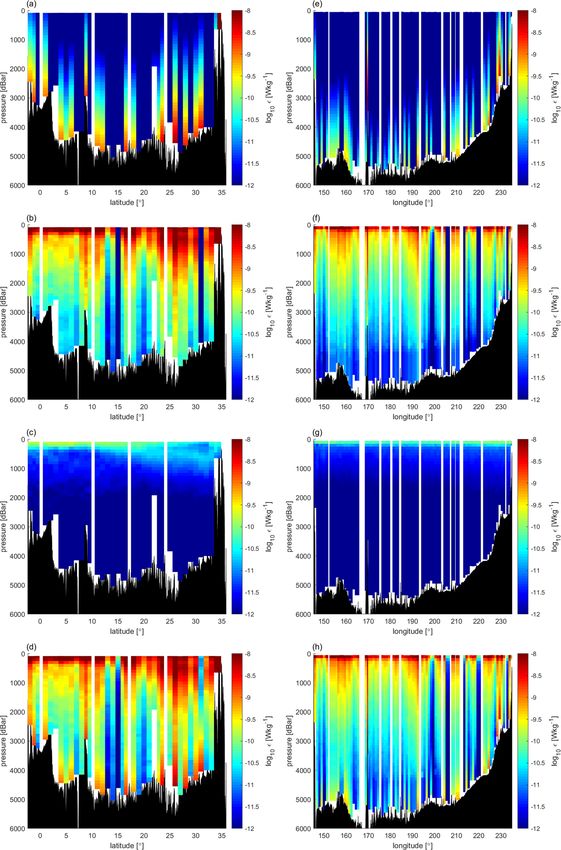
www.nature.com/scientificreports/
Figure 6. Occurrence of diapycnal diffusivity Kρ (= 0.2ε/N2). The vertical axis denotes the data quantity. Data
averaged at 200 m after data screening are displayed.
that the predicted tracer field follows the observations. Thus, we introduced another parameterization to modify
εTideNF, referred to as εMOD. The vertical structure, FFAR(z), of εFAR (Eq. 2 in “Methods”) was modified to be propor-
tional to the squared buoyancy frequency, N2, as FFAR(z)= (N 2 /N2 )H−1, where the overbar denotes the vertical
mean and H represents the sea floor depth26. This form is consistent with the observational fact that ε is corre-
lated with N2 (Fig. 3a). Background diffusivity was then changed to KBACK = 10–7 m2 s−1 given that the minimum
value of the observations was 1 0–7 m2 s−1 (Fig. 6). After revision, εMOD became closer to the observed ε within a
factor of three and with a relatively high correlation coefficient (Fig. 7; r = 0.50 between Fig. 8a,c), whereas large
discrepancies were observed between εTideNF and the observed ε (Fig. 8a,b). In the revised εMOD, εFAR was found to
be the main contributor to the major part of the ocean, except at depths close to the sea floor, where εNEAR showed
dominance, with εBACK being very small (Fig. 7b,f). This modification implies that the baroclinic energy gener-
ated at the bottom propagates more widely with the longer damping time scale compared to the TideNF model.
Discussion
There were uncertainties in both the observation- and model-based estimates. One reason for these uncertainties
was the variable response time of the FP07 thermistors. In this study, to capture micro-scale turbulence, all tem-
perature gradient spectra were corrected and multiplied by the double-pole low-pass filter function [1 + (2πfτ)2]2
with the time constant, τ = 3 ms, to compensate for the attenuation of the frequency spectra owing to the insuf-
ficient response speed. The time constants of the individual FP07 sensors could be varied between 1.9 and 5.6 ms
for the double-pole functions at 1/4 attenuation (“Methods”). Another uncertainty arose in the estimation of ε
in the weak turbulence range of ε < 10–10 W kg−1. This is because such weak turbulence could not be evaluated
based on micro-scale shear observations, which were used for the validation of the FP07 observations20. Thus,
ε in this range varied between 0 and 1 0–10 W kg−1.
The uncertainties associated with the response time and weak turbulence range were evaluated by compar-
ing the geometric means of the ratios of ε (Table 1), which could be varied by changing τ and/or ε in the range
ε < 10–10 W kg−1. When τ was changed, and keeping ε < 10–10 W kg−1, i.e. εBACK (the middle column), the ratio
varied from 0.398 to 1.49, and the uncertainty factor was approximately four. In contrast, when the background
ε was changed and τ was kept constant (τ = 1.9), and the uncertainty factor was approximately eight (the ratio
varied between 0.398 and 3.13). Even though all the differences among these cases were within a factor of ten
these results support the importance of time constant estimates for each probe as well as precise measurements
of weak turbulence below 1 0–10 W kg−1 in deep ocean.
It was also necessary to consider the temporal variability in turbulence intensity. The observation at each
station in this regard was performed only once. Actually, temporal variability with semi-diurnal and diurnal
tidal cycles exists. For example, in strong turbulence regions such as the Kuril Strait, the temporal variability
was larger than two orders of magnitude, and was related to the tidal c ycle18. It was expected that the distribu-
tion of ε in our observations will likely vary if the observations were made at the same stations. Thus, to obtain
representative ε values in such strong turbulence regions, further observations should be performed to estimate
the temporal average.
Scientific Reports | (2021) 11:969 | https://doi.org/10.1038/s41598-020-80029-2 6
Vol:.(1234567890)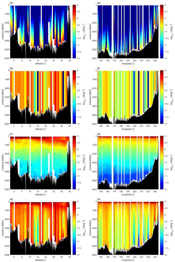
www.nature.com/scientificreports/
Figure 7. Modified εMOD distribution adjusted to the observed ε. (a,e) Near-field εNEAR, (b,f) Far-field εFAR, (c,g)
Background εBACK, (d,h) εMOD = εNEAR + εFAR + εBACK.
The local dissipation ratio, q (= 1/3), of the generated internal tide energy, Ec(x,y), and decay scale, h (= 500 m),
in near-field εNEAR have been proposed in previous numerical and observational s tudies24,25. The decay scale,
h, may not be constant, but might depend on the amplitude of tidal flow and the horizontal wavenumber of
the bottom t opography27. The data corresponding to this study were insufficient to determine h because a large
portion of the CTD casts could only descend to a depth of approximately 2000 m, failing to reach the sea floor.
Furthermore, the dissipation rate ε, from most of the full-depth casts decreased toward the bottom and did not
exhibit the exponential decay structure from the bottom. The bottom-enhanced structure was observed only in
the Ngulu Atoll at 8°N 137°E and the Emperor Seamount at 47°N 170°E, both of which are strong internal tide
generation sites with high baroclinic energy conversion from barotropic tides. To consider the spatial differences
Scientific Reports | (2021) 11:969 | https://doi.org/10.1038/s41598-020-80029-2 7
Vol.:(0123456789)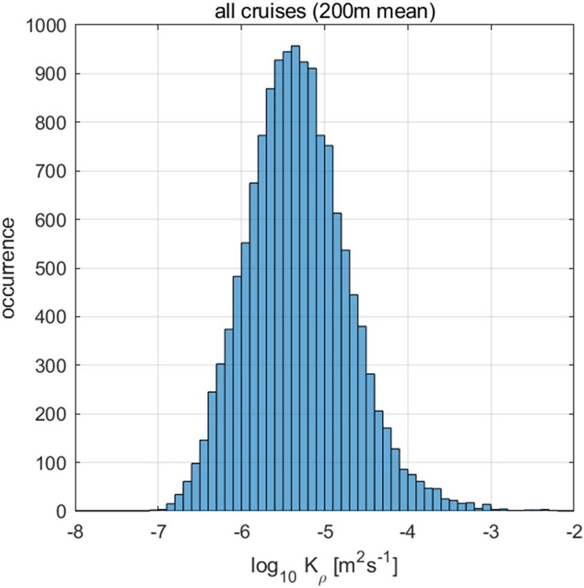
www.nature.com/scientificreports/
Figure 8. Comparison of 3-D ε distributions. Comparison of ε (a) Based on the CTD-attached thermistor
GCM2, which reproduced the radio-carbon isotope ratio in the Pacific, and (c)
observations, (b) based on the O
based on the modified model, within which the far-field ε is proportional to the squared buoyancy frequency,
N2, and the background value of ε is based on the observed minimum diapycnal diffusivity, Kρ = 10–7m2 s−1, to
make the model distribution closer to the observations.
Scientific Reports | (2021) 11:969 | https://doi.org/10.1038/s41598-020-80029-2 8
Vol:.(1234567890)www.nature.com/scientificreports/
ε < 10–10 W kg−1 is unchanged (original) ε < 10–10 W kg−1 is εBACK (minimum) ε < 10–10 W kg−1 is 10–10 (maximum)
τ = 1.9 (ms) 0.742 (0.738–0.745) 0.398 (0.392–0.404) 3.13 (3.06–3.19)
τ = 3.0 (ms) 1 0.572 (0.563–0.582) 3.70 (3.63–3.77)
τ = 5.6 (ms) 2.23 (2.21–2.25) 1.49 (1.46–1.53) 6.18 (6.10–6.26)
Table 1. Uncertainties in ε based on observations. The geometric means of the ratios between the modified
ε (changing τ and ε in ε < 10–10 W kg−1) and the original ε (the case of the middle row, the left column), with
95% confidence intervals of the bootstrap method are in the parentheses. The 200 m-mean data set of the ε
values corresponding to all observation points of the eight cruises were used. The three values correspond to
the uncertainty of the individual thermistors whose time constant based on spectrum double-pole correction
ranges between 1.9 and 5.6 ms. Another source of uncertainty is the weak turbulence region, ε < 10–10 W kg−1,
where ε is set to the background value (the middle columns), εBACK, or fixed at 10–10 (the right column). εBACK is
based on the observed minimum diapycnal diffusivity, i.e. εBACK = Kρ·N2·Γ−1 = 10–7·N2·0.2–1.
in h, it was necessary to accumulate bottom-reaching ε data. Additionally, in this study, parameter q was also
constant; possibly dependent on the latitude because diurnal internal waves cannot propagate at high latitudes
with a possibility of local dissipation intensifying28,29. To consider the latitudinal dependence of q, meridional
observations at the sea floor covering high latitudes are required.
For far-field dissipation, εFAR, the vertical structure proportional to N2 in εMOD was more suitable for the
reproduction of the observational distribution than the simple vertically uniform εFAR in εTideNF. This depend-
ency on N2 is consistent with the theory6, where ε ∝ N2E2 (E represents the fine-scale energy density) in the GM
internal wave field14. Additionally, the theory6 served as the basis for the existing fine-scale parameterizations7–10.
However, further research is required to explain how this N2-dependence is established from tide-induced
internal wave fields.
It is worth noting that the model-based energy dissipation Ed(x,y), and baroclinic energy conversion Ec(x,y),
were much greater than the depth-integrated observed ∫ρεdz regardless of the high correlation coefficients. Ec
100 m
(Ed) was 5 (13) times greater than bottom ρεdz (Fig. 3b). This magnitude of difference has also been reported
between directly measured ε and model-based forcing and dissipation estimates13, suggesting that dissipation
takes place in locations other than the observed sites, or close to the bottom or the surface, where the present
observations did not fully cover. However, this will be a subject of future studies owing to the uncertainties in
both the observations and models.
The background diffusion obtained in m odel 2 and those obtained in other modelling s tudies 29,30
KBACK = 10–5 m2 s−1, were two orders of magnitude larger than the minimum value obtained in this study, and
the total background energy dissipation accounted for more than 20% of the total dissipation in the upper
1000 m. KBACK was reduced to the observed minimum in this study. KBACK could increase if the dissipation by
the near-inertial internal waves forced by winds31 or internal lee waves due to current-topography interactions32
were included in εBACK. Although the dissipation related to N2 was included in a component of the tide-generated
dissipation εFAR, which constituted a major part of the internal tide-induced energy dissipation in this study, it
might have been appropriate to include it in εBACK if the wind and internal lee waves have a large contribution
to the dissipation related to N2.
In this study, direct microstructure observations were conducted in the deep North Pacific using fast-response
thermistors attached to CTD frames. After careful data quality control, through which data resulting from the
movement of the frames was eliminated, the basin-scale distribution of turbulence energy dissipation rate ε,
was revealed. High ε values were observed over the rough topography close to seamounts and ridges, where
reportedly, internal tides are generated. The ε values from the micro-temperature were found to be comparable
with that of the previous fine-scale parameterization estimation in the interior ocean within a factor of three.
Additionally, they also showed correlation with the internal tide energy dissipation and the squared buoyancy
frequency, N2. However, these ε values were 1/10 times smaller than those obtained using the previous OGCM,
which reproduced the deep Pacific water-masses fields. To adjust εTideNF to the observed ε, we proposed another
parameterization. By adjusting the vertical structure that is far from the internal tide generation sites (far-field) to
be proportional to N2, and by reducing the background constant diapycnal diffusivity to 10–7 m2 s−1, the difference
was modified to be within a factor of three. This indicates that widespread observations using the CTD-attached
thermistors with higher spatial and temporal resolutions can contribute to a more realistic representation of
diapycnal diffusivity distribution in OGCMs in the near future.
Methods
Observational data. A total of 438 vertical profiles of micro-temperature data were obtained during the
cruises of the R/V Keifu Maru, R/V Ryofu Maru, R/V Mirai, and R/V Hakuho Maru vessels in the North Pacific
(see Table S1 in the “Supplementary Information”). Full-depth observation of the sea floor was performed at all
the stations along the 47°N and 137°E sections. In the other sections, measurements were performed at several
stations down to a depth of 2000 m, with some being full-depth observations. For each location, a one-time
measurement was performed. The station locations are shown in Fig. 1.
The micro-temperature profilers, Micro Rider 6000 and AFP07, both manufactured by Rockland Scientific
Inc. (Canada), were installed on CTD frames of the cruises. Micro Rider 6000 was installed in the MR-14-04
cruise and AFP07 was installed in the remaining cruises. To avoid measurement of artificial turbulence caused
Scientific Reports | (2021) 11:969 | https://doi.org/10.1038/s41598-020-80029-2 9
Vol.:(0123456789)www.nature.com/scientificreports/
by the frames, the two fast-response thermistors (Fastip Probe model 07; henceforth FP07) were attached close
to the bottom of the frames (Fig. 1 of the s tudy21). Probes whose spectra fit the universal spectrum better was
used in this analysis.
Estimation of the energy dissipation rate, ε. Turbulent energy dissipation rates (ε) were estimated
using the relationship, ε = (2π)4kB4νκ2, where ν represents the kinematic viscosity (m2 s−1), κ represents the molecu-
lar thermal diffusivity (m2 s−1), and kB represents the Batchelor wavenumber of the temperature spectrum (cpm).
We estimated kB by fitting the universal spectrum to the observed temperature gradient s pectrum33,34. The data
processing was the same as in a previous s tudy21, based on the maximum likelihood estimation m ethod35. Each
spectrum was determined from a profile segment within 1 s and corrected using the double-pole low-pass filter
function36. Considering that each thermistor was not calibrated, the time constant, which represents the effect of
smoothing the microstructures due to relatively slow sensor response, was fixed at 3 ms20.
Time constant dependence of the sensor fall rates has been demonstrated in some previous s tudies36,37. The
faster the sensor fall rate, the smaller the time constant becomes; thus, the required correction is also smaller.
However, making corrections considering this characteristic could result in underestimation in areas with strong
turbulence21. When the sensor falls with a higher speed, higher frequencies are necessary to determine the
Kraichnan spectrum. These higher frequencies could be significantly attenuated, making it difficult to attain
full correction, regardless of the use of double- or single-pole functions. Consequently, the smaller correction
associated with the higher speed results in underestimation. Accordingly, the dependence of the time constant
on the sensor speed was not considered in this study.
To estimate kB, we only used the spectrum in the lower frequency domain avoiding using the high frequencies
dominated by electrical noise, which was determined by comparing the noise spectrum obtained with dummy
probes in our laboratory. The form of the fitted universal spectrum was the one34 with the fixed universal constant,
qK = 5.2638,39. After the fitting, automatic rejection criteria40 based on the shape of the observed spectrum were
applied on each spectrum to eliminate poorly fitted data.
Data screening. Given that the CTD-attached fast-response thermistor is a new platform for the measure-
ment of turbulence, a specific method for quality control was necessary. At times, not-free-fall measurements
generate artificial turbulence due to the CTD-frame or probes themselves, causing the overestimation of ε as
discussed in a previous study21. Such overestimation is frequently observed under the small descending rate
[W (ms−1)] and/or the large standard deviation of W [Wsd (ms−1)], when data from the R/V Hakuho Maru and
R/V Shinsei Maru are used. By eliminating the data satisfying Wsd > 0.2W − 0.06, the CTD-attached thermistor
could estimate the energy and thermal dissipation rate in a manner comparable to that of a free-fall thermistor21.
However, conditions generating artificial turbulence depend on the mode of operation, which might be dif-
ferent from one research vessel to another22. Data from the three other ships, the R/V Ryofu Maru, R/V Keifu
Maru, and R/V Mirai, in addition to those from the R/V Hakuho Maru were used in this study. Therefore, it was
expected that the turbulence data quality would be maintained. Here, we updated the condition for the elimina-
tion of the outliers by re-examining the data from the R/V Ryofu Maru (Supplementary Fig. S1).
Before data screening (Fig. S1b), relatively large ε values (> 10–8 W kg−1) were observed in the entire depth
range at latitudes 2–3°N, 13°N, 17–19°N, and 24–30°N, corresponding to the large Wsd (Fig. S1a), which could
be caused by ship rolling or pitching due to large surface waves owing to rough sea states. These overestimated ε
values were efficiently removed by the rejection criteria, Wsd > 0.2 W − 0.0621 (Fig. S1c). However, large ε patches
remained at the intermediate-to-deep levels as well as in the casts with large Wsd.
When the vertical profiles of the ε values based on the CTD-attached method as well as the fall rate, W, and
Wsd were carefully examined, the spikes of the ε values were eliminated based on the rejection c riteria21,40 (the red
dots in Fig. S2). However, in areas with small W and Wsd values, unnaturally large ε values, above 10–8 (W kg−1)
remained. Reportedly, decelerating W can cause artificial turbulence with a higher downward momentum, and
such turbulence is considered to keep up with the sensors at around the local minimum of the fall rate Wmin
(also in Fig. 7 in the paper21). Overestimated data at Wmin were not necessarily removed by the rejection criterion
Wsd > 0.2W − 0.06 because Wsd can also be very small in some cases. By eliminating data at Wmin in addition to
that in the range Wsd > 0.2W − 0.06, almost all the spurious ε values were removed (Fig. 2d). These combined
rejection criteria of Wsd > 0.2W − 0.06 and Wmin were used in this study.
Dependence of ε on individual thermistors. Temperature spectra obtained from thermistors are atten-
uated at high frequencies; thus, they need to be corrected. The form of the correction functions were single- or
double-pole low-pass filters36,41 with the time constant, τ, which is different for individual probes of the same
type due to the differences in glass coatings42. Since ε varies as τ changes, it was necessary to consider the range
of τ within which the probe was not calibrated. In this subsection, the uncertainty of τ was found to be between
1.9 and 5.6 ms in the double-pole low-pass filter function based on the following analysis. The ε from seven FP07
thermistors (εT) were compared with the ε values measured simultaneously using shear probes (εS). The free-fall
vertical microstructure profiler (VMP2000) manufactured by Rockland Scientific Inc. was employed in the four
cruises (Table S3). Data processing was based on the results of a previous s tudy20.
It is worth noting that εT is consistent with εS within a factor of three for all the thermistors examined in
this study. Although the dependence of the εT estimate on individual thermistors is evident as shown in Fig. S3,
some thermistors (serial number (S/N) 886, 1024, and 1025) showed that εT is larger than εS in the entire range
of 10–10 < εS < 10–7 W kg−1, whereas other thermistors (S/N 271 and 415) showed smaller values, even after all
the temperature gradient spectra were corrected using the same single-pole41 (SP: [1 + (2πfτ)2]) and double-
pole36 (DP: [1 + (2πfτ)2]2) correction functions with τ equal to 7 and 3 ms, respectively (Fig. S3a,b). This scatter
Scientific Reports | (2021) 11:969 | https://doi.org/10.1038/s41598-020-80029-2 10
Vol:.(1234567890)www.nature.com/scientificreports/
was likely caused by the time constant, τ, owing to differences in the glass coatings42. The degree of the scatter
depends on turbulence intensity, εS, and the difference between the probes was a factor of three at a relatively
strong turbulence intensity, εS, of approximately 1 0–7.5 W kg−1, while it was within a factor of two at a relatively
weak turbulence intensity, εS, of approximately 1 0–9.5 W kg−1. The dependence of the scatter on the turbulence
intensity, εS, could be attributed to the shift in the spectra to a higher frequency range, where attenuation is more
considerable.
We estimated the time constant, τ, for individual thermistors by modifying εT to εS (Fig. S3c,d). The optimal τ
range was between 3.0 and 10.2 ms for the SP and 1.9 and 5.6 ms for the DP functions. These values represent the
ranges of the τ uncertainty of the thermistors with unknown time constants and are consistent with the nominal
value of the time constant, 7 ± 3 ms for the SP function. Therefore, it was expected that the errors derived from
the uncertainty of the time constants would be at least 3.0–10.2 (ms) (SP) or 1.9–5.6 (ms) (DP). The uncertainties
of ε from the CTD-attached thermistors are discussed based on this result.
ε in the ocean general circulation model. The turbulent energy dissipation data used in the OGCM,
which were referred to as TideNF2, were compared with the observational data obtained in this study. The model
turbulent energy dissipation originally consisted of two types of horizontally 2-D (depth-integrated) data. First,
is the energy conversion rate from barotropic to baroclinic (internal) tides (Ec(x,y)), representing the local gen-
eration of internal tides, and second, is the local energy dissipation of the internal waves, (Ed(x,y)). Both datasets
were obtained from a 3-D high-resolution (1/15°) model forced by t ides3 and used after being multiplied by 1.5,
given that the global baroclinic conversion rate at the limit of zero grid spacing was approximately 1.5 times
larger than the grid spacing of 1/15°2. A 3-D distribution of energy dissipation rates εTideNF was constructed
using three components: (1) the near-field component, εNEAR, which represents the local dissipation close to
the generation site of the tide-generated internal waves over the rough topography, (2) the far-field component,
εFAR, which represents the dissipation of propagating internal waves away from the generation site, and (3) the
background component, εBACK, which represents the dissipation other than (1) and (2):
εTideNF = εNEAR + εFAR + εBACK . (1)
The dissipations of the three components were expressed as:
εNEAR = ENEAR x, y FNEAR (z)/ρ,
(2)
εFAR = EFAR x, y FFAR (z)/ρ, and
εBACK = KBACK N 2 / Ŵ,
where ρ represents the sea water density (kg m−3), N represents the buoyancy frequency (s−1), KBACK represents
the background diapycnal diffusivity, and Γ represents the mixing efficiency. KBACK = 10–5 m2 s−1 and Γ = 0.2 in the
TideNF model2. In this study, N was computed using the observed density data corresponding to each CTD cast.
F(z) represents the vertical structures of the near- and far-field components as in a previous s tudy2:
e−(H−z)/h
FNEAR (z) =
, and
h 1 − e−H/h (3)
FFAR (z) = 1/H,
where z is the depth (m), H is the bottom depth (m), and h is the decay scale from the bottom (m) of the near-
field dissipation. This exponential decay from the bottom topography of the near-field dissipation was based on
a previous modelling25 and observational study24. The far-field component was not based on the observations,
and for simplicity, it was assumed to be vertically uniform2.
The horizontally variables, ENEAR and EFAR represent the depth-integrated energy dissipation in the near- and
far-field, respectively. They were derived as follows:
ENEAR x, y = qEc(x, y) if qEc ≤ Ed,
(4)
ENEAR x, y = Ed(x, y) if qEc > Ed, and
EFAR x, y = Ed(x, y) − ENEAR x, y ,
where Ec represents the energy conversion rate from the barotropic tide to the baroclinic internal tide, Ed repre-
sents the depth-integrated energy dissipation in each water column (the sum of ENEAR and EFAR), and q represents
the ratio of local dissipation to the generated baroclinic energy (it was set to the constant value, q = 0.33)2,24.
Ec and Ed were calculated n umerically3 using 3-D Navier–Stokes equations under hydrostatic and Boussinesq
approximations as follows:
H
Ec(x, y) = gρ ′ ws dz, and
0
(5)
H
∂
′ ′
∂
′ ′
Ed(x, y) = Ec(x, y) − pu + pv dz,
∂x ∂y
0
Scientific Reports | (2021) 11:969 | https://doi.org/10.1038/s41598-020-80029-2 11
Vol.:(0123456789)www.nature.com/scientificreports/
where g represents acceleration due to gravity, ρ ′ represents the deviation of sea water density from the basic
field associated with the baroclinic tide motions, ws represents the vertical velocity resulting from the interaction
between the barotropic tidal flow and the bottom topography, and the overbar denotes the time average. u′, v′,
and p′ represent the eastward and northward velocities and the pressure perturbations associated with baroclinic
tidal motions, respectively.
In this study, the distribution of the energy dissipation rate was examined given that diapycnal diffusivity
depends on buoyancy frequency, mixing efficiency, and energy dissipation rate, and these three factors can be
different in the model and in the observations. Examples of the spatial distribution of εTideNF using the observed
buoyancy frequency field are shown in Fig. 5. εNEAR was large close to the rough bottom topography, which is
characterised by a large baroclinic energy. Farther from the bottom, εTideNF was dominated by εFAR and εBACK.
Additionally, εFAR was assumed to be vertically uniform, and it depends only on the horizontally variable dissi-
pation of remotely generated internal waves. εBACK was large in the upper ocean because it is proportional to N2.
Accordingly, εBACK accounted for more than 20% of all the dissipation rates in the upper 1000-m level.
Data availability
The datasets generated during this study are available in the following repository: https://ocg.aori.u-tokyo.ac.jp/
omix/GOTO_etal_SREP2020/. MATLAB was used in generating all the figures, except for Fig. 1.
Received: 7 June 2020; Accepted: 11 December 2020
References
1. Munk, W. H. Abyssal recipes. Deep Sea Res. Oceanogr. Abstr. 13(4), 707–730. https: //doi.org/10.1016/0011-7471(66)90602- 4 (1966).
2. Oka, A. & Niwa, Y. Pacific deep circulation and ventilation controlled by tidal mixing away from the sea bottom. Nat. Commun.
4, 2419. https://doi.org/10.1038/ncomms3419,Pubmed:24013486 (2013).
3. Niwa, Y. & Hibiya, T. Estimation of baroclinic tide energy available for deep ocean mixing based on three-dimensional global
numerical simulations. J. Oceanogr. 67(4), 493–502. https://doi.org/10.1007/s10872-011-0052-1 (2011).
4. Kunze, E., Firing, E., Hummon, J. M., Chereskin, T. K. & Thurnherr, A. M. Global abyssal mixing inferred from lowered ADCP
shear and CTD strain profiles. J. Phys. Oceanogr. 36(8), 1553–1576. https://doi.org/10.1175/JPO2926.1 (2006).
5. Kunze, E. Internal-wave-driven mixing: Global geography and budgets. J. Phys. Oceanogr. 47(6), 1325–1345. https://doi.
org/10.1175/JPO-D-16-0141.1 (2017).
6. Henyey, F. S., Wright, J. & Flatté, S. M. Energy and action flow through the internal wave field: An eikonal approach. J. Geophys.
Res. 91(C7), 8487–8495. https://doi.org/10.1029/JC091iC07p08487 (1986).
7. Gregg, M. C. Scaling turbulent dissipation in the thermocline. J. Geophys. Res. 94(C7), 9686–9698. https://doi.org/10.1029/JC094
iC07p09686 (1989).
8. Wijesekera, H. et al. The application of internal-wave dissipation models to a region of strong mixing. J. Phys. Oceanogr. 23(2),
269–286. https://doi.org/10.1175/1520-0485(1993)023%3c0269:TAOIWD%3e2.0.CO;2 (1993).
9. Polzin, K. L., Toole, J. M. & Schmitt, R. W. Finescale parameterizations of turbulent dissipation. J. Phys. Oceanogr. 25(3), 306–328.
https://doi.org/10.1175/1520-0485(1995)025%3c0306:FPOTD%3e2.0.CO;2 (1995).
10. Ijichi, T. & Hibiya, T. Frequency-based correction of finescale parameterization of turbulent dissipation in the deep ocean. J. Atmos.
Ocean. Technol. 32(8), 1526–1535. https://doi.org/10.1175/JTECH-D-15-0031.1 (2015).
11. Whalen, C. B., Talley, L. D. & MacKinnon, J. A. Spatial and temporal variability of global ocean mixing inferred from Argo profiles.
Geophys. Res. Lett. https://doi.org/10.1029/2012GL053196 (2012).
12. Whalen, C. B., MacKinnon, J. A., Talley, L. D. & Waterhouse, A. F. Estimating the mean diapycnal mixing using a finescale strain
parameterization. J. Phys. Oceanogr. 45(4), 1174–1188. https://doi.org/10.1175/JPO-D-14-0167.1 (2015).
13. Waterhouse, A. F. et al. Global patterns of diapycnal mixing from measurements of the turbulent dissipation rate. J. Phys. Oceanogr.
44(7), 1854–1872. https://doi.org/10.1175/JPO-D-13-0104.1 (2014).
14. Garrett, C. & Munk, W. Space-time scales of internal waves: A progress report. J. Geophys. Res. 80(3), 291–297. https://doi.
org/10.1029/JC080i003p00291 (1975).
15. Polzin, K. L., Toole, J. M., Ledwell, J. R. & Schmitt, R. W. Spatial variability of turbulent mixing in the abyssal ocean. Science
276(5309), 93–96. https://doi.org/10.1126/science.276.5309.93,Pubmed:9082993 (1997).
16. Klymak, J. M. et al. An estimate of tidal energy lost to turbulence at the Hawaiian Ridge. J. Phys. Oceanogr. 36(6), 1148–1164. https
://doi.org/10.1175/JPO2885.1 (2006).
17. Nagasawa, M., Hibiya, T., Yokota, K., Tanaka, Y. & Takagi, S. Microstructure measurements in the mid-depth waters of the North
Pacific. Geophys. Res. Lett. 34(5), L05608. https://doi.org/10.1029/2006GL028695 (2007).
18. Yagi, M. & Yasuda, I. Deep intense vertical mixing in the Bussol’Strait. Geophys. Res. Lett. https://doi.org/10.1029/2011GL050349
(2012).
19. Yagi, M. & Yasuda, I. A modified method for estimating vertical profiles of turbulent dissipation rate using density inversions in
the Kuril Straits. J. Oceanogr. 69(2), 203–214. https://doi.org/10.1007/s10872-012-0165-1 (2013).
20. Goto, Y., Yasuda, I. & Nagasawa, M. Turbulence estimation using fast-response thermistors attached to a free-fall vertical micro-
structure profiler. J. Atmos. Ocean. Technol. 33(10), 2065–2078. https://doi.org/10.1175/JTECH-D-15-0220.1 (2016).
21. Goto, Y., Yasuda, I. & Nagasawa, M. Comparison of turbulence intensity from CTD-attached and free-fall microstructure profilers.
J. Atmos. Ocean. Technol. 35(1), 147–162. https://doi.org/10.1175/JTECH-D-17-0069.1 (2018).
22. Yasuda, I. et al. Estimate of turbulent energy dissipation rate using free-fall and CTD-attached fast-response thermistors in weak
ocean turbulence. J. Oceanogr. https://doi.org/10.1007/s10872-020-00574-2 (2020).
23. Smith, W. H. F. & Sandwell, D. T. Global sea floor topography from satellite altimetry and ship depth soundings. Science 277(5334),
1956–1962. https://doi.org/10.1126/science.277.5334.1956 (1997).
24. St. Laurent, L. C., Toole, J. M. & Schmitt, R. W. Buoyancy forcing by turbulence above rough topography in the abyssal Brazil Basin.
J. Phys. Oceanogr. 31(12), 3476–3495. https://doi.org/10.1175/1520-0485(2001)031%3c3476:BFBTAR%3e2.0.CO;2 (2001).
25. St. Laurent, L. C., Simmons, H. L. & Jayne, S. R. Estimating tidally driven mixing in the deep ocean. Geophys. Res. Lett. 29(23),
21–21. https://doi.org/10.1029/2002GL015633 (2002).
26. Melet, A., Legg, S. & Hallberg, R. Climatic impacts of parameterized local and remote tidal mixing. J. Clim. 29(10), 3473–3500.
https://doi.org/10.1175/JCLI-D-15-0153.1 (2016).
27. Hibiya, T., Ijichi, T. & Robertson, R. The impacts of ocean bottom roughness and tidal flow amplitude on abyssal mixing. J. Geophys.
Res. Oceans 122(7), 5645–5651. https://doi.org/10.1002/2016JC012564 (2017).
Scientific Reports | (2021) 11:969 | https://doi.org/10.1038/s41598-020-80029-2 12
Vol:.(1234567890)www.nature.com/scientificreports/
28. Tanaka, Y., Hibiya, T., Niwa, Y. & Iwamae, N. Numerical study of K1 internal tides in the Kuril straits. J. Geophys. Res. 115(C9),
C09016. https://doi.org/10.1029/2009JC005903 (2010).
29. Tanaka, Y., Yasuda, I., Hasumi, H., Tatebe, H. & Osafune, S. Effects of the 18.6-yr modulation of tidal mixing on the North Pacific
bidecadal climate variability in a coupled climate model. J. Clim. 25(21), 7625–7642. https://doi.org/10.1175/JCLI-D-12-00051.1
(2012).
30. Hasumi, H., Yasuda, I., Tatebe, H. & Kimoto, M. Pacific bidecadal climate variability regulated by tidal mixing around the Kuril
Islands. Geophys. Res. Lett. https://doi.org/10.1029/2008GL034406 (2008).
31. D’Asaro, E. A. The energy flux from the wind to near-inertial motions in the surface mixed layer. J. Phys. Oceanogr. 15(8), 1043–
1059. https://doi.org/10.1175/1520-0485(1985)015%3c1043:TEFFTW%3e2.0.CO;2 (1985).
32. Nikurashin, M. & Ferrari, R. Global energy conversion rate from geostrophic flows into internal lee waves in the deep ocean.
Geophys. Res. Lett. https://doi.org/10.1029/2011GL046576 (2011).
33. Batchelor, G. K. Small-scale variation of convected quantities like temperature in turbulent fluid Part 1. General discussion and
the case of small conductivity. J. Fluid Mech. 5(1), 113–133. https://doi.org/10.1017/S002211205900009X (1959).
34. Kraichnan, R. H. Small-scale structure of a scalar field convected by turbulence. Phys. Fluids 11(5), 945–953. https://doi.
org/10.1063/1.1692063 (1968).
35. Ruddick, B., Anis, A. & Thompson, K. Maximum likelihood spectral fitting: The Batchelor spectrum. J. Atmos. Oceanic Technol.
17(11), 1541–1555. https://doi.org/10.1175/1520-0426(2000)017%3c1541:MLSFTB%3e2.0.CO;2 (2000).
36. Gregg, M. C. & Meagher, T. B. The dynamic response of glass rod thermistors. J. Geophys. Res. 85(C5), 2779–2786. https://doi.
org/10.1029/JC085iC05p02779 (1980).
37. Hill, K. D. Observations on the velocity scaling of thermistor dynamic response functions. Rev. Sci. Instrum. 58(7), 1235–1238.
https://doi.org/10.1063/1.1139444 (1987).
38. Bogucki, D., Domaradzki, J. A. & Yeung, P. K. Direct numerical simulations of passive scalars with Pr > 1 advected by turbulent
flow. J. Fluid Mech. 343, 111–130. https://doi.org/10.1017/S0022112097005727 (1997).
39. Bogucki, D. J., Luo, H. & Domaradzki, J. A. Experimental evidence of the Kraichnan scalar spectrum at high Reynolds numbers.
J. Phys. Oceanogr. 42(10), 1717–1728. https://doi.org/10.1175/JPO-D-11-0214.1 (2012).
40. Peterson, A. K. & Fer, I. Dissipation measurements using temperature microstructure from an underwater glider. Meth. Oceanogr.
10, 44–69. https://doi.org/10.1016/j.mio.2014.05.002 (2014).
41. Lueck, R. G., Hertzman, O. & Osborn, T. R. The spectral response of thermistors. Deep Sea Res. 24(10), 951–970. https://doi.
org/10.1016/0146-6291(77)90565-3 (1977).
42. Gregg, M. C. Uncertainties and limitations in measuring ε and χT. J. Atmos. Oceanic Technol. 16(11), 1483–1490. https://doi.
org/10.1175/1520-0426(1999)016%3c1483:UALIMA%3e2.0.CO;2 (1999).
Author contributions
Y.G. analysed the data and wrote the manuscript. I.Y. led the project and supervised the research. S.K. and T.N.
conducted the observations. M.N. initiated the CTD-attached FP07 analysis.
Competing interests
The authors declare no competing interests.
Additional information
Supplementary Information The online version contains supplementary material available at https://doi.
org/10.1038/s41598-020-80029-2.
Correspondence and requests for materials should be addressed to Y.G.
Reprints and permissions information is available at www.nature.com/reprints.
Publisher’s note Springer Nature remains neutral with regard to jurisdictional claims in published maps and
institutional affiliations.
Open Access This article is licensed under a Creative Commons Attribution 4.0 International
License, which permits use, sharing, adaptation, distribution and reproduction in any medium or
format, as long as you give appropriate credit to the original author(s) and the source, provide a link to the
Creative Commons licence, and indicate if changes were made. The images or other third party material in this
article are included in the article’s Creative Commons licence, unless indicated otherwise in a credit line to the
material. If material is not included in the article’s Creative Commons licence and your intended use is not
permitted by statutory regulation or exceeds the permitted use, you will need to obtain permission directly from
the copyright holder. To view a copy of this licence, visit http://creativecommons.org/licenses/by/4.0/.
© The Author(s) 2021
Scientific Reports | (2021) 11:969 | https://doi.org/10.1038/s41598-020-80029-2 13
Vol.:(0123456789)You can also read