Estimating the Demand for Railroad and Barge Movements of Corn in the Upper Mississippi River Valley

Estimating the Demand for
 Railroad and Barge Movements of Corn in the
 Upper Mississippi River Valley*
 January 2021

 by

 Tobias Sytsma and Wesley W. Wilson †

*This work was supported by Cooperative Agreement Number Agreement 18-TMTSD-TN-0012, with the Agricultural Marketing
Service (AMS) of the U.S. Department of Agriculture (USDA). The author gratefully acknowledges discussions with and
comments from Peter Caffarelli, Jesse Gastelle, Kelly Nelson, although any errors or omissions are those of the author.
Disclaimer: The opinions and conclusions expressed in this report do not necessarily represent the views of USDA or AMS.
†Sytsma, Rand Corporation (tobysytsma@gmail.com); and Wilson, Professor of Economics, University of Oregon
(wwilson@uoregon.edu).

 i

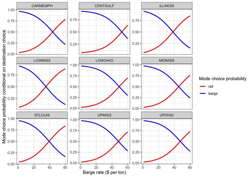
Table of Contents

Executive Summary................................................................................................................................... 1
1. Introduction ......................................................................................................................................... 5
2. Literature Summary ............................................................................................................................. 7
3. Modeling Shipper Decisions ................................................................................................................. 8
4. Data .................................................................................................................................................... 10
 4.1 Barge data .................................................................................................................................... 11
 4.2 Rail data........................................................................................................................................ 14
 4.3 Combined data ............................................................................................................................. 16
 4.4 Freight Rates ................................................................................................................................ 19
5. Results ................................................................................................................................................ 21
6. Summary and Conclusion ................................................................................................................... 27
References .............................................................................................................................................. 29
Appendix: Modeling Shipper Decisions ................................................................................................. 32

 ii

Executive Summary

Transportation is a key element in the movement of agricultural products to market. The level and nature

of demand for different modes has a significant influence on the prices agricultural shippers pay, the

routes that are taken, and whether public and/or private investments are warranted. Modal demands,

however, are influenced by the geography of the shippers and characteristics of the commodity

transported. Shippers located a long distance from the river tend to ship by rail (at least for long-haul

movements), while shippers located near the waterway typically ship by barge, as truck-to-barge rates

are often considerably lower than rail.

 The prices paid by shippers also depend on these same characteristics. While truck and barge

markets are often thought to be competitive, railroads have considerable latitude in the rates they charge,

and the range of observed prices is quite large. In areas where barge is a viable option, railroads may be

constrained by barge rates, while in areas where barge is not a feasible option, railroads may choose

higher prices (Anderson and Wilson (2008), Burton (1993), MacDonald (1987; 1989)). In between,

railroads can choose a set of prices that exclude rail to barge routings in favor of all-rail routings even

though the multimodal routing is less costly (Burton and Wilson (2006)).

 At the root of competition is the presence and availability of substitutes. As noted, in the case of

rail and barge transportation, barge is relatively more attractive for locations close to the river. However,

as the distance from the waterway increases, barge becomes less attractive and eventually is not used.

However, the catchment area for barge—the range at which barge is a feasible mode for shippers—has

received relatively little attention, and the relationship between modal demands and catchment areas

has typically not been investigated.

 These relationships are central not only to pricing but also to the feasibility of both public and

private infrastructure investments. For example, the U.S. Army Corps of Engineers (USACE) uses barge

demand models in their calculation of the benefits of waterway investments. Controversies over their

 1

planning models in the late 1990s led to a number of transportation demand studies intending to estimate

barge volumes for their calculations. 1 Most of these studies relied on survey data of shippers in a river

system (e.g., Columbia-Snake river valleys, Upper Mississippi-Illinois river valleys, and the Ohio). 2 From

the surveys, data were collected on shipper choices and options and analyzed using choice methods to

estimate demands. Generally, the spatial environment of shippers in these studies was reflected in the

choices made. That is, shippers located a long distance from the waterway typically chose rail, while

shippers near the waterway typically chose barge. In this sense, the spatial boundaries are inherent in

the choices made by the shippers and not used to define spatial boundaries (i.e., the catchment area for

barge). 3

 The overriding objective of this research is to accurately capture the linkages between the

demands for barge and rail freight movement. We develop a methodology—using data for corn, the top

agricultural product in terms of tonnage—that considers a wide range of catchment areas using non-

survey data. Essentially, we use available data within an area and estimate barge versus rail demand

choices. Our approach utilizes the unmasked confidential waybill sample (CWS) of the Surface

Transportation Board (STB) and the Waterborne Commerce Statistics (WCS) of the Army Corps of

Engineers. The former gives the origin and destination of rail shipments, while the latter gives the origin

and destination of barge movements. While this paper focuses on corn, such a methodology could be

used to investigate the linkage between modes for any commodity. The main results of this research are:

1 The National Academy of Sciences pointed to three primary issues. These included the forecasts used, the demand models
used, and the need to consider non-structural solutions to congestion. In these models, ACE used the tow-cost model, wherein
demand from one location to another was taken to be vertical (perfectly inelastic) to a threshold, and perfectly elastic at the
threshold. Part of the controversy was that if the demand functions had a slope, the model would overstate the benefits of
investment.
2 These included both theoretical studies of catchment areas, modal splits, pricing, and welfare (e.g., Anderson and Wilson
(2004, 2007, 2008, 2015) as well as empirical studies of shipper choices (e.g., Train and Wilson 2004, 2007, 2008, 2019). Other
studies consider spatial market areas and/or barge demands from river pool to river pool (e.g., Henrickson and Wilson (2005)
and Boyer and Wilson (2005).
3Train and Wilson (2006) was one exception to this method. This study estimated a shipper choice model and then used the
results to map the modal choice of shippers into rail and barge catchment areas in a hypothetical network structure.

 2

• Most barge shipments terminate in the Central Gulf, while rail shipments are much more
 diverse, with most terminating in the Illinois, Lower Ohio, Lower Mississippi, or Central Gulf
 regions.

 • In the region of study, barge shipments comprise approximately 86 percent of annual
 tonnage on average. And, the fraction of tonnage shipped by each mode is consistent
 throughout the sample period (2000 to 2017).

 • There is uniformity in the results for zones in which both rail and barge are present. That is,
 there is a preference for barge over rail, holding rates constant, and the rates of barge and
 rail have an effect that is both economically and statistically important in explaining a
 shipper’s destination and mode choice. 4

 • The preference for barge, however, dissipates, as the distance to the nearest waterway
 increases. That is, as the distance band (the distance from the river) increases, the coefficient
 on barge falls. This means that barge is less preferable to rail, given all else is the same, as
 distance to barge increases. The preference for barge is quite high within 50 miles of the
 waterway and falls to zero (statistically) for distance bands of about 175 miles. This means
 that shippers located near the river have a preference for barge, but this preference becomes
 less important with the distance from the waterway, and by 175 miles or so there is no
 preference for barge over rail.

 • As would be expected, the coefficient on rates is negative and statistically significant for all
 distance bands considered. That is, regardless of the distance from the waterway, we find
 that a higher rate for a particular mode and route reduces the likelihood a shipper will choose
 that option. While there are some differences in the coefficient estimates across different
 distance bands, they are remarkably consistent overall.

 • Conditional on selecting where to ship, the probability of shipping by barge declines as the
 barge rate increases but the choice of where to ship does not respond strongly to changes in
 freight rates, as most of the annual tonnage flows to the Central Gulf.

 Our results suggest modal substitution for corn is present and persists over a range of different

distance bands. The findings provide agricultural stakeholders with information on how the pricing and

availability of one mode will impact the other. It also provides an alternative approach to estimating the

demands for waterway traffic that both recognizes the effects of competing modes and can be applied to

4 The preference for barge means that shippers located near the waterway tend to choose barge over rail given rates.
Technically, the choice of barge and rail are generated by a barge coefficient and rates. The barge coefficient falls with distance
from the waterway.

 3

broad commodity definitions. The demand for waterway traffic is central to USACE’s planning and for

evaluating the effects of waterway proximity on railroad competition and pricing.

 4

1. Introduction

The flow of agricultural goods to market depends critically on transportation options. Longer hauled

shipments rely almost exclusively on rail and on barge (where available). The decisions of where and how

to ship are made by those who need (“demand”) transportation services (e.g., shippers). The

responsiveness of their decisions to changes in rates and shipment attributes is central in pricing decisions,

as well as public and private infrastructure investment decisions. In this study, we examine the movement

of corn in the Mississippi River System. Shippers choose where and how to ship commodities, and these

choices give the demand for transportation to different locations and modes.

 Our analysis is based on the aggregation of modal shipments to a location on or near the waterway

into zones (origins and terminations). Demand is formulated from a choice model wherein shippers

choose the terminal location and the mode, which is estimated using modern techniques developed for

estimating choice models with aggregated data.

 The choices made by shippers, grain elevators, depend critically on the spatial environment.

Theoretically, Anderson and Wilson (2004, 2008, 2015) model demand, pricing, and competition with

barge, rail, and truck in a spatial environment. The most relevant results for this research are the notions

that railroads cannot compete effectively with barge for shippers located near the river—but, as the

distance from the river increases, the railroad’s competitive position improves and dominates barge.

Hence, for a range of distances near the river, barge dominates. For intermediate ranges a little further

away from the river, railroads price to the equivalent alternative, which is taken here as a “truck-to-barge”

movement. However, for longer distances farther from the river system, barge is not viable to shippers

and does not impact rail prices. In the Anderson and Wilson (2004, 2008, 2015) models, the costs of trucks

are higher than rail, which are higher than barge. This gives the expected result. That is, given the relative

modal costs, truck-barge may dominate rail for shippers located near the waterway, but for shippers

 5

located some distance from the waterway, the truck portion of the truck-barge movement may be too

high and rail dominates. 5

 In the present study, we model shipper choices over modes and destinations, and we estimate

the model for corn shipments. We begin by defining “origination pools” and “destination pools.” These

represent segments along the waterway. Of course, many shippers are also located off the waterway.

“Zones” are then formed, which represent an area (collection) of shippers beside and within a certain

vicinity of a waterway pool. Thus, ultimately, shippers within origination zones ship to various destination

zones by either barge or rail. Modal shares between each origin and destination zone form the dependent

variable. Independent variables include transportation rates, the presence of barge (or rail), and controls

for different destinations (terminal zones). We then vary the distance that defines a given zone and

compare the estimated coefficients over these different distances. We find that the rate, the presence of

barge, and terminal zone variables have a statistically important effect for most distances. Generally, we

find there are modal tradeoffs with rates for each of the origination zones. In other words, as the rate for

barge increases, more is shipped by rail; and, as the rate for rail increases, more is shipped by barge. In

contrast, the effects of rates on shipment terminals is very small. In corn markets across the region

studied, the primary outlet is the Louisiana Gulf—the top region for corn exports in the United States.

Most of the corn that travels by either barge or rail terminates in that location, although more so for

barge. After varying the distance bands, we find that after about 175-200 miles or so, the effects of wider

zones do not have a material effect on the parameter estimates.

5 However, as noted by MacDonald (1989) shippers near the waterway may still choose to ship by rail despite higher prices, owing
to special circumstances (contract requirements). MacDonald notes that rail shippers located on the waterway may pay high rail
prices despite the lower cost of barge and suggests that a riverside shipper that chooses rail must do so owing to special
circumstances such as time constraints in contract obligations. Thus, in this case, shippers on the river may be priced higher by
rail than for shippers located a short distance from the waterway.

 6

The rest of the report is organized as follows. In the next section, we provide a short summary of

transport demand modeling. In Section 3, we describe a choice model to motivate the empirical analysis

of demand. In Section 4, a detailed description of the data is provided. Section 5 presents the results,

including the demand estimates for a specific distance band and comparisons of the results across

different distance bands. Section 6 provides a summary and conclusions from the analysis and points to

extensions.

2. Literature Summary

There is a long history of research on transportation demand. These range from demand models that use

aggregated data to those that estimate disaggregate choice models based on McFadden’s (1973) random

utility model. These studies have also pointed to the role not only of the price (rate) but also product

attributes (e.g., Quandt and Baumol (1966) and Baumol and Vinod (1970)). There has been a considerable

amount of research wherein a single modal choice is made (e.g., rail versus barge). These studies are

amply reviewed by Winston (1983; 1985) and Clarke et al. (2005). However, there is also research at the

shipment level that models the joint decision of shipment size and mode choice (e.g., Inaba and Wallace

(1989) and Abdelwahab (1998)). In our case, shipper surveys were not conducted, which means that

individual shipper choices cannot be modeled. Consequently, use of aggregated data at the modal level—

or as in our case aggregation over both modes and locations—is required. In modern industrial

economics, there have been substantial developments in the last few decades. Current techniques allow

for the estimation of individual choices based on choice models using aggregated market-level data (e.g.,

Berry (1994), Berry et al. (1995), and Nevo (2000)).

 In the case of agricultural commodities, there have been a number of demand studies. Some of

these use choice models to estimate demand (e.g., Train and Wilson (2004, 2007, 2008, 2019)), while

other studies use more aggregated data and focus on spatial market areas and/or barge demands from

 7

river pool to river pool (e.g., Henrickson and Wilson (2005a and 2005b) and Boyer and Wilson (2005)).

The discrete choice studies require extremely detailed data at the individual shipper level and require

information not only on the mode/locations chosen, but also for all the mode/locations that could have

been chosen. In the aggregate studies, the focus has been on a single mode (e.g., barge or rail), while our

aggregate study provides an approach to aggregate across modes and over a geographic area.

 There are also studies that attempt to incorporate demand decisions and geographic space. These

include Train and Wilson (2006) who estimate a modal choice model and then use the relationship

between truck rates and distance to map shipments into rail and barge zones for a hypothetical transport

network. Henrickson and Wilson (2005a) examine procurement decisions of shippers in a spatial setting

where they compete with neighbors, estimating the model using data from the Upper Mississippi and

Illinois waterways. In a separate study, Henrickson and Wilson (2005b) use a non-parametric approach

with rolling and locally weighted regressions to estimate barge elasticities for different “pools” along the

Mississippi waterway, finding that demand elasticities can vary over the geography of the waterway. In

both studies, Henrickson and Wilson find that barge elasticities tend to be relatively elastic, and in the

first study they find—as do the Train and Wilson (2006)—the cost of shipping to the waterway has a strong

impact on market (or catchment) areas. In terms of data, Train and Wilson (2006) is based on survey data,

Henrickson-Wilson (2005a) uses extremely detailed data on shipper locations, and Henrickson-Wilson

(2005b) rests on barge movements alone. Our approach combines choice modeling using aggregated data

which are more readily available.

3. Modeling Shipper Decisions

The basic idea of our model is to capture rail and barge movements from and to given areas (origins and

destinations). In the data, we only observe the initial rail or barge origin. This matters more for barge

than rail because lower barge rates mean shippers are willing to truck much further distances to the river

 8

than to a rail station. Goods are taken as having originated from a nearby grain elevator, which means

either (1) traveling to the river by truck and loaded on to a barge or (2) direct shipment by rail. For rail, in

these markets, the origin reported is a sufficient proxy for the true origin of the shipment.

 Areas are defined by collections of shipment points along the waterway and different distances

from the waterway. We call these areas “zones.” To form a zone, we first start with a “pool.” A pool is a

simply a segment on the river that collects barge shippers. We formed 9 pools based on an examination

of river locations that ship and receive grain shipments as well as USDA’s river pool definitions (which

stem from USDA’s Figure 9 in the Grain Transportation Report). We found that USDA’s pools match

natural breakpoints in the data. Combining shipments within a certain distance of a river pool (e.g., 50

miles) forms a zone. Ultimately, we estimate a model of demand for rail and barge for movements from

one zone to another. 6 We follow this procedure for a wide range of distances and compare the results. 7

Estimating the demands for different distances enables us to gauge the sensitivity of the results to the

distance chosen.

 More technically, our setup to model the decisions of shippers stems from the random utility

model (McFadden (1973), which has been used extensively in the economics and transportation

literatures. Given a set of options, individuals select the option that provides them with the highest

utility. 8 In the context of this study, a shipper chooses the destination and mode based on (1) the observed

6The basic model takes shippers as choosing the terminal pool (where to ship the goods) and the mode (barge versus rail). The
choice of mode and terminal is the result of a comparison across different mode-terminal market options wherein the shipper
chooses the option that gives the highest “utility.” Specifically, the dependent variable is the share of total tonnage shipped to
a specific pool by a specific mode (barge or rail). In this literature, utility depends on a deterministic component and a random
component. The deterministic component is defined in terms of a set of variables and parameters to be estimated. The actual
utility is a random variable owing to the random (or unobserved) component and is not observed. Instead, the choice (or
shares) are used to represent the decision based on random utilities. In our case, we take the observed component to be a
function of the rate of each mode to each location and a set of alternative specific variables that represent the mode and the
terminal pool location. Then we apply the model to distance bands that range from 50 to 300 miles.
7Generally, we consider bulk shipments of low value products that travel long distances. While trucks can effectively compete
with barge and rail for short-hauled shipments, in our case, we believe that truck is an ineffective competitor given the
shipment distances involved. However, they are a necessary component of the logistic chain and haul the products to the
barge facility or to a rail terminal.
8 We provide a more formal derivation in the appendix.

 9

attributes of the route (e.g., transportation rates), (2) unobserved factors, such as commodity prices,

which are taken as random, and (3) unobserved shipper-specific attributes, such as contracts which

require timely shipments, outages which require another mode, etc.

 Following standard practice, we assume the latter unobservable terms are drawn from an

independent and identically distributed extreme value distribution. Under this assumption, the

probability shipper i chooses to ship to destination j by a specific mode (m) can be estimated with a logit

model: 9

 = ∑ (2)
 
where Vijm is the measurable component of shipper i’s utility for shipments to destination j by mode m.

We express the measurable part as a function of freight rates and destination attributes as follows:

 = 1 + 2 + (3)

where, Bargeij is a dummy variable that corresponds barge shipments between i and j, and Destij is a

set of dummies representing unobserved factors that may systematically vary over the destinations. 10

4. Data

The primary sources of data used in this study are the Waterborne Commerce Statistics (WBC) for barge

and the Surface Transportation Board’s Carload Waybill Sample (CWS) for rail, both from 2000 to 2017.

The WBC data includes dock to dock movements by commodity, and the CWS includes data from shipper

origin to shipper destination by commodity. We selected shipments of corn from each data source from

9Logit models are commonly used to estimate the probability of an event. In this case, it is the probability that a shipper
chooses to ship the commodity to a specific location by a specific mode. In this case, the probability is taken to be a function of
whether the mode is barge, the rate and the destination characteristics, and a random error term.
10 A dummy variable is a binary variable (0, 1) that represents differences in categorical data (e.g., “barge” or “rail”). In this
case, a positive coefficient on barge ( β1 ) indicates that there is a preference for barge.

 10

2000 to 2017 and then developed nine different origination and termination zones for different band

widths as described in the subsections below.

4.1 Barge data

The WBC data contains information on barge shipments between docks located on the major U.S.

commercially navigable rivers. This information includes tonnages, commodities, and dock identifiers

which allow the locations to be geocoded. We focus specifically on shipments that originate and

terminate on the Mississippi, Illinois, and Ohio rivers. Each river is divided into “river pools,” as shown in

Figure 1. The figure displays the average annual tonnage shipped by barge for each origin along the river.

There are nine unique river pools, which correspond to natural breaking points in the inland waterway

system and match regions used by USDA. 11 From the top of the map, the river pools are: Upper Mississippi

(UPMISS), Middle Mississippi (MIDMISS), Illinois (ILLINOIS), Saint Louis (STLOUIS), Lower Ohio (LOWOHIO),

Upper Ohio (UPOHIO), Cairo-Memphis (CARMEMPH), Lower Mississippi (LOWMISS), and Central Gulf

(CENTGULF).

11See, for instance, Figure 9 of USDA’s Grain Transportation Report: https://www.ams.usda.gov/services/transportation-
analysis/gtr.

 11

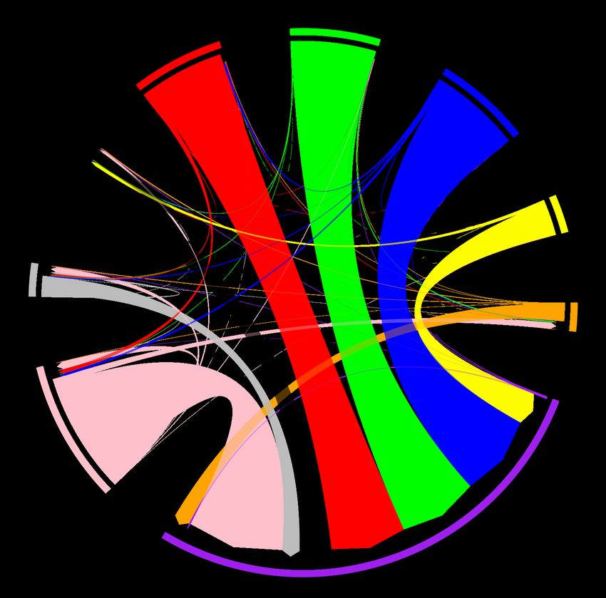
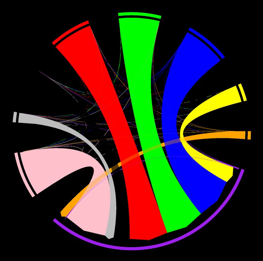
Figure 1: Barge corn shipment origins and river pools

Note: This figure displays the average annual corn tonnage by barge shipment origin. Each river pool is labeled.

 Barge shipments are aggregated within each river pool. Figure 2 displays and Table 1 provides

the flow of average annual barge shipments across all nine river pools between 2000 and 2017. The name

of each river pool is shown on the outer ring. The numbers under the river pool label are the average

annual barge tonnages (in 100,000). Outflows from a river pool are shown with a directional point at the

destination. For example, the figure shows that virtually all barge shipments from the MIDMISS river pool

terminate in the CENTGULF river pool. Nearly all shipments from each river pool end in the CENTGULF

river pool.

 12

Figure 2: Barge corn flows between river pools

 Note: This figure displays the average annual tonnage (in 100,000) shipped and received by barge for each river pool
 from 2000 to 2017. Shipments to a river pool are denoted with an “arrow.”

 Table 1: Average annual barge corn flows between river pools, 2000-17, tons
Origin\Dest CARMEMPH CENTGULF ILLINOIS LOWMISS LOWOHIO MIDMISS STLOUIS UPMISS UPOHIO
CARMEMPH 210 287,601 3,357 786 0 924 844 0 0
CENTGULF 194 33,438 370 2,962 2,228 79 1,119 91 1,125
ILLINOIS 1,025 1,700,000 9,157 83 423 0 1,389 0 380
LOWMISS 0 348,242 5,441 1,157 646 3,513 4,321 0 592
LOWOHIO 501 640,300 99 181 96 0 94 0 213
MIDMISS 264 1,500,000 0 625 1,336 252 706 347 197
STLOUIS 0 1,500,000 169 460 641 0 240 0 352
UPMISS 1,425 1,600,000 616 727 584 1,913 720 681 521
UPOHIO 180 638,238 0 0 197 0 0 0 0

 13

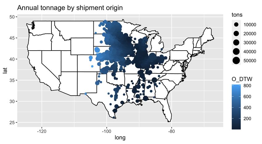
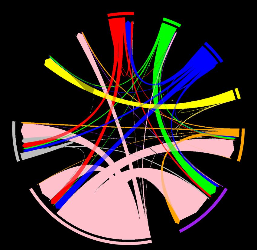
4.2 Rail data

The CWS contains information on rail shipments between all origins and destinations in the United States.

To connect the rail data to the barge data, we start by identifying only rail shipments that terminate in

one of the 9 river pools. For each rail shipment origin, we define the catchment area based on the distance

to the nearest barge location. This forms an origin “zone.” Figure 3 displays all rail shipment origins in

the study region, where the size of the point represents average annual tonnage and the shade represents

the distance to the nearest barge facility. In this paper’s main empirical specification, we initially define

the catchment area as shipments that originate within 100 miles of the waterway. Then, we examine how

the relationships change with different distance bands.

 Figure 3: Rail shipment origins

Note: This figure displays the origins for rail shipments. The size of the point corresponds to the average annual
tonnage, and the color of the port corresponds to the distance to the nearest barge location.

 Figure 4 displays and Table 2 summarizes the average flow of annual rail shipments across all 9

river zones. Similar to Figure 2, the name of the river zones is displayed on the outer ring, and the average

annual tonnage (in 100,000) is displayed below the river zone name. Unlike barge shipments (Figure 2),

rail shipments are more disbursed throughout the 9 river zones. The CENTGULF river pool is not a

 14

significant origin for rail shipments but remains a significant destination. The ILLINOIS river zone is the

most significant origin of rail shipments, with nearly 700,000 tons per year.

 Figure 4: Rail corn flows between river zones

Note: This figure displays the average annual tonnage (in 100,000) shipped and received by rail for each river zone
from 2000 to 2017. Shipments to a river zone are denoted with an “arrow.”

 Table 2: Average annual rail corn flows between river zones, 2000-17, tons
 Origin\Dest CARMEMPH CENTGULF ILLINOIS LOWMISS LOWOHIO MIDMISS STLOUIS UPMISS UPOHIO
 CARMEMPH 1,999 33,995 1,418 10,384 7,116 0 0 0 0
 CENTGULF 0 39 0 137 1,517 0 525 0 0
 ILLINOIS 125,804 250,325 135,571 102,429 45,095 276 8,632 0 421
 LOWMISS 1,219 7,564 3,455 34,336 138 0 0 6 0
 LOWOHIO 2,111 7,986 939 390 224,523 137 545 0 0
 MIDMISS 3,653 13,619 40,943 34,472 397 16,716 1,418 11 0
 STLOUIS 13,480 71,451 1,150 8,352 9,243 301 5 0 0
 UPMISS 8,640 20,062 49,220 20,760 3,278 39,919 3,424 9,202 0
 UPOHIO 54 3,577 0 0 64,593 0 33 0 186

 15

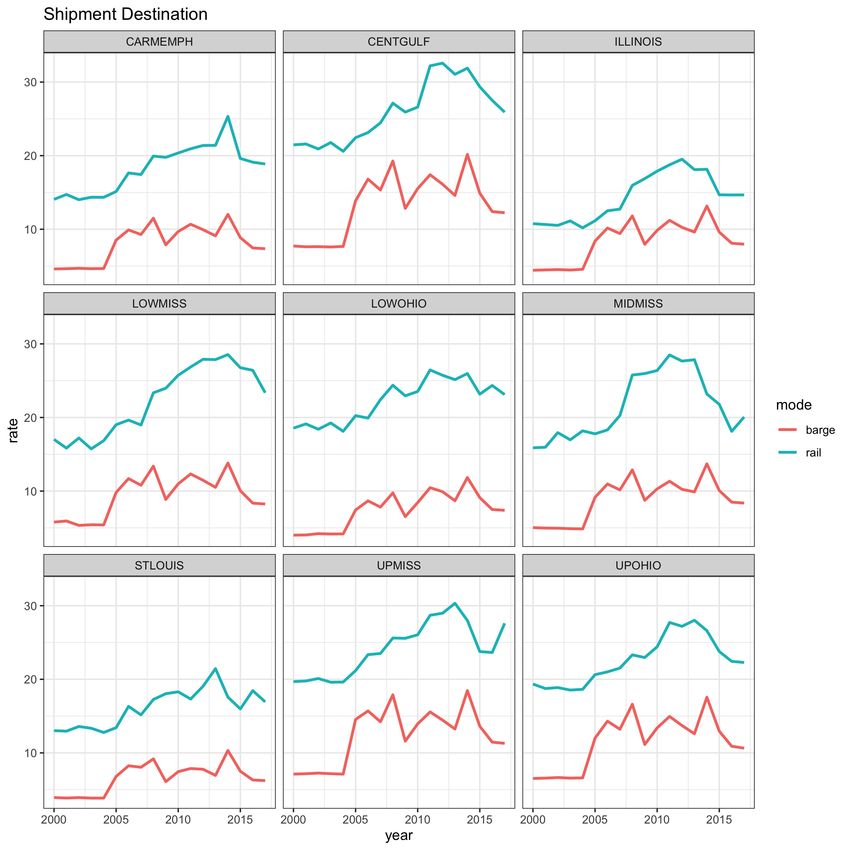
4.3 Combined data

We combined the WCS and CWS data into a single dataset to examine zone to zone movements over time.

The combined dataset contains shipments of corn by rail and barge to all river zones in every year. Figure

5 displays and Table 3 provides the flow of average total tonnage across both modes between all 9 river

zones. This figure is the combination of Figures 2 and 4 and shows the total tonnage shipped between all

river zones in the average year.

 In Figure 6, the share shipped to each terminal zone by origination zone (the dependent variable

in our empirical model) is summarized over time. For all origins, the Central Gulf is the primary

termination location for most points in time. Typically, shares shipped to the Central Gulf are in excess of

80 percent. The shares also vary modestly over time.

 16

Figure 5: Total (barge and rail) corn flows between river zones

Note: This figure displays the average annual tonnage (in 100,000s) shipped and received by barge and rail for each
river zone from 2000 to 2017. Shipments to a river zone are denoted with an “arrow.”

 Table 3: Average total corn flows (barge plus rail) between river zones, 2000-17, tons
 Origin\Dest CARMEMPH CENTGULF ILLINOIS LOWMISS LOWOHIO MIDMISS STLOUIS UPMISS UPOHIO
 CARMEMPH 2,209 321,596 4,775 11,170 7,116 924 844 0 0
 CENTGULF 194 33,477 370 3,098 3,744 79 1,644 91 1,125
 ILLINOIS 126,828 1,900,000 144,728 102,512 45,518 276 10,021 0 802
 LOWMISS 1,219 355,806 8,897 35,493 783 3,513 4,321 6 592
 LOWOHIO 2,611 648,286 1,037 571 224,619 137 639 0 213
 MIDMISS 3,916 1,500,000 40,943 35,098 1,733 16,968 2,124 359 197
 STLOUIS 13,480 1,600,000 1,320 8,812 9,884 301 245 0 352
 UPMISS 10,064 1,700,000 49,836 21,487 3,862 41,832 4,143 9,883 521
 UPOHIO 234 641,815 0 0 64,791 0 33 0 186

 17

Figure 6: Share to each terminal zone by origination zone
 CENTGULF LOWMISS CARMEMPH
1

 1
 1
.8

 .8
 .8
.6

 .6
 .6
.4

 .4
 .4
.2

 .2
 .2
0

 0
 0
 2000 2005 2010 2015 2020 2000 2005 2010 2015 2020 2000 2005 2010 2015 2020
 year year year

 CENTGULF_CENTGULF CENTGULF_CARMEMPH LOWMISS_CENTGULF LOWMISS_CARMEMPH CARMEMPH_CENTGULF CARMEMPH_CARMEMPH
 CENTGULF_ILLINOIS CENTGULF_LOWMISS LOWMISS_ILLINOIS LOWMISS_LOWMISS CARMEMPH_ILLINOIS CARMEMPH_LOWMISS
 CENTGULF_LOWOHIO CENTGULF_MIDMISS LOWMISS_LOWOHIO LOWMISS_MIDMISS CARMEMPH_LOWOHIO CARMEMPH_MIDMISS
 CENTGULF_STLOUIS CENTGULF_UPMISS LOWMISS_STLOUIS LOWMISS_UPMISS CARMEMPH_STLOUIS CARMEMPH_UPMISS
 CENTGULF_UPOHIO LOWMISS_UPOHIO CARMEMPH_UPOHIO

 ILLINOIS LOWOHIO MIDMISS
1

 1
 .8
.8

 .8
 .6
.6

 .6
 .4
.4

 .4
 .2
.2

 .2
0

 0

 0
 2000 2005 2010 2015 2020 2000 2005 2010 2015 2020 2000 2005 2010 2015 2020
 year year year

 ILLINOIS_CENTGULF ILLINOIS_CARMEMPH LOWOHIO_CENTGULF LOWOHIO_CARMEMPH MIDMISS_CENTGULF MIDMISS_CARMEMPH
 ILLINOIS_ILLINOIS ILLINOIS_LOWMISS LOWOHIO_ILLINOIS LOWOHIO_LOWMISS MIDMISS_ILLINOIS MIDMISS_LOWMISS
 ILLINOIS_LOWOHIO ILLINOIS_MIDMISS LOWOHIO_LOWOHIO LOWOHIO_MIDMISS MIDMISS_LOWOHIO MIDMISS_MIDMISS
 ILLINOIS_STLOUIS ILLINOIS_UPMISS LOWOHIO_STLOUIS LOWOHIO_UPMISS MIDMISS_STLOUIS MIDMISS_UPMISS
 ILLINOIS_UPOHIO LOWOHIO_UPOHIO MIDMISS_UPOHIO

 STLOUIS UPMISS UPOHIO

 1
 1
1

 .8
 .8
.8

 .6
 .6
.6

 .4
 .4
.4

 .2
 .2
.2

 0
 0
0

 2000 2005 2010 2015 2020 2000 2005 2010 2015 2020 2000 2005 2010 2015 2020
 year year year

 STLOUIS_CENTGULF STLOUIS_CARMEMPH UPMISS_CENTGULF UPMISS_CARMEMPH UPOHIO_CENTGULF UPOHIO_CARMEMPH
 STLOUIS_ILLINOIS STLOUIS_LOWMISS UPMISS_ILLINOIS UPMISS_LOWMISS UPOHIO_ILLINOIS UPOHIO_LOWMISS
 STLOUIS_LOWOHIO STLOUIS_STLOUIS UPMISS_LOWOHIO UPMISS_MIDMISS UPOHIO_LOWOHIO UPOHIO_MIDMISS
 STLOUIS_STLOUIS STLOUIS_UPMISS UPMISS_STLOUIS UPMISS_UPMISS UPOHIO_STLOUIS UPOHIO_UPMISS
 STLOUIS_UPOHIO UPMISS_UPOHIO UPOHIO_UPOHIO

 18

4.4 Freight Rates

We assembled data on barge and rail rates for corn from two sources. Rail freight rates came from the

CWS to calculate the rate of shipping goods by rail between all 9 river zones. To do this, we use the

weighted average rate (in dollars per ton, adjusted for inflation) across all shipments between origins and

destinations within each river zone. Because this CWS only contains information on shipments that

occurred, the freight rate is missing if there were no shipments between two river zones in a given year.

For example, if there were no shipments that originated within the CENTGULF river zone and terminated

in the ILLINOIS river zone then it is not possible to calculate the rate between CENTGULF and ILLINOIS

using the weighted average. In these cases, we fill in the missing data using an interpolated freight rate

based on the shipping distance.

 Barge rates are calculated using data from USDA’s Agricultural Marketing Service, which contains

information on the annual barge rate (in dollars per ton) between each river pool and the CENTGULF river

pool between 2000 and 2017. We use this data to interpolate barge freight rates between all other river

pools based on the shipping distance. The result is a dataset that contains the yearly barge rate for

shipments between all 9 river pools.

 Figure 7 displays the annual freight rates over time by destination zone and mode. They derive

from a weighted average based on origin zone tonnage and are adjusted for inflation. Barge rates

remained relatively constant over the sample period, while rail rates increased until 2013 and then fell.

The general pattern in freight rates over time is consistent across all river zones. However, the average

barge rate for shipments terminating in the UPOHIO and CENTGULF river zones is higher than in other

destinations. Rail rates for shipments terminating in the CENTGULF river zone are also higher than in other

destinations.

 19

Figure 7: Barge and rail rates

Note: This figure displays the average annual barge and rail rates, in dollars per ton, to each destination.

 20

5. Results

The main results are presented in Table 4. We develop three different specifications and compare the

results to gauge their sensitivity. Model 1 (Column 1) specifies the probability of a choice (choosing a

mode and destination, from a particular origin) as a function of the rate for each option (RATE) and a

dummy variable that indicates that the option involves barge (BARGE). That is, the shipper located at a

given origin chooses the destination and mode based on the rate of each mode to each destination. The

BARGE dummy captures systematic differences between barge and rail. Models 2 and 3 introduce

destination dummy variables, with the omitted category being the CENTGULF zone. These are included

to capture unobserved systematic differences in the destinations. 14 The table's coefficients represent the

parameters of the deterministic part of the utility equation. They reflect the difference in expected

shipper payoffs. The positive sign on BARGE points to a preference for barge. According to the model 1

results, the probability of choosing barge is 5.9 percent higher than rail, on average. Given the positive

sign on RATE in Model 1, Column 2 shows a model with rate and dummy variables for the destination

zones. In this case, RATE is now the expected negative sign (a higher rate lessens the probability a mode

is chosen), which points to the importance of including the terminal destination dummy variables to obtain

unbiased coefficient estimates. Finally, in Column 3, we incorporate the specifications reported in

Columns 1 and 2, which includes the full set of explanatory variables—rate, a dummy for mode, and

dummies for destination.

 Column 3 represents the preferred specification based on likelihood values and expected signs.

In this model, rates can and do have a statistically significant effect. The positive sign on BARGE suggests

that shippers prefer shipping by barge. That is, if barge is a feasible option, shippers tend to choose it

given rates are the same. In addition, in all cases, destinations are associated with lower shipper payoffs

14Due to the extremely small amount of tonnage originating in the CENTGULF region, it is excluded as an origin in the empirical
analysis.

 21

relative to the CENTGULF, which is consistent with the descriptive analysis of the data presented in the

previous section.

 Table 4: Estimation Results
 Model (1) Model (2) Model (3)

 BARGE 5.978*** 2.035***
 (0.675) (0.232)
 RATE 0.271*** -0.221*** -0.080***
 (0.032) (0.015) (0.018)
 CARMEMPH -6.880*** -5.873***
 (0.318) (0.293)
 ILLINOIS -7.642*** -5.728***
 (0.340) (0.286)
 LOWMISS -5.949*** -5.343***
 (0.261) (0.246)
 LOWOHIO -6.393*** -5.156***
 (0.376) (0.343)
 MIDMISS -9.166*** -7.090***
 (0.429) (0.344)
 STLOUIS -10.058** -8.206***
 (0.390) (0.366)
 UPMISS -11.584** -8.909***
 (0.567) (0.450)
 UPOHIO -10.984** -9.724***
 (0.511) (0.370)
 Constant -9.500 2.066 -0.458
 (10.461) (1.402) (1.803)
 Log-Likelihood -378.8 -191.5 -182.7

 The coefficients in Table 4 can be used to calculate conditional choice probabilities, which are

easier to interpret and provide greater insight into the trade-offs between modes and destinations. Figure

8 displays the probability of selecting to ship by barge, conditional on choosing a given destination, based

on the results in Table 4, Column 3. The x-axis displays the barge rate, and the y-axis displays the

conditional choice probabilities of selecting rail or barge. Rail rates are held constant at the destination-

 22

specific average. The result is apparent across all destinations: as barge rates increase, the probability a

shipper chooses to ship by barge falls. The probability that the shipper decides to ship by rail increases as

the barge rate increases. 15

 Figure 8: Modal choice probabilities

Note: This figure displays the mode choice probability, conditional on a destination choice. Rail rates are held
constant at the destination-specific average value.

 Next, we examine how changes to the distance band used to define origins and destinations

influence the results. Figure 9 displays how the coefficient on the barge variable (BARGE) changes when

15Destination choice probabilities can also be calculated from the results in Table 1. For the most part, freight rates do not
have a substantial effect on destination choice probabilities. For barge and rail shipments, the probability of choosing the
CENTGULF region is much higher than the probability of choosing other regions. This makes sense, given the substantial
amount of the Nation’s corn exported out of the region.

 23

the distance band changes. The figure is the result of estimating the specification in Column 3 of Table 1

while allowing the distance band to vary from 50 miles to 300 miles in increments of one mile. Thus, the

figure displays the results from 250 separate regressions. As the distance band increases, the probability

of selecting barge (the coefficient on BARGE) goes down. This suggests the preference for barge declines.

The intuition behind this result is, as shipments originate further from the river are included in the

estimation, the attractiveness of shipping by barge declines.

 Figure 9: Barge effect at different distances

Note: This figure displays the coefficient on the barge dummy variable, and 95% confidence interval, as the distance
band increases from 50 to 300 in increments of 1 mile. The figure shows the results of 250 separate regression
estimates.

 Using similar methods, we examine how the coefficient on the rate variable (RATE) changes. This

is shown in Figure 10. The effect of rates is relatively constant across the different distance bands used in

 24

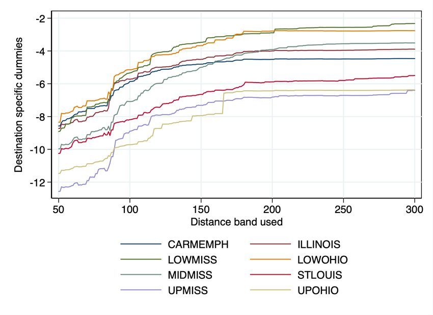
the 250 regressions, especially for distances bands of 175 miles or higher. For all distance bands, except

a distance band of 86 miles, the 95% confidence interval contains the average barge effect of -0.051.

 Figure 10: Rate effect at different distances

Note: This figure displays the coefficient on the rate variable, and 95% confidence interval, as the distance band
increases from 50 to 300 in increments of 1 mile. The figure shows the results of 250 separate regression
estimates.

 Finally, we examine how the destination-specific dummy variables influence shipper payoffs at

different distance bands. The results are displayed in Figure 11. We find that as the distance band used

to determine origins and destinations increases, the payoffs for all destinations increase relative to the

CENTGULF destination (the omitted category). Similar to the results in Figures 9 and 10, at approximately

175 miles, the coefficients stabilize. Further, the rank ordering of the preferences for destinations changes

 25

as the distance band increases. That is, the coefficients estimated for different destinations change in

relative importance. For example, for distance bands between 50 and 90 miles, the payoff associated with

LOWMISS is less than the preference associated with UPOHIO, but as the distance band increases this

relationship flips, so that the preference associated with the LOWMISS is higher than for the UPOHIO.

Similar patterns also exist for other preferences. For example, we find that the preference associated with

MIDMISS increases faster than the ILLINOIS and CARMEMPH destination preference.

 Figure 11: Destination dummies at different distances

Note: This figure displays the coefficient on the destination dummy variables as the distance band increases from
50 to 300 in increments of 1 mile. The figure shows the results of 250 separate regression estimates. The omitted
destination is CENTGULF.

 26

6. Summary and Conclusion

This report provides an in-depth analysis of rail and barge shipments of corn that originate and terminate

within given distances of the Mississippi, Illinois, and Ohio waterways from 2000 to 2017. The research is

framed and executed in terms of demands for movements between locations and modes. The basic tenet

of the research is that the competitive relationship between barge and rail is central to rail pricing

decisions and the calculation of benefits from both public and private infrastructure investment.

 Our analysis bases the construction of pools on the waterway (i.e., a set of locations between

fixed points on the waterway). We used these origin pools, and defined origin zones by incorporating off-

river locations within a given distance. From these origin zones, we aggregate rail shipments within a given

distance band into the origin zone closest and added in the observed barge shipments. Our dependent

variable is the share of origin zone tons shipped to other zones by a given mode. We use the result to

estimate demand models based on a choice framework.

 We find that most corn shipments by barge terminate in the Central Gulf termination zone

(Louisiana), while rail shipments terminate in the Illinois, Central Gulf, and Lower Ohio zones. The

empirical results indicate that the demand flows are affected by rates and terminal dummies (which

capture unobserved effects for each termination zone). We compare estimated probabilities across

termination zones and across modes. For termination zones, the Central Gulf is dominant and remains

dominant over a reasonable range of changes in barge rates. However, the modal choice probabilities do

vary substantially with the level of barge rates.

 The distance band is intended to capture the area in which rail and barge compete for corn traffic.

However, the catchment area is not known beforehand. Instead, we conduct the analysis for a wide range

of distance bands (50 to 300 miles) and compare the results. Generally, we find that there is a preference

for barge, but the preference declines with distance from the waterway. At a distance of 200 miles, there

 27

is no strong preference for barge. The effects of rates also vary with the distance band. With the

exception of a few bands, the estimates are remarkably stable. Finally, we examine the coefficients on

the termination zones over the distance bands. The coefficients for each of the termination zones

increase (from negative values) with the distance bands, and stabilize at a distance of about 175 miles.

 Overall, the results suggest the modal substitution does exist for most observed rates, and the

effect is remarkably stable for most distance bands. However, while there is substitution across

termination zones, it is relatively small.

 To our knowledge, there are no other studies of this type in the modeling of the demand for

freight transportation. The modeling requires the use of distance bands, which reflect the catchment area

for barge movements (the range at which barge is a feasible mode for shippers). In comparing the results

over different distances, it appears that a distance band of about 175 to 200 miles is the most appropriate.

The approach used in this study can be readily adapted for other commodities, and, indeed, offer an

alternative approach to estimating demand elasticities where rail and barge compete.

 The output of the modeling effort is the demand for rail and the demand for barge. Both are of

central interest to policymakers in considering the effects of barge competition on rail prices, which is a

key factor of railroad regulation. In addition, it provides a non-survey approach to estimating barge

demands on the waterway which are consistent with theory. This is important in that the Army Corps of

Engineers generally use a survey approach with discrete choice models to estimate demands. But, this

approach is limited to commodities with a large number of shippers, representative samples, etc.

 In terms of the research's overriding objective, we have carefully examined the linkage between

the demand for barge and rail freight movements and find that the demands are linked over a range of

different barge catchment areas. The results can be implemented for other commodities and used to

gage the impact of pricing and better judge the benefits of both public and private investments.

 28

References

Abdelwahab, Walid M. "Elasticities of mode choice probabilities and market elasticities of demand:
evidence from a simultaneous mode choice/shipment-size freight transport model." Transportation
Research Part E: Logistics and Transportation Review 34, no. 4 (1998): 257-266.

Anderson, Simon P., and Wesley W. Wilson, “Spatial Modeling in Transportation: Congestion and Mode
Choice,” November 1, 2004. IWR Report 04-NETS-P-06. Available on:
http://www.nets.iwr.usace.army.mil/inlandnav.cfm.

Anderson, Simon P., and Wesley W. Wilson. "Spatial competition, pricing, and market power in
transportation: A dominant firm model." Journal of regional science 48, no. 2 (2008): 367-397.

Anderson, Simon P., and Wesley W. Wilson. "Market power in transportation: Spatial equilibrium under
Bertrand competition." Economics of Transportation 4, no. 1-2 (2015): 7-15.

Baumol, William J., and Hrishikesh D. Vinod. "An inventory theoretic model of freight transport demand."
Management science 16, no. 7 (1970): 413-421.

Berry, Steven T. "Estimating discrete-choice models of product differentiation." The RAND Journal of
Economics (1994): 242-262.

Berry, Steven, James Levinsohn, and Ariel Pakes. "Automobile prices in market equilibrium."
Econometrica: Journal of the Econometric Society (1995): 841-890.

Boyer, Kenneth D., and Wesley W. Wilson, “Estimation of Demands at the Pool Level,” March 14, 2005,
IWR Report 05-NETS-R-03, Available on http://www.nets.iwr.usace.army.mil/inlandnav.cfm

Burton, Mark L. "Railroad deregulation, carrier behavior, and shipper response: A disaggregated analysis."
Journal of Regulatory Economics 5, no. 4 (1993): 417-434.

Burton, Mark, and Wesley W. Wilson. "Network pricing: Service differentials, scale economies, and vertical
exclusion in railroad markets." Journal of Transport Economics and Policy (JTEP) 40, no. 2 (2006): 255-277.

Clark, Chris, Helen T. Naughton, Bruce Proulx, and Paul Thoma 2005. “A survey of the freight
transportation demand literature and a comparison of elasticity estimates”. Institute for Water Resources
US Army Corps of Engineers, IWR Report 05-NETS-R-01, Alexandria, Virginia.

Henrickson, Kevin E., and Wesley W. Wilson. "Model of spatial market areas and transportation demand."
Transportation research record 1909, no. 1 (2005a): 31-38.

Henrickson, K., and W. Wilson. "Patterns in Geographic Elasticity Estimates of Barge Demand on the Upper
Mississippi and Illinois Rivers." The Transportation Research Record: Journal of the Transportation
Research Board (2005b).

Inaba, Fred S., and Nancy E. Wallace. "Spatial price competition and the demand for freight
transportation." The Review of Economics and Statistics (1989): 614-625.

 29

MacDonald, James M. "Competition and rail rates for the shipment of corn, soybeans, and wheat." The
Rand Journal of Economics (1987): 151-163

MacDonald, James M. "Railroad deregulation, innovation, and competition: Effects of the Staggers Act on
grain transportation." The Journal of Law and Economics 32, no. 1 (1989): 63-95.

McFadden (1973), Daniel L. “Conditional Logit Analysis of Qualitative Choice Behavior” in Frontiers in
Econometrics, ed. by P. Zarembka, Wiley, New York.

Nevo, Aviv. "A practitioner's guide to estimation of random‐coefficients logit models of demand." Journal
of economics & management strategy 9, no. 4 (2000): 513-548.

Quandt, Richard E., and William J. Baumol. "The demand for abstract transport modes: theory and
measurement." The Collected Essays of Richard E. Quandt 1, no. 2 (1992): 275.

Train, Kenneth, and Wesley W. Wilson, “Shippers’ Responses to Changes in Transportation Rates and
Times: The Mid-American Grain Study,” November 1, 2004, IWR Report 04-NETS-R-02. Available on:
http://www.nets.iwr.usace.army.mil/inlandnav.cfm .

Train, Kenneth, and Wesley W. Wilson (2006). Spatial Demand Decisions in the Pacific Northwest: Mode
Choices and Market Areas. Transportation Research Record: Journal of the Transportation Research Board
No. 1963, pp. 9-14.

Train, Kenneth, and Wesley W. Wilson, “Transportation Demands in the Columbia-Snake River Basin,”
March 1, 2006, IWR Report 06-NETS-R-03. Available on:
http://www.nets.iwr.usace.army.mil/inlandnav.cfm .

Train, Kenneth, and Wesley W. Wilson. "Spatially generated transportation demands." Research in
Transportation Economics 20 (2007): 97-118.

Train, Kenneth, and Wesley W. Wilson, “Transportation Demand for Agricultural Products in the Upper
Mississippi and Illinois River Basin”, IWR Report 07-NETS-R-2, May 2007.

Train, Kenneth, and Wesley W. Wilson (2008). "Transportation Demand and Volume Sensitivity: A Study
of Grain Shippers in the Upper Mississippi River Valley." Transportation Research Record No. 2062. pp.
66-73.

Train, Kenneth, and Wesley W. Wilson (2008) “Estimation on Stated-Preference Experiments Constructed
from Revealed-Preference Choices." Transportation Research – B, Vol. 42 (2008), 191-2003.

Train, Kenneth, and Wesley W. Wilson (2009). "Monte Carlo Analysis of SP-off-RP Data." Journal of Choice
Modeling. Vol. 2(1), 101-117.

Train, Kenneth and Wesley W. Wilson, “Demand for the Transportation of Agricultural Products: An
Application to Shippers in the Upper Mississippi and Illinois River Basins”. Report to the US Army Corps
of Engineers, October, 2019.

 30

Winston, Clifford. "The demand for freight transportation: models and applications." Transportation
Research Part A: General 17, no. 6 (1983): 419-427.

Winston, Clifford. "Conceptual developments in the economics of transportation: an interpretive survey."
Journal of Economic Literature 23, no. 1 (1985): 57-94.

 31

Appendix: Modeling Shipper Decisions

The random utility model offers a useful framework to examine shipper decisions and it has been used

extensively to model mode choice. In the present case, shipper i chooses to ship to a terminal location j

by a given mode m. Given a set of alternatives, individuals select the option that provides them with the

highest utility. Utility for each shipper and option (terminal and mode combination) is taken to consist of

two components—a deterministic component (Vijm) and a random component ( ) and is given by:

 = + (A-1)

 In equation (A-1), Vijm represents the systematic, measurable component of utility. The term is

an unmeasurable component that is unique to each shipper. We assume the unobservable terms are

drawn from an independent and identically distributed extreme value distribution. Under this

assumption, the probability shipper i chooses destination j by mode m can be estimated with a logit model.

The probability of a choice is given by:

 = ∑ (A-2)
 
where Vijm is the measurable component of shipper utility. The next step is to specify the deterministic

portion. In our case, we specify the deterministic part (V) as a function of freight rates and a set of

alternative specific dummies including the mode and the terminal locations. Suppressing the observation

index i, this specification is as:

 = 1 + 2 + 2 (A-3)

where, Bargeij is a dummy variable that corresponds barge shipments between i and j and Destj is a set of

destination dummies that which control for destination-specific unobservable factors (e.g., prices of the

commodity, the level of demand for the product shipped, etc.).

 In equation (A-3), shipments by barge to a destination by a mode are each observed. The function

is substituted into equation (A-2) and the unknown parameter estimated by maximum likelihood. In our

 32

case, the dependent variable is not the choice, but rather the share tonnages that originate in origination

zone (i) and travels to terminal zone (j) by mode(m).

 33