Fair Selective Classification via Sufficiency - Proceedings of ...
←
→
Page content transcription
If your browser does not render page correctly, please read the page content below
Fair Selective Classification via Sufficiency

 Yuheng Bu * 1 Joshua Ka-Wing Lee * 1 Subhro Das 2 Rameswar Panda 2 Deepta Rajan 2 Prasanna Sattigeri 2
                                           Gregory Wornell 1

                          Abstract                              The field of fair machine learning is rich with both problems
                                                                and proposed solutions, aiming to provide unbiased decision
      Selective classification is a powerful tool for           systems for various applications. A number of different
      decision-making in scenarios where mistakes are           definitions and criteria for fairness have been proposed, as
      costly but abstentions are allowed. In general, by        well as a variety of settings where fairness might be applied.
      allowing a classifier to abstain, one can improve
      the performance of a model at the cost of reducing        One major topic of interest in fair machine learning is that
      coverage and classifying fewer samples. However,          of fair classification, whereby we seek to make a classifier
      recent work has shown, in some cases, that selec-         “fair” for some definition of fairness that varies according
      tive classification can magnify disparities between       to the application. In general, fair classification problems
      groups, and has illustrated this phenomenon on            arise when we have protected groups that are defined by a
      multiple real-world datasets. We prove that the           shared sensitive attribute (e.g., race, gender), and we wish
      sufficiency criterion can be used to mitigate these       to ensure that we are not biased against any one group with
      disparities by ensuring that selective classification     the same sensitive attribute.
      increases performance on all groups, and intro-           In particular, one sub-setting of fair classification which
      duce a method for mitigating the disparity in preci-      exhibits an interesting fairness-related phenomenon is that
      sion across the entire coverage scale based on this       of selective classification. Generally speaking, selective
      criterion. We then provide an upper bound on the          classification is a variant of the classification problem where
      conditional mutual information between the class          a model is allowed to abstain from making a decision. This
      label and sensitive attribute, conditioned on the         has applications in settings where making a mistake can be
      learned features, which can be used as a regular-         very costly, but abstentions are not (e.g., if the abstention
      izer to achieve fairer selective classification. The      results in deferring classification to a human actor).
      effectiveness of the method is demonstrated on the
      Adult, CelebA, Civil Comments, and CheXpert               In general, selective classification systems work by assign-
      datasets.                                                 ing some measure of confidence about their predictions,
                                                                and then deciding whether or not to abstain based on this
                                                                confidence, usually via thresholding.

1. Introduction                                                 The desired outcome is obvious: the higher the confidence
                                                                threshold for making a decision (i.e., the more confident
As machine learning applications continue to grow in scope      one needs to be to not abstain), the lower the coverage
and diversity, its use in industry raises increasingly many     (proportion of samples for which a decision is made) will
ethical and legal concerns, especially those of fairness and    be. But in return, one should see better performance on the
bias in predictions made by automated systems (Selbst et al.,   remaining samples, as the system is only making decisions
2019; Bellamy et al., 2018; Meade, 2019). As systems are        when it is very sure of the outcome. In practice, for most
trusted to aid or make decisions regarding loan applications,   datasets, with the correct choice of confidence measure and
criminal sentencing, and even health care, it is more impor-    the correct training algorithm, this outcome is observed.
tant than ever that these predictions be free of bias.
                                                                However, recent work has revealed that selective classifica-
  *
    Equal contribution 1 Department of Electrical Engineering   tion can magnify disparities between groups as the coverage
and Computer Science, Massachusetts Institute of Technology,    decreases, even as overall performance increases. (Jones
Cambridge, USA 2 MIT-IBM Watson AI Lab, IBM Research,           et al., 2020). This, of course, has some very serious con-
Cambridge, USA. Correspondence to: Joshua Ka-Wing Lee .                                             sequences for systems that require fairness, especially if it
                                                                appears at first that predictions are fair enough under full
Proceedings of the 38 th International Conference on Machine    coverage (i.e., when all samples are being classified).
Learning, PMLR 139, 2021. Copyright 2021 by the author(s).
Fair Selective Classification Via Sufficiency
Thus, we seek a method for enforcing fairness which ensures repaying a loan (Y ) given factors about one’s financial situa-
that a classifier is fair even if it abstains from classifying on tion (X) should not be determined by gender (D). While D
a large number of samples. In particular, having a measure can be continuous or discrete (and our method generalizes
of confidence that is reflective of accuracy for each group to both cases), we focus in this paper on the case where
can ensure that thresholding doesn’t harm one group more D is discrete, and refer to members which share the same
than another. This property can be achieved by applying value of D as being in the same group. This allows us to
a condition known as sufficiency, which ensures that our formulate metrics based on group-specific performance.
predictive scores in each group are such that they provide
There are numerous metrics and criteria for what constitutes
the same accuracy at each confidence level (Barocas et al.,
a fair classifier, many of which are mutually exclusive with
2019). This condition also ensures that the precision on
one another outside of trivial cases. One important criteria
all groups increases when we apply selective classification,
is positive predictive parity (Corbett-Davies et al., 2017;
and can help mitigate the disparity between groups as we
Pessach & Shmueli, 2020), which is satisfied when the pre-
decrease coverage.
cision (which we denote as P P V , after Positive Predictive
The sufficiency criteria can be formulated as enforcing a Value) for each group is the same, that is:
conditional independence between the label and sensitive
attribute, conditioned on the learned features, and thus al- ∀a, b ∈ D, P(Y = 1|Ŷ = 1, D = a) = P(Y = 1|Ŷ = 1, D = b).
lows for a relaxation and optimization method that centers (1)
around the mutual information. However, to impose this This criteria is especially important in applications where
criteria, we require the use of a penalty term that includes false positives are particularly harmful (e.g., criminal sen-
the conditional mutual information between two discrete tencing or loan application decisions) and having one group
or continuous variables conditioned on a third continuous falsely labeled as being in the positive group could lead to
variable. Existing method for computing the mutual infor- great harm or contribute to further biases. Looking at preci-
mation for the purposes of backpropagation tend to struggle sion rates can also reveal disparities that may be hidden by
when the term in the condition involves the learned features. only considering the differences in accuracies across groups
In order to facilitate this optimization, we thus derive an (Angwin et al., 2016).
upper-bound approximation of this quantity.
When D is binary, an intuitive way to measure the severity
In this paper, we make two main contributions. Firstly, we of violations of this condition is to measure the difference
prove that sufficiency can be used to train fairer selective in precision between the two groups:
classifiers which ensure that precision always increases as
coverage is decreased for all groups. Secondly, we derive ∆P P V , P(Y = 1|Ŷ = 1, D = 0)−P(Y = 1|Ŷ = 1, D = 1).
a novel upper bound of the conditional mutual information (2)
which can be used as a regularizer to enforce the sufficiency
criteria, then show that it works to mitigate the disparities A number of methods exist for learning fairer classifiers.
on real-world datasets. (Calders et al., 2009) and (Menon & Williamson, 2018)
reweight probabilities to ensure fairness, while (Zafar et al.,
2017) proposes using covariance-based constraints to en-
2. Background force fairness criteria, and (Zhang et al., 2018) uses an
2.1. The Fair Classification Problem adversarial method, requiring the training of an adversarial
classifier. Still others work by directly penalizing some spe-
We begin with the standard supervised learning setup of cific fairness measure (Zemel et al., 2013b; du Pin Calmon
predicting the value of a target variable Y ∈ Y using a set et al., 2017).
of decision or predictive variables X ∈ X with training
samples {(x1 , y1 ), . . . , (xn , yn )}. For example, X may be Many of these methods also work by penalizing some ap-
information about an individual’s credit history, and Y is proximation or proxy for the mutual information. (Mary
whether the individual will pay back a certain loan. In et al., 2019; Baharlouei et al., 2020; Lee et al., 2020) propose
general, we wish to find features Φ(x) ∈ RdΦ , which are the use of the Hirschfeld-Gebelein-Renyi maximal corre-
predictive about Y , so that we can construct a good predictor lation as a regularizer for the independence and separation
ŷ = T (Φ(x)) of y under some loss criteria L(ŷ, y), where constraints (which requires that Ŷ ⊥ D and Ŷ ⊥ D | Y ,
T denotes the final classifier on the learned features. respectively), which has been shown to be an approximation
for the mutual information (Huang et al., 2019). Finally,
Now suppose we have some sensitive attributes D ∈ D we (Cho et al., 2020) approximates the mutual information us-
wish to be “fair” about (e.g., race, gender), and training sam- ing a variational approximation. However, none of these
ples {(x1 , y1 , d1 ), . . . , (xn , yn , dn )}. For example, in the methods are designed to tackle the selective classification
banking system, predictions about the chance of someone problem.Fair Selective Classification Via Sufficiency
2.2. Selective Classification
In selective classification, a predictive system is given the
choice of either making a prediction Ŷ or abstaining from
the decision. The core assumption underlying selective clas-
sification is that there are samples for which a system is
more confident about its prediction, and by only making
predictions when it is confident, the performance will be
improved. To enable this, we must have a confidence score
κ(x) which represents the model’s certainty about its pre-
diction on a given sample x (Geifman & El-Yaniv, 2017).
Then, we threshold on this value to decide whether to make
a decision or to abstain. We define the coverage as the frac-
tion of samples for which we do not abstain on (i.e., the
fraction of samples that we make predictions on).
As is to be expected, when the confidence is a good measure
of the probability of making a correct prediction, then as
we increase the minimum confidence threshold for making
the prediction (thus decreasing the coverage), we should see
the risk on the classified samples decrease or the accuracy
over the classified samples increase. This leads us to the Figure 1. (Top) When margin distributions are not aligned, (Bot-
accuracy-coverage tradeoff, which is central to selective tom) then as we sweep over the threshold τ , the accuracies for the
classification (though we note here the warning from the groups do not necessarily move in concert with one another.
previous section about accuracy not telling the whole story).
Selective classifiers can work a posteriori by taking in an on the worst-case group.
existing classifier and deriving an uncertainty measure from
it for which to threshold on (Geifman & El-Yaniv, 2017), In general, this phenomenon occurs due to a difference be-
or a selective classifier can be trained with an objective that tween the average margin distribution and the group-specific
is designed to enable selective classification (Cortes et al., margin distributions, resulting in different levels of perfor-
2016; Yildirim et al., 2019). mance when thresholding, as illustrated in Figure 1.
One common method of extracting a confidence score from The margin M of a classifier is defined as κ(x) when
an existing network is to take the softmax response s(x) as ŷ(x) = y and −κ(x) otherwise. If we let τ be our threshold,
a measure of confidence. In the case of binary classification, then a selective classifier makes the correct prediction when
to better visualize the distribution of the scores, we define M (x) ≥ τ and incorrect predictions when M (x) ≤ −τ .
the confidence using a monotonic mapping of s(x): We also denote its probability density function (PDF) and
cumulative density function (CDF) as fM and FM , respec-
1 s(x) tively. Then, the selective accuracy is
κ = log (3)
2 1 − s(x)
1 − FM (τ )
which maps [0.5, 1] to [0, ∞] and provides much higher AF (τ ) = (4)
FM (−τ ) + 1 − FM (τ )
resolution on the values close to 1.
for a given threshold. We can analogously compute the
Finally, to measure the effectiveness of selective classifi-
selective precision by conditioning on Ŷ = 1,
cation, we can plot the accuracy-coverage curve, and then
compute the area under this curve to encapsulate the perfor- 1 − FM |Ŷ =1 (τ )
mance across different coverages (Franc & Průša, 2019). P P VF (τ ) = . (5)
FM |Ŷ =1 (−τ ) + 1 − FM |Ŷ =1 (τ )
2.3. Biases in Selective Classification We can also analogously define the distributions of the mar-
gin for each group using fM,D and FM,d for group d ∈ D.
(Jones et al., 2020) has shown that in some cases, when cov-
erage is decreased, the difference in recall between groups (Jones et al., 2020) proposes a number of different situa-
can sometimes increase, magnifying disparities between tions for which average accuracy could increase but worst-
groups and increasing unfairness. In particular, they have group accuracy could decrease based on their relative mar-
shown that in the case of the CelebA and CivilComments gin distributions. For example, if F is left-log-concave
dataset, decreasing the coverage can also decrease the recall (e.g., Gaussian), then AF (τ ) is monotonically increasingFair Selective Classification Via Sufficiency
when AF (0) ≥ 0.5 and monotonically decreasing other- From this, we can guarantee that as we sweep through the
wise. Thus, if AF (0) > 0.5 but AFd (0) < 0.5, then average threshold, we will never penalize performance of any one
accuracy may increase as we increase τ (and thus decrease group in service of increasing the overall precision. Fur-
coverage) but the accuracy on group d may decrease, thus thermore, in most real-world applications, the precision on
resulting in magnified disparity. This same phenomenon the best-performing groups tends to saturate very quickly
occurs with the precision when we condition on Ŷ = 1. In to values close to 1 when coverage is reduced, and thus, if
general, when margin distributions are not aligned between we can guarantee that the precision increases on the worst
groups, disparity can increase as one sweeps over the thresh- performing group as well, then in general, the difference in
old τ . Further subdividing groups according to their label precision between groups decreases as coverage decreases.
yields the difference in recall rates observed.
3.2. Imposing the Sufficiency Condition
3. Fair Selective Classification with From the above theorem, we can see that the classifier given
Sufficiency by the following optimization problem which satisfies suf-
ficiency should yield the desired property of enabling fair
3.1. Sufficiency and Fair Selective Classification
selective classification. It should ensure that as we sweep
Our solution to the fair selective classification problem is to over the coverage, the performance of one group is not
apply the sufficiency criteria to the learned features. penalized in the service of improving the performance of
another group or improving the average performance.
Sufficiency requires that Y ⊥ D | Ŷ or Y ⊥ D | Φ(X), i.e.,
the prediction completely subsumes all information about min L(ŷ, y)
θ
the sensitive attribute that is relevant to the label (Cleary, (8)
1966). When Y is binary, the sufficiency criteria requires s.t. Y ⊥ D|Φ(X),
that (Barocas et al., 2019): where ŷ = T (Φ(x)), and θ are the model parameters for
both Φ and T . One possible way of representing the suffi-
P(Y = 1|Φ(x), D = a) = P(Y = 1|Φ(x), D = b),
ciency constraint is by using the mutual information:
∀a, b ∈ D. (6)
min L(ŷ, y)
Sufficiency has applications to full-coverage positive pre- θ
(9)
dictive parity, and is also used for solving the domain gener- s.t. I(Y ; D|Φ(X)) = 0.
alization problem by learning domain-invariant features, as
in Invariant Risk Minimization (IRM) (Creager et al., 2020; This follows from the fact that Y ⊥ D | Φ(X) is satisfied
Arjovsky et al., 2019). if and only if I(Y ; D|Φ(X)) = 0. This provides us with a
simple relaxation of the constraint into the following form:
The application of this criteria to fair selective classification
comes to us by way of Calibration by Group. Calibration min L(ŷ, y) + λI(Y ; D|Φ(X)). (10)
θ
by group (Chouldechova, 2017) requires that there exists a
score function R = s(x) such that, for all r ∈ (0, 1): We note here that existing works using mutual information
for fairness are ill-equipped to handle this condition, as they
P(Y = 1|R = r, D = a) = r, ∀a ∈ D. (7) assume that it is not the features that will be conditioned
The following result from (Barocas et al., 2019) links cali- on, but rather that the penalty will be the mutual informa-
bration and sufficiency: tion between the sensitive attribute and the features (e.g.,
penalizing I(Φ(X); D) for demographic parity), possibly
Theorem 1. If a classifier has sufficient features Φ, then conditioned on the label (e.g., penalizing I(Φ(X); D|Y )
there exists a mapping h(T (Φ)) : [0, 1] → [0, 1] such that in the case of equalized odds). As such, existing methods
h(T (Φ)) is calibrated by group. either assume that the variable being conditioned on is dis-
If we can find sufficient features Φ(X), so that the score crete (du Pin Calmon et al., 2017; Zemel et al., 2013a; Hardt
function is calibrated by group based these features, then et al., 2016), become unstable when the features are placed
we have the following result (the proof can be found in the in the condition (Mary et al., 2019), or simply do not allow
Appendix A): for conditioning of this type due to their formulation (Grari
et al., 2019; Baharlouei et al., 2020).
Theorem 2. If a classifier has a score function R = s(x)
which is calibrated by group, and selective classification is Thus, in order to approximate the mutual information for
performed using confidence κ as defined in (3), then for all our purposes, we must first derive an upper bound for the
groups d ∈ D we have that both AF (τ ) and P P VFd (τ ) are mutual information which is computable in our applications.
monotonically increasing with respect to τ . Furthermore, Our bound is inspired by the work of (Cheng et al., 2020)
we also have that AFd (0) > 0.5 and P P VFd (0) > 0.5. and is stated in the following theorem:Fair Selective Classification Via Sufficiency
Theorem 3. For random variables X, Y and Z, we have Algorithm 1 Training with sufficiency-based regularizer
Data: Training samples {(x1 , y1 , d1 ), . . . , (xn , yn , dn )},
IUB (X; Y |Z) ≥ I(X; Y |Z), (11)
{de1 , . . . , den }, which are drawn i.i.d. from the em-
where equality is achieved if and only if X ⊥ Y | Z, and pirical distribution P̂D
Initialize Φ, T (parameterized by θφ and θT , respectively)
IUB (X; Y |Z) , EPXY Z [log P (Y |X, Z)] and θd with pre-trained model, and let nd be the number
(12)
− EPX [EPY Z [log P (Y |X, Z)]] . of samples in group d.
Compute the following losses: P
Proof. The conditional mutual information can be written Group-specific losses Ld = − i: di =d log q(yi |Φ(xi ); θ)
Pn
as Joint loss L0 = n1 i=1 L T (Φ(xi )), yi
Regularizer loss LR defined in (17) including both Group-
I(X; Y |Z)
specific loss and Group-agnostic loss
= EPXY Z [log P (Y |X, Z)] − EPY Z [log P (Y |Z)] . (13) for each training iteration do
Thus, for d = 1, . . . , |D| do // Fit group-specific
models
IUB (X; Y |Z) − I(X; Y |Z) for j = 1, . . . , M do // For each batch
= EPY Z [log P (Y |Z) + EPX [− log P (Y |X, Z)]] . (14) θd ← θd − n1d ηd ∇θ Ld
end
Note that − log(·) is convex, end
EPX [− log P (Y |X, Z)] ≥ − log EPX [P (Y |X, Z)] for j = 1, . . . , N do // For each batch
θφ ← θφ − n1 ηf ∇θφ (L0 + λLR ) // Update
= − log P (Y |Z), (15)
feature extractor
which completes the proof. θT ← θT − n1 η∇θT L0 // Update joint
classifier
Thus, I(Y ; D|Φ(X)) can be upper bounded by IUB as: end
end
I(Y ; D|Φ(X)) ≤ EPXY D [log P (Y |Φ(X), D)] (16)
− EPD [EPXY [log P (Y |Φ(X), D)]] .
where dei are drawn i.i.d. from the marginal distribution PD ,
Since P (y|Φ(x), d) is unknown in practice, we need to use and for d ∈ D,
a variational distribution q(y|Φ(x), d; θ) with parameter θ X
to approximate it. Here, we adopt a neural net that predicts θd = arg max log q(yi |Φ(xi ); θ). (18)
θ
Y based on feature Φ(X) and sensitive attribute D as our i: di =d
variational model q(y|Φ(x), d; θ).
Let T denote a joint classifier over all groups which is used
However, in many cases, X will be continuous, high- to make final predictions, such that ŷ = T (Φ(x)), then the
dimensional data (e.g., images), while D will be a discrete, overall loss function is
categorical variable (e.g., gender, ethnicity). Therefore, it n
1 X
would be more convenient to instead formulate the model as min L T (Φ(xi )), yi + λ log q(yi |Φ(xi ); θdi )
θT ,θΦ n
q(y|Φ(x); θd ), i.e., to train a group-specific model for each i=1
d ∈ D to approximate P (y|Φ(x), d), instead of treating D
− λ log q(yi |Φ(xi ); θdei ) . (19)
as a single input to the neural net.
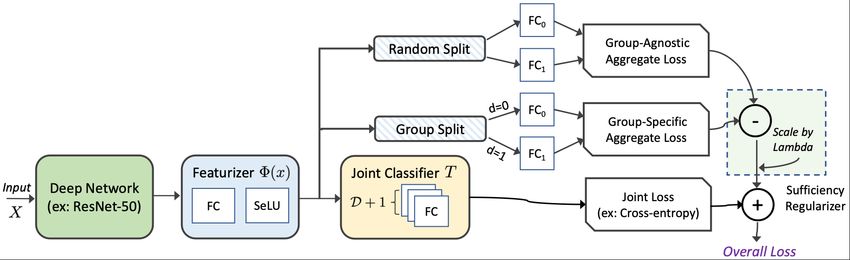
Then, we can compute the first term of the upper bound In practice, we train our model by alternating between the
as the negative cross-entropy of the training samples using fitting steps in (18) and feature updating steps in (19), and
the “correct” classifier for each group (group-specific loss), the overall training process is described in Algorithm 1 and
and the second term as the cross-entropy of the samples Figure 2. Intuitively, by trying to minimize the difference
using a randomly-selected classifier (group-agnostic loss) between the log-probability of the output of the correct
drawn according to the marginal distribution PD . Thus, by model and that of the randomly-chosen one, we are trying
replacing all expectations in (16) with empirical averages, to enforce Φ(x) to have the property that all group-specific
the regularizer is given by models trained on it will be the same; that is:
n
1 X q(y|Φ(x); θa ) = q(y|Φ(x); θb ), ∀a, b ∈ D. (20)
LR , log q(yi |Φ(xi ); θdi )−log q(yi |Φ(xi ); θdei ) ,
n i=1 This happens when P (Y |Φ(X), D) = P (Y |Φ(X)), which
(17) implies the sufficiency condition Y ⊥ D|Φ(X).Fair Selective Classification Via Sufficiency
Figure 2. Diagram illustrating the computation of our sufficiency-based loss when D is binary.
Table 1. Summary of datasets.
Dataset Modality Target Attribute
Adult Demographics Income Sex
CelebA Photo Hair Gender
Colour
Civil Com- Text Toxicity Christianity
ments
CheXpert- X-ray Disease Support
device Device
4. Experimental Results Figure 3. Overall accuracy-coverage curves for Adult dataset for
the three methods.
4.1. Datasets and Setup
We test our method on four binary classification datasets
(while our method works with multi-class classification the sensitive attribute D. In order to simulate the bias phe-
in general, our metrics for comparison are based on the nomenon discussed in Section 2.3, we also drop all but the
binary case), which are commonly used in fairness: Adult1 , first 50 samples for which D = 0 and Y = 1. We then use a
CelebA2 , Civil Comments3 , and CheXpert4 . In all cases, two-layer neural network with 80 nodes in the hidden layer
we use the standard train/val/test splits packaged with the for classification, as in (Mary et al., 2019), with the first
datasets and implemented our code in PyTorch. We set λ = layer serving as the feature extractor and the second as the
0.7 for all datasets as well, which we chose by sweeping classifier, and trained the network for 20 epochs.
over values of λ across all datasets. The CelebA dataset (Liu et al., 2015) consists of 202,599
The Adult dataset (Kohavi, 1996) consists of census data images of 10,177 celebrities, along with a list of attributes
drawn from the 1994 Census database, with 48,842 sam- associated with them. As in (Jones et al., 2020), we use the
ples. The data X consists of demographic information about images as data X (resized to 224x224), the hair color (blond
individuals, including age, education, marital status, and or not) as the target label Y , and the gender as the sensitive
country of origin. Following (Bellamy et al., 2018), we one- attribute D, then train a ResNet-50 model (He et al., 2016)
hot encode categorical variables and designate the binary- (with initialization using pre-trained ImageNet weights) for
quantized income to be the target label Y and sex to be 10 epochs on the dataset, with the penultimate layer as the
feature extractor and the final layer as the classifier.
1
https://archive.ics.uci.edu/ml/datasets/adult
2
http://mmlab.ie.cuhk.edu.hk/projects/CelebA.html The Civil Comments dataset (Borkan et al., 2019) is a text-
3
https://www.kaggle.com/c/jigsaw-unintended-bias-in- based dataset consisting of a collection of online comments,
toxicity-classification/data numbering 1,999,514 in total, on various news articles,
4
https://stanfordmlgroup.github.io/competitions/chexpert along with metadata about the commenter and a label in-Fair Selective Classification Via Sufficiency
(a) Baseline (b) DRO (c) Sufficiency-regularized
Figure 4. Group-specific precision-coverage curves for Adult dataset for the three methods.
(a) Baseline (b) DRO (c) Sufficiency-regularized
Figure 5. Group-specific precision-coverage curves for CheXpert dataset for the three methods.
dicating whether the comment displays toxicity or not. As et al., 2020).
in (Jones et al., 2020), we let X be the text of the com-
ment, Y be the toxicity binary label, and D to be mention of 4.2. Results and discussion
Christianity. We pass the data first through a BERT model
(Devlin et al., 2019) with Google’s pre-trained parameters Figure 3 shows the overall accuracy vs. coverage graphs for
(Turc et al., 2019) and treat the output features as the input each method on the Adult dataset. We can see that, in all
into our system. We then apply a two-layer neural network cases, selective classification increases the overall accuracy
to the BERT output with 80 nodes in the hidden layer, once on the dataset, as is to be expected.
again treating the layers as feature extractor and classifier, However, when we look at the group-specific precisions
respectively. We trained the model for 20 epochs. in Figure 4, we observe that, for the baseline method, this
The CheXpert dataset (Irvin et al., 2019) comprises of increase in performance comes at the cost of worse per-
224,316 chest radiograph images from 65,240 patients with formance on the worst-case group. This phenomenon is
annotations for 14 different lung diseases. As in (Jones heavily mitigated in the case of DRO, but there is still a
et al., 2020), we consider the binary classification task of gap in performance in the mid-coverage regime. Finally,
detecting Pleural Effusion (PE). We set X to be the X-ray our method shows the precisions converging to equality as
image of resolution 224x224, Y is whether the patient has coverage decreases very quickly. This can be explained by
PE, and D is the presence of a support device. We train a looking at the margin distributions for each method. The
model by fine-tuning the DenseNet-121 (Huang et al., 2017) margin distribution histograms are plotted in Figure 6. We
(with initialization using pre-trained ImageNet weights) for can see that the margin distributions are mismatched for the
10 epochs on the dataset, with the penultimate layer as the two groups in the baseline and DRO cases, but aligned for
feature extractor and the final layer as the classifier. our sufficiency-based method.
We compared our results to a baseline where we only op- Figure 5 and 7 show the group precisions and margin dis-
timize the cross-entropy loss, as in standard classification. tributions for the CheXpert dataset. We can see that our
We also compared our method to the group DRO method of method produces a smaller gap in precision at almost all
(Sagawa et al., 2019), using the code provided publicly on coverages compared to the other two methods, and improves
Github5 , which has been shown to mitigate the disparity in the worst-group precision. Note, in this use-case the pres-
recall rates between groups in selective classification (Jones ence of a support device (e.g., chest tubes) is spuriously
correlated to being diagnosed as having PE (Oakden-Rayner
5
https://github.com/kohpangwei/group DRO et al., 2020). Thus, the worst-case group includes X-raysFair Selective Classification Via Sufficiency
(a) Baseline (b) DRO (c) Sufficiency-regularized
Figure 6. Margin distributions for Adult dataset for the three methods.
(a) Baseline (b) DRO (c) Sufficiency-regularized
Figure 7. Margin distributions for CheXpert dataset for the three methods.
this, it is clear that while our method may incur a small
Table 2. Area under curve results for all datasets.
decrease in overall accuracy in some cases, it reduces the
disparity between the two groups, as desired.
Dataset Method Area under Area between
accuracy precision More experimental results can be found in Appendix B for
curve curves additional baselines on the Adult Dataset, as well as the
precision-coverage curves and margin distributions for the
Adult Baseline 0.931 0.220
CelebA and CivilComments datasets.
DRO 0.911 0.116
Ours 0.887 0.021
5. Conclusion
CelebA Baseline 0.852 0.094
DRO 0.965 0.018 Fairness in machine learning has never been a more im-
Ours 0.975 0.013 portant goal to pursue, and as we continue to root out the
Civil Baseline 0.888 0.026 biases that plague our systems, we must be ever-vigilant
Comments DRO 0.944 0.013 of settings and applications where fairness techniques may
Ours 0.943 0.010 need to be applied. We have introduced a method for enforc-
ing fairness in selective classification, using a novel upper
CheXpert- Baseline 0.929 0.064 bound for the conditional mutual information. And yet, the
device DRO 0.933 0.080 connection to mutual information suggests that there may
Ours 0.934 0.031 be some grander picture yet to be seen, whereby the various
mutual information-inspired methods may be unified. A
with a support device, that are diagnosed as PE negative. central perspective on fairness grounded in such a funda-
mental quantity could prove incredibly insightful, both for
Finally, in order to numerically evaluate the relative perfor- theory and practice.
mances of the algorithms for all the datasets, we compute
the following quantities: area under the average accuracy- ACKNOWLEDGMENTS
coverage curve (Franc & Průša, 2019) and area under the
absolute difference in precision-coverage curve (or area This work was supported, in part, by the MIT-IBM Watson
between the precision-coverage curve for the two groups). AI Lab under Agreement No. W1771646, and NSF under
Table 2 shows the results for each method and dataset. From Grant No. CCF-1717610.Fair Selective Classification Via Sufficiency
References Cleary, T. A. Test bias: Validity of the scholastic aptitude
test for negro and white students in integrated colleges.
Angwin, J., Larson, J., Mattu, S., and Kirchner, L. How we
ETS Research Bulletin Series, 1966(2):i–23, 1966.
analyzed the compas recidivism algorithm. ProPublica,
2016. URL https://www.propublica.org/a Corbett-Davies, S., Pierson, E., Feller, A., Goel, S., and Huq,
rticle/how-we-analyzed-the-compas-re A. Algorithmic decision making and the cost of fairness.
cidivism-algorithm. In Proceedings of the 23rd ACM SIGKDD International
Conference on Knowledge Discovery and Data Mining,
Arjovsky, M., Bottou, L., Gulrajani, I., and Lopez- Halifax, NS, Canada, August 13 - 17, 2017, pp. 797–806.
Paz, D. Invariant risk minimization. arXiv preprint ACM, 2017. doi: 10.1145/3097983.3098095. URL ht
arXiv:1907.02893, 2019. tps://doi.org/10.1145/3097983.3098095.
Baharlouei, S., Nouiehed, M., Beirami, A., and Razaviyayn, Cortes, C., DeSalvo, G., and Mohri, M. Learning with
M. Rényi fair inference. In 8th International Conference rejection. In International Conference on Algorithmic
on Learning Representations, ICLR 2020, Addis Ababa, Learning Theory, pp. 67–82. Springer, 2016.
Ethiopia, April 26-30, 2020. OpenReview.net, 2020. URL
https://openreview.net/forum?id=Hkgs Creager, E., Jacobsen, J.-H., and Zemel, R. Exchanging
UJrtDB. lessons between algorithmic fairness and domain gener-
alization. arXiv preprint arXiv:2010.07249, 2020.
Barocas, S., Hardt, M., and Narayanan, A. Fairness and Devlin, J., Chang, M.-W., Lee, K., and Toutanova, K. BERT:
Machine Learning. fairmlbook.org, 2019. http://ww Pre-training of deep bidirectional transformers for lan-
w.fairmlbook.org. guage understanding. In Proceedings of the 2019 Confer-
ence of the North American Chapter of the Association for
Bellamy, R. K., Dey, K., Hind, M., Hoffman, S. C., Houde,
Computational Linguistics: Human Language Technolo-
S., Kannan, K., Lohia, P., Martino, J., Mehta, S., Mo-
gies, Volume 1 (Long and Short Papers), pp. 4171–4186,
jsilovic, A., et al. AI Fairness 360: An extensible toolkit
Minneapolis, Minnesota, 2019. Association for Compu-
for detecting, understanding, and mitigating unwanted
tational Linguistics. doi: 10.18653/v1/N19-1423. URL
algorithmic bias. arXiv preprint arXiv:1810.01943, 2018.
https://www.aclweb.org/anthology/N19
Borkan, D., Dixon, L., Sorensen, J., Thain, N., and Vasser- -1423.
man, L. Nuanced metrics for measuring unintended bias du Pin Calmon, F., Wei, D., Vinzamuri, B., Ramamurthy,
with real data for text classification. In Companion Pro- K. N., and Varshney, K. R. Optimized pre-processing for
ceedings of The 2019 World Wide Web Conference, 2019. discrimination prevention. In Guyon, I., von Luxburg, U.,
Bengio, S., Wallach, H. M., Fergus, R., Vishwanathan,
Calders, T., Kamiran, F., and Pechenizkiy, M. Building S. V. N., and Garnett, R. (eds.), Advances in Neural In-
classifiers with independency constraints. In 2009 IEEE formation Processing Systems 30: Annual Conference on
International Conference on Data Mining Workshops, pp. Neural Information Processing Systems 2017, December
13–18. IEEE, 2009. 4-9, 2017, Long Beach, CA, USA, pp. 3992–4001, 2017.
URL https://proceedings.neurips.cc/p
Cheng, P., Hao, W., Dai, S., Liu, J., Gan, Z., and Carin, L.
aper/2017/hash/9a49a25d845a483fae4be
CLUB: A contrastive log-ratio upper bound of mutual
7e341368e36-Abstract.html.
information. In Proceedings of the 37th International
Conference on Machine Learning, ICML 2020, 13-18 Franc, V. and Průša, D. On discriminative learning of pre-
July 2020, Virtual Event, volume 119 of Proceedings diction uncertainty. In Chaudhuri, K. and Salakhutdinov,
of Machine Learning Research, pp. 1779–1788. PMLR, R. (eds.), Proceedings of the 36th International Confer-
2020. URL http://proceedings.mlr.press/ ence on Machine Learning, ICML 2019, 9-15 June 2019,
v119/cheng20b.html. Long Beach, California, USA, volume 97 of Proceedings
of Machine Learning Research, pp. 1963–1971. PMLR,
Cho, J., Hwang, G., and Suh, C. A fair classifier using 2019. URL http://proceedings.mlr.press/
mutual information. In 2020 IEEE International Sympo- v97/franc19a.html.
sium on Information Theory (ISIT), pp. 2521–2526. IEEE,
2020. Geifman, Y. and El-Yaniv, R. Selective classification for
deep neural networks. In Guyon, I., von Luxburg, U.,
Chouldechova, A. Fair prediction with disparate impact: A Bengio, S., Wallach, H. M., Fergus, R., Vishwanathan,
study of bias in recidivism prediction instruments. Big S. V. N., and Garnett, R. (eds.), Advances in Neural In-
data, 5(2):153–163, 2017. formation Processing Systems 30: Annual Conference onFair Selective Classification Via Sufficiency
Neural Information Processing Systems 2017, December Jones, E., Sagawa, S., Koh, P. W., Kumar, A., and Liang,
4-9, 2017, Long Beach, CA, USA, pp. 4878–4887, 2017. P. Selective classification can magnify disparities across
URL https://proceedings.neurips.cc/p groups. arXiv preprint arXiv:2010.14134, 2020.
aper/2017/hash/4a8423d5e91fda00bb7e4
6540e2b0cf1-Abstract.html. Kohavi, R. Scaling up the accuracy of naive-bayes clas-
sifiers: A decision-tree hybrid. In Kdd, volume 96, pp.
Grari, V., Ruf, B., Lamprier, S., and Detyniecki, M. Fairness- 202–207, 1996.
aware neural Réyni minimization for continuous features.
arXiv preprint arXiv:1911.04929, 2019. Lee, J., Bu, Y., Sattigeri, P., Panda, R., Wornell, G., Karlin-
sky, L., and Feris, R. A maximal correlation approach
Hardt, M., Price, E., and Srebro, N. Equality of opportunity to imposing fairness in machine learning. arXiv preprint
in supervised learning. In Lee, D. D., Sugiyama, M., von arXiv:2012.15259, 2020.
Luxburg, U., Guyon, I., and Garnett, R. (eds.), Advances
in Neural Information Processing Systems 29: Annual Liu, L. T., Simchowitz, M., and Hardt, M. The implicit
Conference on Neural Information Processing Systems fairness criterion of unconstrained learning. In Chaudhuri,
2016, December 5-10, 2016, Barcelona, Spain, pp. 3315– K. and Salakhutdinov, R. (eds.), Proceedings of the 36th
3323, 2016. URL https://proceedings.neur International Conference on Machine Learning, ICML
ips.cc/paper/2016/hash/9d2682367c393 2019, 9-15 June 2019, Long Beach, California, USA,
5defcb1f9e247a97c0d-Abstract.html. volume 97 of Proceedings of Machine Learning Research,
pp. 4051–4060. PMLR, 2019. URL http://procee
He, K., Zhang, X., Ren, S., and Sun, J. Deep residual dings.mlr.press/v97/liu19f.html.
learning for image recognition. In 2016 IEEE Conference
on Computer Vision and Pattern Recognition, CVPR 2016, Liu, Z., Luo, P., Wang, X., and Tang, X. Deep learning
Las Vegas, NV, USA, June 27-30, 2016, pp. 770–778. face attributes in the wild. In 2015 IEEE International
IEEE Computer Society, 2016. doi: 10.1109/CVPR.201 Conference on Computer Vision, ICCV 2015, Santiago,
6.90. URL https://doi.org/10.1109/CVPR.2 Chile, December 7-13, 2015, pp. 3730–3738. IEEE Com-
016.90. puter Society, 2015. doi: 10.1109/ICCV.2015.425. URL
https://doi.org/10.1109/ICCV.2015.425.
Huang, G., Liu, Z., van der Maaten, L., and Weinberger,
K. Q. Densely connected convolutional networks. In Mary, J., Calauzènes, C., and Karoui, N. E. Fairness-aware
2017 IEEE Conference on Computer Vision and Pattern learning for continuous attributes and treatments. In
Recognition, CVPR 2017, Honolulu, HI, USA, July 21-26, Chaudhuri, K. and Salakhutdinov, R. (eds.), Proceedings
2017, pp. 2261–2269. IEEE Computer Society, 2017. doi: of the 36th International Conference on Machine Learn-
10.1109/CVPR.2017.243. URL https://doi.org/ ing, ICML 2019, 9-15 June 2019, Long Beach, California,
10.1109/CVPR.2017.243. USA, volume 97 of Proceedings of Machine Learning Re-
search, pp. 4382–4391. PMLR, 2019. URL http://pr
Huang, S.-L., Makur, A., Wornell, G. W., and Zheng, L. oceedings.mlr.press/v97/mary19a.html.
On universal features for high-dimensional learning and
inference. Preprint, 2019. http://allegro.mit. Meade, R. Bias in machine learning: How facial recognition
edu/˜gww/unifeatures. models show signs of racism, sexism and ageism. 2019.
https://towardsdatascience.com/bias-
Irvin, J., Rajpurkar, P., Ko, M., Yu, Y., Ciurea-Ilcus, S., in-machine-learning-how-facial-recog
Chute, C., Marklund, H., Haghgoo, B., Ball, R. L., Sh- nition-models-show-signs-of-racism-s
panskaya, K. S., Seekins, J., Mong, D. A., Halabi, S. S., exism-and-ageism-32549e2c972d.
Sandberg, J. K., Jones, R., Larson, D. B., Langlotz, C. P.,
Patel, B. N., Lungren, M. P., and Ng, A. Y. Chex- Menon, A. K. and Williamson, R. C. The cost of fairness in
pert: A large chest radiograph dataset with uncertainty binary classification. In Conference on Fairness, Account-
labels and expert comparison. In The Thirty-Third AAAI ability and Transparency, pp. 107–118. PMLR, 2018.
Conference on Artificial Intelligence, AAAI 2019, The Oakden-Rayner, L., Dunnmon, J., Carneiro, G., and Ré, C.
Thirty-First Innovative Applications of Artificial Intel- Hidden stratification causes clinically meaningful failures
ligence Conference, IAAI 2019, The Ninth AAAI Sym- in machine learning for medical imaging. In Proceedings
posium on Educational Advances in Artificial Intelli- of the ACM conference on health, inference, and learning,
gence, EAAI 2019, Honolulu, Hawaii, USA, January 27 pp. 151–159, 2020.
- February 1, 2019, pp. 590–597. AAAI Press, 2019.
doi: 10.1609/aaai.v33i01.3301590. URL https: Pessach, D. and Shmueli, E. Algorithmic fairness. arXiv
//doi.org/10.1609/aaai.v33i01.3301590. preprint arXiv:2001.09784, 2020.Fair Selective Classification Via Sufficiency Platt, J. et al. Probabilistic outputs for support vector ma- chines and comparisons to regularized likelihood meth- ods. Advances in large margin classifiers, 10(3):61–74, 1999. Sagawa, S., Koh, P. W., Hashimoto, T. B., and Liang, P. Distributionally robust neural networks for group shifts: On the importance of regularization for worst-case gener- alization. arXiv preprint arXiv:1911.08731, 2019. Selbst, A. D., Boyd, D., Friedler, S. A., Venkatasubrama- nian, S., and Vertesi, J. Fairness and abstraction in so- ciotechnical systems. In Proceedings of the Conference on Fairness, Accountability, and Transparency, pp. 59– 68, 2019. Turc, I., Chang, M.-W., Lee, K., and Toutanova, K. Well-read students learn better: On the importance of pre-training compact models. arXiv preprint arXiv:1908.08962, 2019. Yildirim, M. Y., Ozer, M., and Davulcu, H. Leveraging uncertainty in deep learning for selective classification. arXiv preprint arXiv:1905.09509, 2019. Zafar, M. B., Valera, I., Gomez-Rodriguez, M., and Gum- madi, K. P. Fairness constraints: Mechanisms for fair classification. In Singh, A. and Zhu, X. J. (eds.), Proceed- ings of the 20th International Conference on Artificial Intelligence and Statistics, AISTATS 2017, 20-22 April 2017, Fort Lauderdale, FL, USA, volume 54 of Proceed- ings of Machine Learning Research, pp. 962–970. PMLR, 2017. URL http://proceedings.mlr.press/ v54/zafar17a.html. Zemel, R. S., Wu, Y., Swersky, K., Pitassi, T., and Dwork, C. Learning fair representations. In Proceedings of the 30th International Conference on Machine Learning, ICML 2013, Atlanta, GA, USA, 16-21 June 2013, volume 28 of JMLR Workshop and Conference Proceedings, pp. 325– 333. JMLR.org, 2013a. URL http://proceeding s.mlr.press/v28/zemel13.html. Zemel, R. S., Wu, Y., Swersky, K., Pitassi, T., and Dwork, C. Learning fair representations. In Proceedings of the 30th International Conference on Machine Learning, ICML 2013, Atlanta, GA, USA, 16-21 June 2013, volume 28 of JMLR Workshop and Conference Proceedings, pp. 325– 333. JMLR.org, 2013b. URL http://proceeding s.mlr.press/v28/zemel13.html. Zhang, B. H., Lemoine, B., and Mitchell, M. Mitigating un- wanted biases with adversarial learning. In Proceedings of the 2018 AAAI/ACM Conference on AI, Ethics, and Society, pp. 335–340, 2018.
You can also read