Fifty years of balloon-borne ozone profile measurements at Uccle, Belgium: a short history, the scientific relevance, and the achievements in ...
←
→
Page content transcription
If your browser does not render page correctly, please read the page content below
Atmos. Chem. Phys., 21, 12385–12411, 2021
https://doi.org/10.5194/acp-21-12385-2021
© Author(s) 2021. This work is distributed under
the Creative Commons Attribution 4.0 License.

Fifty years of balloon-borne ozone profile measurements at Uccle,
Belgium: a short history, the scientific relevance, and the
achievements in understanding the vertical ozone distribution
Roeland Van Malderen1 , Dirk De Muer1 , Hugo De Backer1 , Deniz Poyraz1 , Willem W. Verstraeten1 , Veerle De Bock1 ,
Andy W. Delcloo1 , Alexander Mangold1 , Quentin Laffineur1 , Marc Allaart2 , Frans Fierens3 , and Valérie Thouret4
1 ScientificDivision Observations, Royal Meteorological Institute of Belgium, 1180 Uccle (Brussels), Belgium
2 Research and Development of Satellite Observations, KNMI, 3730 AE De Bilt, the Netherlands
3 Belgian Interregional Environment Agency (IRCEL – CELINE), 1030 Brussels, Belgium
4 Laboratoire d’Aérologie, Université de Toulouse, CNRS, UPS, 31400 Toulouse, France

Correspondence: Roeland Van Malderen (roeland.vanmalderen@meteo.be)

Received: 16 July 2020 – Discussion started: 2 December 2020
Revised: 31 May 2021 – Accepted: 2 June 2021 – Published: 18 August 2021

Abstract. Starting in 1969 and comprising three launches a        ery of between +1 % per decade and +3 % per decade of the
week, the Uccle (Brussels, Belgium) ozonesonde dataset is         stratospheric ozone levels above Uccle has been observed,
one of longest and densest in the world. Moreover, as the only    although it is not significant and is not seen for the upper
major change was the switch from Brewer-Mast (BM) to              stratospheric levels measured by ozonesondes. Throughout
electrochemical concentration cell (ECC) ozonesonde types         the entire free troposphere, a very consistent increase in the
in 1997 (when the emissions of ozone-depleting substances         ozone concentrations of 2 % per decade to 3 % per decade
peaked), the Uccle time series is very homogenous. In this        has been measured since both 1969 and 1995, with the trend
paper, we briefly describe the efforts that were undertaken       since 1995 being in almost perfect agreement with the trends
during the first 3 decades of the 50 years of ozonesonde ob-      derived from the In-service Aircraft for a Global Observing
servations to guarantee the homogeneity between ascent and        System (IAGOS) ascent/descent profiles at Frankfurt. As the
descent profiles, under changing environmental conditions         number of tropopause folding events in the Uccle time series
(e.g. SO2 ), and between the different ozonesonde types. This     has increased significantly over time, increased stratosphere-
paper focuses on the 50-year-long Uccle ozonesonde dataset        to-troposphere transport of recovering stratospheric ozone
and aims to demonstrate its past, present, and future rele-       might partly explain these increasing tropospheric ozone
vance to ozone research in two application areas: (i) the as-     concentrations, despite the levelling-off of (tropospheric)
sessment of the temporal evolution of ozone from the surface      ozone precursor emissions and notwithstanding the contin-
to the (middle) stratosphere, and (ii) as the backbone for val-   ued increase in mean surface ozone concentrations. Further-
idation and stability analysis of both stratospheric and tropo-   more, we illustrate the crucial role of ozonesonde measure-
spheric satellite ozone retrievals. Using the Long-term Ozone     ments for the validation of satellite ozone profile retrievals.
Trends and Uncertainties in the Stratosphere (LOTUS) multi-       With the operational validation of the Global Ozone Mon-
ple linear regression model (SPARC/IO3C/GAW, 2019), we            itoring Experiment-2 (GOME-2), we show how the Uccle
found that the stratospheric ozone concentrations at Uccle        dataset can be used to evaluate the performance of a degrada-
have declined at a significant rate of around 2 % per decade      tion correction for the MetOp-A/GOME-2 UV (ultraviolet)
since 1969, which is also rather consistent over the different    sensors. In another example, we illustrate that the Microwave
stratospheric levels. This overall decrease can mainly be as-     Limb Sounder (MLS) overpass ozone profiles in the strato-
signed to the 1969–1996 period with a rather consistent rate      sphere agree within ±5 % with the Uccle ozone profiles be-
of decrease of around −4 % per decade. Since 2000, a recov-       tween 10 and 70 hPa. Another instrument on the same Aura

Published by Copernicus Publications on behalf of the European Geosciences Union.
12386                 R. Van Malderen et al.: Fifty years of balloon-borne ozone profile measurements at Uccle, Belgium

satellite platform, the Tropospheric Emission Spectrometer         30 km). In electrochemical ozonesondes, atmospheric ozone
(TES), is generally positively biased with respect to the Uc-      is measured via an electrochemical reaction of ambient air
cle ozonesondes in the troposphere by up to ∼ 10 ppbv, cor-        bubbling in a solution of potassium iodide (KI), by means of
responding to relative differences of up to ∼ 15 %. Using the      a stable miniature pump. In a Brewer-Mast (BM) sonde, two
Uccle ozonesonde time series as a reference, we also demon-        electrodes of different metal are immersed in a buffered KI
strate that the temporal stability of those last two satellite     solution (Brewer and Milford, 1960), whereas electrochemi-
retrievals is excellent.                                           cal concentration cell (ECC) sondes consists of two half-cells
                                                                   with different solutions of KI as electrodes (Komhyr, 1969).
                                                                   The ozonesonde is launched in tandem with a radiosonde that
                                                                   also transmits air pressure, temperature, humidity, and wind
1   Introduction                                                   data to a ground station. With a 20–30 s response time of the
                                                                   ozone cells and an ascent rate of about 6 m s−1 , the effective
Ozone (O3 ) is a key trace gas in the Earth’s atmosphere,          vertical resolution of the ozone signal currently lies around
where it mainly resides between the surface and the top of         150 m. Before the digital sounding systems era, the vertical
the stratosphere (about 50 km), with the highest concentra-        resolution was coarser due to the manual sampling technique
tions in the lower to middle stratosphere (90 % of total col-      by the operator, only providing measurements at significant
umn ozone amount). Ozone is mainly produced in the trop-           levels.
ical stratosphere and transported to the lower stratosphere at        Regular measurements with ozonesondes started in the
high latitudes. Depending on its altitude, ozone is involved       second half of the 1960s at a few sites: in 1965 at Aspendale
in different chemical reactions and, therefore, has a differ-      (Australia, but moved to other suburbs of Melbourne there-
ent impact on life on Earth. Stratospheric ozone absorbs the       after, i.e. Laverton and Broadmeadows), in 1966 at Reso-
harmful solar ultraviolet (UV) radiation, thereby protecting       lute Bay (Canada), in 1967 at Hohenpeissenberg (Germany),
life on Earth and warming the stratosphere. This protective        in 1968 at Payerne (Switzerland) and at Tateno (Tsukuba,
shield has been in danger due to anthropogenic emissions of        Japan), in 1969 at Uccle (Belgium) and Sapporo (Japan), and
ozone-depleting substances (ODSs – such as chlorofluoro-           in 1970 at Wallops Island (USA). These ozone sounding sta-
carbons, CFCs) since the 1970s, with the Antarctic spring-         tions provide the longest time series of vertical ozone distri-
time ozone hole as the most striking signature. Thanks to          bution. Up to an altitude of about 30 km, ozonesondes consti-
the Montreal Protocol (1987, and subsequent amendments             tute the most important data source with long-term data cov-
and adjustments), positive trends in the ozone concentrations      erage for the derivation of ozone trends with sufficient ver-
in the upper stratosphere have been observed since 2000            tical resolution, particularly in the climate-sensitive altitudi-
(WMO, 2018, chaps. 3 and 4; SPARC/IO3C/GAW, 2019).                 nal region around the tropopause. Furthermore, ozonesondes
Ozone is also an important absorber of infrared (terrestrial)      are widely used to study photochemical and dynamical pro-
radiation, mainly in the tropopause region and can, therefore,     cesses in the atmosphere or to validate and evaluate satellite
act as a greenhouse gas at certain altitudes: it is estimated to   observations and their long-term stability (Smit and ASO-
have contributed ∼ 20 % as much positive radiative forcing         POS panel, 2014, and references therein).
as CO2 since 1750 (IPCC, 2013). Tropospheric ozone is also            In this paper, we focus on the ozonesonde measurements
the main source of the OH free radical, the primary oxidant        at Uccle, covering 50 years, demonstrating the time series’
in the atmosphere, which is responsible for removing many          scientific relevance and the major achievements. Ozoneson-
compounds (including atmospheric pollutants) from tropo-           des are still the only technique able to measure the ozone
spheric air. At the surface, ozone is an air pollutant that ad-    concentration from the surface all the way up to the mid-
versely affects human health, natural vegetation, and crop         dle stratosphere with very high (absolute) accuracy and verti-
yield and quality (e.g. Cooper et al., 2014).                      cal resolution. Therefore, there are many application areas in
   Because of the many roles of ozone, the knowledge and           which they are crucial, such as (i) quantifying the long-term
measurement of the vertical distribution of the ozone con-         variability in stratospheric and tropospheric ozone; (ii) as
centration in the atmosphere – and its variability in time – is    the backbone for satellite validation, with satellites mostly
crucial. Vertical ozone profiles can be obtained from ground-      measuring ozone only in stratosphere or upper troposphere;
based instruments (Dobson/Brewer Umkehr, lidar, Fourier            and (iii) for process studies in stratospheric–tropospheric ex-
transform infrared spectrometer, and microwave radiometer),        change and chemical production/destruction of ozone. The
balloon-borne techniques (ozonesondes), and satellite-based        strength and uniqueness of the ozonesonde measurements,
measurements (using solar/stellar occultation, limb emis-          in particular of the long-term and very dense Uccle dataset,
sion/scattering, and nadir-viewing techniques) (see e.g. Has-      lie in combining all of these different aspects of ozone re-
sler et al., 2014, for details). In this research, we focus on     search. In this paper, we will first give a description of the
ozonesondes, which are lightweight and compact balloon-            ozonesonde measurements at Uccle from a historical point
borne instruments measuring the ozone concentration from           of view (Sect. 2) and briefly describe the data processing that
the surface through the mid-stratosphere (about 10 hPa or          has been applied to the ozonesonde measurements used in

Atmos. Chem. Phys., 21, 12385–12411, 2021                                          https://doi.org/10.5194/acp-21-12385-2021
R. Van Malderen et al.: Fifty years of balloon-borne ozone profile measurements at Uccle, Belgium                             12387

this paper (Sect. 3). In Sect. 4, we assess the time evolution      ence on the ozone layer, the continuation of the soundings
of ozone at Uccle at different vertical layers against the back-    became less an issue. In the course of time, different radio
ground of recent findings in ozone variability. Section 5 illus-    sounding systems have been used. A major change occurred
trates the important role of the Uccle data for the validation      in 1990 when digital data transmission at a high sampling
of satellite ozone retrievals. Finally, in Sect. 6, concluding      rate was introduced, which allowed a higher vertical resolu-
remarks and perspectives are given.                                 tion of the profiles (not only at significant and standard pres-
                                                                    sure levels).
                                                                       To normalize the integrated ozone amount of the ozone
2     The Uccle ozone measurements: a historical overview           soundings (essential for BM ozonesondes; see Sect. 2.2.3),
                                                                    the Dobson spectrophotometer (no. 40, D40) at Uccle has
In this section, we give a brief overview of the history of the     been used since July 1971; before that date, an interpolation
ozone measurements at Uccle (Brussels, Belgium: 50◦ 480 N,          of values from other Dobson stations in the European net-
4◦ 210 E; 100 m a.s.l.). We explain why the ozone-sounding          work was employed. In 1984, the Uccle site was equipped
programme was initiated more than 50 years ago and dis-             with a single-Brewer UV spectrophotometer (no. 16), and in
cuss the presence of a period of gaps in the time series            September 2001, it was equipped with a double-Brewer in-
(Sect. 2.1). We also describe which efforts have been under-        strument (no. 178), to provide total ozone column measure-
taken during this time period to guarantee the homogeneity          ments.
of the time series of ozonesondes between ascent and descent
profiles (Sect. 2.2.1), with changing environmental condi-          2.2     Challenges
tions (Sect. 2.2.2), and between different ozonesonde types
(Sect. 2.2.3). We only give a brief description here and refer      2.2.1    Frequency response of the electrochemical
the reader to the relevant earlier publications for more details.            ozonesonde

2.1    The start of the ozone observations                          In 1970, the ozone-sounding programme was adapted to
                                                                    also gather data during the descent of the sonde after bal-
The ozone-sounding programme at the Royal Meteorolog-               loon burst. De Muer (1981) found that the measured ozone
ical Institute of Belgium (RMI) at Uccle was initiated by           concentrations in the lower stratosphere and the troposphere
Jacques Van Mieghem, director of RMI from 1962 to 1970.             were systematically higher during descent than during ascent
Initially, the ozone soundings were not performed out of con-       (see Fig. 1, left panel). Two possible explanations were men-
cern for possible anthropogenic influence on the ozone layer        tioned: (i) contamination of the ozonesonde during ascent
but rather to use ozone as a tracer to study the general air cir-   (e.g. by reducing constituents in the atmospheric boundary
culation in the troposphere and the lower stratosphere. There-      layer; see Sect. 2.2.2) and/or (ii) the response time of the sen-
fore, from the beginning, it was planned to perform regular         sor. To investigate the latter, De Muer and Malcorps (1984)
ozone soundings three times per week (on Monday, Wednes-            analysed the frequency response of the combined ozone sen-
day, and Friday).                                                   sor and air sampling system of Brewer-Mast ozonesondes
   In 1965 and 1966, the first few soundings were performed         by means of a Fourier analysis. They found three different
with Regener chemiluminescent ozonesondes, and these data           time constants: (i) a first-order process with a time constant
are still available at the World Ozone and Ultraviolet Radi-        of about 17 to 25 s (depending on the solution temperature)
ation Data Centre (WOUDC). A well-known effect of this              caused by the formation of iodine in the solution; (ii) a time
sonde type is that it shows changes in sensitivity during the       constant of 7 s, likely to be caused by the diffusion of io-
ascent trajectory (see e.g. Hering and Dütsch, 1965). For           dine molecules to the platinum cathode; and (iii) a time con-
that reason, it was decided to switch to Brewer-Mast elec-          stant of about 2.8 min that was explained by another diffu-
trochemical ozonesondes (developed by Brewer and Milford,           sion process (i.e. an adsorption and subsequent desorption
1960, and commercially produced by the Mast Development             process of ozone at the surface of the air sampling system).
Company at Iowa, USA) at RMI from November 1966 on-                 The slow first-order process with a time constant of about
wards. Based on a number of criteria, such as continuity of         20–25 min (found by Salzman and Gilbert, 1959, and taken
the measurements and how well the preparation of the sondes         up by Vömel et al., 2020, and Tarasick et al., 2021) could
was documented, it was decided to use the ozone soundings           not be identified, probably because the impact of this process
for scientific studies only from 1969 onwards, when Dirk De         for a 0.1 % KI solution would be too small (being 10 % of
Muer took over the ozone research at RMI (in July 1969).            the fast process for a 1 % KI solution), as noted in De Muer
   In the period from February 1983 to January 1985, there          and Malcorps (1984). With these findings and time constants,
were only a few ozone soundings. This gap in our time series        a method for deconvolution of the ozone profiles through a
was due to funding reductions. Later on, when the Uccle time        process of fast Fourier transform was developed, and an ex-
series of ozone soundings had proved its scientific value and       ample of an ozone profile before and after deconvolution is
with the growing concern regarding the anthropogenic influ-         also shown in Fig. 1 (right panel). After deconvolution, the

https://doi.org/10.5194/acp-21-12385-2021                                          Atmos. Chem. Phys., 21, 12385–12411, 2021
12388                  R. Van Malderen et al.: Fifty years of balloon-borne ozone profile measurements at Uccle, Belgium

observed ozone values during descent are still larger than the        SO2 interference on the vertical ozone trends in the 1969–
ascent values in the troposphere and the lowest layers in the         1996 Brewer-Mast period is illustrated in Fig. S3. It shows
stratosphere, which was then attributed to the effect of SO2          that these corrections are essential in assessing the trends in
on the ozonesonde measurements in the boundary layer.                 tropospheric ozone at Uccle until the mid-1990s.

2.2.2   The impact of the boundary layer SO2                          2.2.3   The transition from BM to ECC sondes
        concentrations on the ozone measurements
                                                                      As mentioned before, at the start of the operational ozone-
Ozonesonde measurements by the KI method are sensitive                sounding series, the Brewer-Mast sensor type was used. This
to interference by oxidizing or reducing agents (e.g. Tara-           type of ozonesonde had several issues at that time: (i) a strong
sick et al., 2021, and references therein). In particular, one        reduction of the efficiency of the pump at low pressure (De
SO2 molecule cause a reverse current of two electrons, re-            Backer et al., 1998a); (ii) the loss of ozone in the sensor itself,
ducing the electrochemical cell response on a 1 : 1 basis, and        causing a relatively high (up to 20 %) underestimation of the
excess SO2 can accumulate in the cathode solution, affecting          integrated ozone from a sounding profile with respect to the
ozonesonde measurements well above the polluted boundary              total ozone measured with a Dobson or a Brewer spectropho-
layer (Fig. 1 and Fig. S1 in the Supplement; Komhyr, 1969;            tometer; and (iii) a variable response in the troposphere, de-
De Muer and De Backer, 1993) or near volcanic sites (Mor-             pending on preparation (Tarasick et al., 2002).
ris et al., 2010). Furthermore, in the case of a considerable            Therefore, in the middle of the 1990s, RMI investigated
total vertical SO2 column amount, the Dobson total ozone              the switch from the BM sondes to the ECC (En-Sci) sensors
amounts might be overestimated, as SO2 has even stronger              (Komhyr, 1969), which seemed to perform better and were
absorption bands than ozone in the UV 305–340 nm wave-                easier to prepare before launch. To document this transition,
length range used for the total ozone determination (Komhyr           dual soundings were launched about twice a month during
and Evans, 1980). As a matter of fact, in the suburban area of        1 year. The comparison between both sensor types on those
Uccle, the SO2 densities near the ground were quite elevated          dual soundings is shown in Fig. S4. If standard correction
at the start of the ozone measurements but showed a steep             methods for both sensors are used, large statistically signif-
decrease from the late 1960s to the early 1990s (Fig. S2).            icant differences appear: Brewer-Mast sensors overestimate
   As a consequence, the variation in SO2 density near the            tropospheric ozone and underestimate stratospheric ozone,
ground has a twofold effect on ozone soundings with elec-             mainly due to the standard normalization by linear scal-
trochemical sondes: (i) the integrated ozone amount of the            ing of the vertical ozone profile for BM sondes. Therefore,
(BM) soundings is normalized by means of spectrophotome-              De Backer et al. (1998a, b) developed one “PRESsure- and
ter data, so that a trend in the latter data will lead to an effect   Temperature-dependent Total Ozone normalization” (now
on ozone trends from soundings; and (ii) due to the SO2 in-           called PRESTO; see Van Malderen et al., 2016) correction
terference with the ozonesonde cell reactions, any trend in           method for both ozonesonde types based on (i) measure-
SO2 causes a distortion of ozone profile trends as a function         ments of the pump efficiencies of both ozonesonde types in a
of altitude.                                                          pressure chamber at Uccle, (ii) a preflight comparison of ev-
   To minimize this twofold impact of SO2 on the                      ery ozonesonde with a calibrated ozone source in the lab, and
ozonesonde ozone measurements, two corrections were                   (iii) the comparison with the total ozone column measured
developed. Based on the comparison between quasi-                     with the co-located ozone spectrophotometer (full practical
simultaneous total ozone observations at Uccle with a Dob-            details are available in De Backer, 1999). This method is still
son and a Brewer spectrophotometer (De Backer and De                  the operational approach at Uccle and has been used to pro-
Muer, 1991), a model connecting SO2 column readings with              cess all of the ozonesonde data used in this work (see Sect. 3).
long-term surface SO2 monitoring measurements was able to             By applying this method, the differences between the dual
subtract a fictitious trend in the Dobson. Applying this cor-         ozone-sounding profiles are reduced below 3 % throughout
rection made the Dobson total ozone trend consistent with             almost the whole profile and below the statistical signifi-
both the Brewer trend and the one derived from reprocessed            cance level (Fig. S4). The impact of this new pump correction
Total Ozone Mapping Spectrometer (TOMS) satellite data                method on the vertical ozone trends is also significant, espe-
for the sub-periods in which both datasets were available             cially for the 1969–1996 BM period (see Fig. S3; for other
(De Muer and De Backer, 1992). Furthermore, a method to               periods, see Van Malderen et al., 2016).
calculate the vertical SO2 distribution associated with each             Further validation of the method was undertaken by com-
ozone sounding was developed based on two assumptions:                paring the profiles with measurements from the SAGE II
(i) a constant SO2 mixing ratio from the ground to the mix-           satellite instrument (Lemoine and De Backer, 2001). This
ing layer height and (ii) an exponentially decreasing mixing          study showed that the PRESTO correction removed the
ratio above the mixing layer balancing the integrated SO2             jump, caused by the BM to ECC transition, in the difference
amount to the reduced thickness of the SO2 layer (De Muer             time series with SAGE II at low pressures (cf. Figs. 1 and 2
and De Backer, 1993). The effect of those two corrections for         in Lemoine and De Backer, 2001).

Atmos. Chem. Phys., 21, 12385–12411, 2021                                              https://doi.org/10.5194/acp-21-12385-2021
R. Van Malderen et al.: Fifty years of balloon-borne ozone profile measurements at Uccle, Belgium                                           12389

Figure 1. Ozone sounding at Uccle on 10 February 1982 with a Brewer-Mast ozonesonde before (left) and after (right) deconvolution of the
ozone profile for both ascent (solid line) and descent (dashed line) of the sonde. In the left panel, the vertical profile of the air temperature is
also shown (figure taken from De Muer and Malcorps, 1984).

3   The Uccle ozonesonde dataset                                            purities in the sensor before October 1981, (iii) a correction
                                                                            for box temperatures depending on the insulating capacity
In this paper, the PRESTO correction has been applied to                    of the Styrofoam boxes (a short discussion of those addi-
the entire ozonesonde dataset (i.e. to both the BM and ECC                  tional corrections and the proper references are given in the
(En-Sci) ozonesonde types) with the appropriate different                   Appendix A of Van Malderen et al., 2016), and (iv) an alti-
measured pump efficiency coefficients at Uccle for both                     tude correction for VIZ/Sippican radiosonde pressure mea-
ozonesonde types in order to ensure consistency over the                    surements based on comparisons with wind-finding radar.
entire data record of 50 years. Although a total ozone nor-                 Without this altitude correction, sonde altitudes were too low
malization is not required for the ECC sonde measurements                   up to 1000 m at an altitude of 30km, so that the calculated
(Smit and ASOPOS panel, 2014), it is applied for the en-                    ozone concentrations with VIZ radiosondes were too low
tire Uccle time series within the PRESTO correction. To                     by 7.5 % to 14 %, depending on the manufacturing series of
calculate the residual ozone above the balloon burst level,                 radiosondes (De Muer and De Backer, 1994). Since 1990,
we use a combination of the constant mixing ratio approach                  the ozonesondes at Uccle have been combined with Vaisala
and the climatological mean obtained from satellite ozone                   RS80 radiosondes, which showed a much smaller difference
retrievals (McPeters and Labow, 2012). An alternative, ho-                  in the calculated altitude with respect to wind-finding radar
mogenized, corrected ozonesonde dataset for Uccle is avail-                 data. Therefore, for the digital era period since 1990, no ra-
able upon request from the authors for the ECC time series                  diosonde pressure sensor bias corrections have been applied,
since 1997 (Van Malderen et al., 2016), following the prin-                 although biases have been identified in different studies (e.g.
ciples of the Ozonesonde Data Quality Assessment (O3S-                      De Backer, 1999; Steinbrecht et al., 2008; Stauffer et al.,
DQA) activity (Smit et al., 2012), but it is not used here to               2014; Inai et al., 2015).
maintain consistency over the entire time series. Differences
between both versions of corrected Uccle ECC ozonesonde
data, in comparison with the nearby De Bilt (the Netherlands,               4    Temporal evolution of the vertical ozone
175 km north of Uccle) ozonesonde site, are highlighted in                       concentrations at Uccle
Van Malderen et al. (2016).
   For the BM ozonesondes, the applied PRESTO corrections                   As ozonesondes are the only devices that are able to mea-
include (i) a correction for SO2 interference on the ozone                  sure ozone concentrations from the surface up to the middle
soundings (imperative for reliable lower tropospheric ozone                 stratosphere with high vertical resolution, they are very suit-
trend estimates for the 1969–1996 period; see Fig. S3), (ii) a              able to study and relate the temporal variability of ozone in
correction for a negative background current caused by im-                  different atmospheric layers. The evaluation of the temporal

https://doi.org/10.5194/acp-21-12385-2021                                                    Atmos. Chem. Phys., 21, 12385–12411, 2021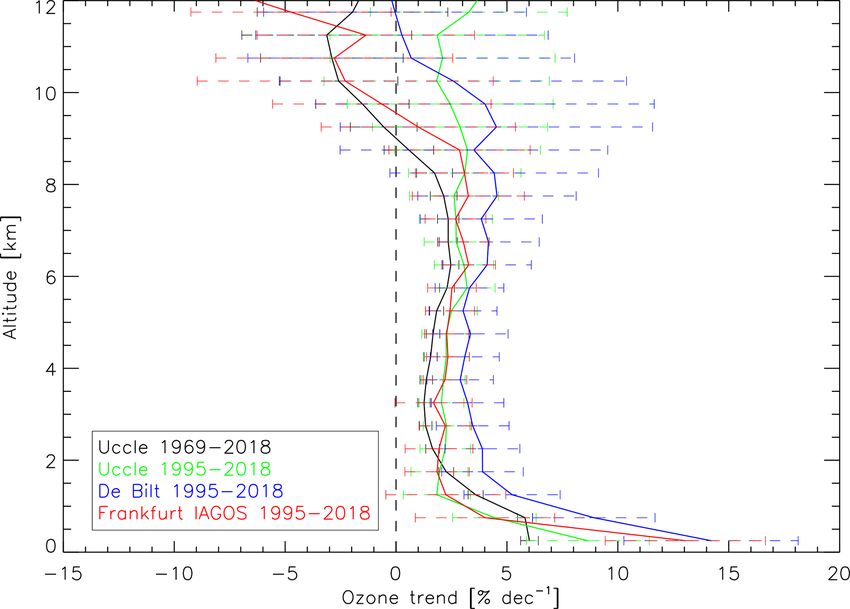
12390 R. Van Malderen et al.: Fifty years of balloon-borne ozone profile measurements at Uccle, Belgium
variability of the ozone measurements at Uccle is, therefore, the sensitivity of the estimated trends on the chosen (M)LR
organized into different sections. We first describe the strato- model is rather limited for the Uccle time series.
spheric (Sect. 4.1) and tropospheric (Sect. 4.2) ozone trends. The vertical profile of stratospheric ozone trends is shown
The relation to other co-located ozone measurements is de- in Fig. 2. From 1969 to 1997, stratospheric ozone concentra-
scribed in the appendices. Total ozone trends are treated in tions decrease almost uniformly (and significantly) at a rate
Appendix A, and the temporal behaviour of surface ozone of around −4 % per decade, except at the layers just above
and several ozone-depleting substances is discussed in Ap- the tropopause. Since 2000, the stratospheric ozone concen-
pendix B. trations have increased by about +2 % per decade but only
significantly at the layers below and at the ozone maximum
4.1 Stratospheric ozone trends (from 6 to 13 km above the tropopause, or 17 to 24 km for
an average tropopause height of 11 km at Uccle). The in-
To calculate the vertical distribution of trends in the strato- significant negative trend in the Uccle ozone concentrations
spheric ozone concentrations from the Uccle ozonesonde at the upper levels of Fig. 2 should be treated with caution,
data, we use the altitude relative to the tropopause height as the reliability of the ozonesonde instrument at those levels
as the vertical coordinate. The tropopause applied here is (above 30 km) is reduced. This is due to the increasing un-
the standard (first) thermal tropopause (WMO, 1957) and is certainty in the pump efficiency at low pressures, the differ-
derived from the vertical temperature profiles measured by ent stoichiometry of the chemical reaction due to a reduced
the Uccle radiosondes, as described in Van Malderen and amount of sensing solutions by evaporation, and frozen so-
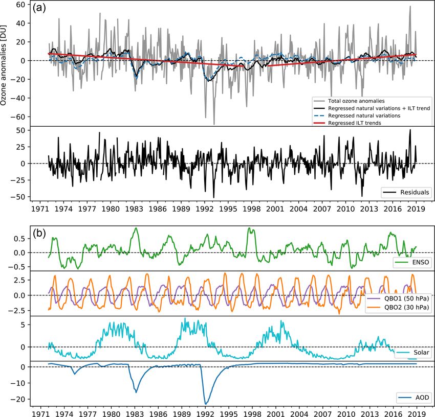
De Backer (2010). The implemented statistical model to cal- lutions. Additionally, an increase in the burst altitude in the
culate trends is the Long-term Ozone Trends and Uncer- Uccle ozonesonde time series in recent years and inhomo-
tainties in the Stratosphere (LOTUS) multiple linear regres- geneities due to changing pressure sensors with different ra-
sion (MLR) model (SPARC/IO3C/GAW, 2019). This model diosonde types might have had an impact on the ozone trends
uses an independent linear trend (ILT) method as trend term, at these very low pressures. In fact, the negative ozone trends
which is based on two different, independent, trends to de- are also less pronounced if calculated for absolute altitude
scribe the ozone decrease until 1997 (ODS increase) and levels. However, for these altitudes, we also prefer to cal-
the slow ozone increase since the early 2000s (after the culate the vertical ozone trends in altitudes relative to the
turnaround in ODS concentrations). These two periods have tropopause in order to cancel out the seasonal variation of the
been used since WMO (2014), and their use avoids end-point ozone peak altitude, which roughly follows the tropopause
anomalies near the turnaround in 1997 for the two indepen- height variation at Uccle: the ozone maximum peak is at its
dent linear trend terms in the ILT method. Additionally, the highest altitudes in summer (when the tropopause is also lo-
LOTUS regression includes two orthogonal components of cated higher) and is located at lower altitudes in winter (with
the Quasi-biennial Oscillation (QBO), the 10.7 cm solar ra- the lowest tropopause). This approach generally gives ver-
dio flux, the El Niño–Southern Oscillation (ENSO) without tical ozone trends that vary less over the different altitude
any lag applied, and the aerosol optical depth (AOD, ex- levels. When we compare the post-2000 trends with those
tended past 2012 by repeating the final available value from from the ozonesondes launched at De Bilt, the overall strato-
2012 as the background AOD, which should be a valid as- spheric positive insignificant trends apply for both stations,
sumption for Uccle). Four Fourier components represent- also at the higher altitude levels at De Bilt. The larger trend
ing the seasonal cycle are also included, unless (relative) uncertainties for the De Bilt time series can be explained by
monthly anomaly series are used as input ozone data. The the lower frequency of launches (once a week versus three
output of the LOTUS MLR model and the different contribut- times a week at Uccle). The statistically insignificant offset
ing terms (or proxies) for the monthly anomaly ozone con- between the Uccle and De Bilt trend estimates depends on the
centrations at the layer 10 km above the tropopause (close correction methods used at both sites, but differences in the
to the ozone peak) are shown in Fig. S5. The final choice vertical ozone distribution (up to 5 % in the stratosphere), of
of those proxies (and possible lags) in LOTUS was based both geophysical and instrumental origin, also have an im-
on retaining the optimal regression for the global analysis pact on the trend values (see e.g. Figs. 10a and 12 in Van
of satellite data and broad latitude band analyses. There- Malderen et al., 2016, in which a more detailed explanation
fore, proxies describing rather local or small-scale phenom- of the differences in vertical ozone distribution and trends
ena might not have been included in the general “LOTUS re- between Uccle and De Bilt is given).
gression” model. In particular, using an alternative stepwise The lower stratospheric ozone trends deserve more discus-
multiple linear regression model for the Uccle stratospheric sion here, as Ball et al. (2018, 2019) reported a significant
ozone amounts, we found that the Uccle tropopause pres- decline in lower stratospheric (13–24 km) ozone amounts
sure and the Arctic Oscillation are significant proxies as well for the respective 1998–2016 and 1998–2018 periods from
(contributing statistically significant, i.e. at the 95 % signifi- multiple (merged) satellite measurements in the lower strato-
cance level of the t test, to the regression coefficient). How- sphere between 60◦ N and 60◦ S. Moreover, the latest Scien-
ever, here, the analysis is limited to the LOTUS model, and tific Assessment of Ozone Depletion (WMO, 2018), largely
Atmos. Chem. Phys., 21, 12385–12411, 2021 https://doi.org/10.5194/acp-21-12385-2021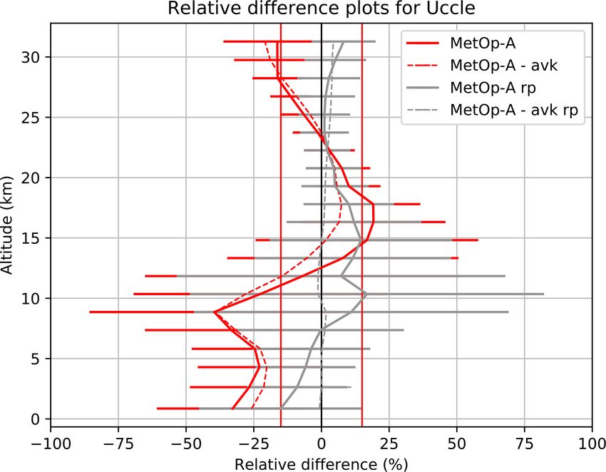
R. Van Malderen et al.: Fifty years of balloon-borne ozone profile measurements at Uccle, Belgium                                12391

                                                                        significant, we found that the positive Uccle ozone trends in
                                                                        the lower stratosphere are rather robust, independent of the
                                                                        starting date (1997/1998/2000), the vertical coordinate sys-
                                                                        tem used (absolute or relative to the tropopause), and the
                                                                        trend model used (LOTUS MLR or simple linear fit). The
                                                                        lower stratospheric ozone trends derived from the De Bilt
                                                                        time series show a larger variability between positive and
                                                                        negative statistically insignificant values, especially in the
                                                                        lowest 10 km.
                                                                           Ball et al. (2020) investigated if the aforementioned
                                                                        changes in ozone and transport are also found in other strato-
                                                                        spheric variables like the temperature. Globally, a reduction
                                                                        in lower stratospheric ozone should lead to reduced radiative
                                                                        heating and a decrease in observed temperature (see refer-
                                                                        ences in Ball et al., 2020). Quasi-global lower stratospheric
                                                                        temperatures from observations and in CCMs indeed de-
Figure 2. Vertical distribution of trends in stratospheric ozone        creased, with the post-2000 negative temperature trend being
concentrations at Uccle for different periods (see text) and at De      smaller compared with pre-1998, mimicking the observed
Bilt (2000–2018). The trends and their uncertainties are calculated     lower stratospheric ozone trends (Ball et al., 2020; but also
with the LOTUS multiple linear regression model (see text and           Maycock et al., 2018), although not the modelled ozone in-
SPARC/IO3C/GAW, 2019), including an independent linear trend            crease after 2000. On a smaller (European) scale, Philipona
term. The 2σ error bars represent the trend uncertainty estimated by    et al. (2018) found very similar seasonal and annual changes
the regression model (using the fit residuals). For the Uccle 1969–
                                                                        for temperature and ozone when averaging the Payerne, Ho-
2018 time series only, one linear trend term is included in the model
instead. The output of the LOTUS MLR model and the different
                                                                        henpeissenberg, and Uccle ozonesonde measurements. With
contributing terms for the monthly anomaly ozone concentrations         the exception of the fall season, annual and seasonal profiles
at the layer 10 km above the tropopause are shown in Fig. S5.           switch from negative to positive trends before and after the
                                                                        turn of the century for both ozone and temperature (see Fig. 4
                                                                        in Philipona et al., 2018). Here, on the local scale of Uccle
                                                                        and De Bilt, we also investigated the link between the lower
based on the LOTUS final report (SPARC/IO3C/GAW,                        stratospheric ozone and temperature trends (see Fig. S6). Be-
2019), concluded that “there is some evidence for a decrease            fore 1997, the entire stratosphere above Uccle cooled sig-
in lower stratospheric ozone from 2000 to 2016”, although               nificantly by −0.9 to −0.5 ◦ C per decade, in line with the
not statistically significant in most analyses. This decline,           decreasing stratospheric ozone concentrations. After 2000,
contradictory to the decline in ozone-depleting substances              the stratospheric cooling at both Uccle and De Bilt ceased at
since 1997, is surprising, and the current state-of-the-art             the altitudes where ozone concentrations peak (see Fig. S6)
chemistry climate models (CCMs) used in Ball et al. (2020)              and where their radiative impact on stratospheric tempera-
and Dietmüller et al. (2021) do not show a decrease but rather          tures is largest. Above and below the ozone maximum, the
an increase in the lower stratospheric mid-latitude ozone, al-          sign of the post-2000 temperature trends at Uccle (positive
though they confirm the lower stratospheric ozone decline in            and negative respectively) and De Bilt (negative and posi-
the tropics in the observations. Using the Modern-Era Ret-              tive respectively) are reversed. As such, there is no direct im-
rospective Analysis for Research and Applications Version 2             print of the slightly positive lower stratospheric ozone trends
(MERRA-2) ozone output fields, Wargan et al. (2018) found               since 2000 in the temperature variability, in particular for Uc-
a discernible negative trend of −1.67 ± 0.54 Dobson units               cle. However, this might not be expected on a local scale,
per decade in the 10 km layer above the tropopause between              and in addition to ozone, stratospheric temperatures are af-
20 and 60◦ N, and they attributed the trend to changes driven           fected by radiative effects from CO2 , N2 O, and CH4 as well
by dynamical variations (as in Chipperfield et al., 2018), in           as stratospheric water vapour and chemical changes in these
the form of enhanced isentropic mixing between the tropi-               gases (Ball et al., 2020). These authors point to the increas-
cal (20◦ S–20◦ N) and extratropical lower stratosphere over             ing stratospheric water vapour amounts in the CCMs since
the past 2 decades. In a follow-up study, Orbe et al. (2020)            1996 in the mid-latitudes, cooling the lower stratospheric, to
demonstrated that in the Northern Hemisphere (NH), this                 reconcile the increasing lower stratospheric ozone concentra-
mid-latitude ozone decrease is primarily associated with                tions in the models with their stratospheric cooling over the
changes in the advective circulation rather than changes in             same period and latitudes.
mixing. In this study, both the Uccle and De Bilt time se-                 Finally, as we use the altitude relative to the tropopause as
ries do not show a significant decline in lower stratospheric           vertical coordinate, we should also mention the time vari-
(13–24 km) ozone amounts. On the contrary, although never               ability of the tropopause height, which might impact the

https://doi.org/10.5194/acp-21-12385-2021                                             Atmos. Chem. Phys., 21, 12385–12411, 2021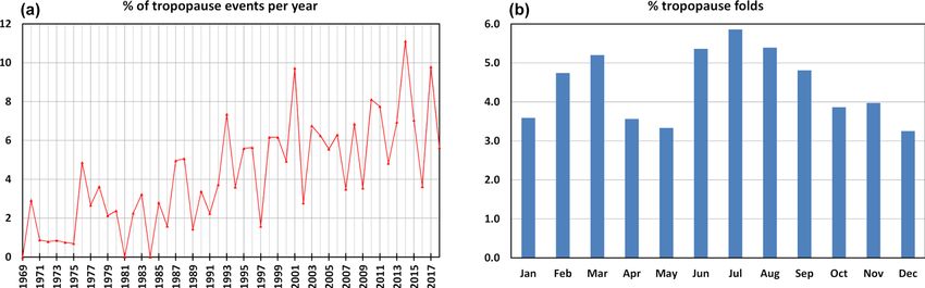
12392                 R. Van Malderen et al.: Fifty years of balloon-borne ozone profile measurements at Uccle, Belgium

lower stratospheric ozone trends. The tropopause height is              Here, we calculated the tropospheric ozone trends from the
increasing at both Uccle and De Bilt for all considered pe-         Uccle and De Bilt ozonesonde time series and the MOZAIC
riods, although with different magnitudes: for Uccle, these         (Measurement of Ozone and Water Vapour by Airbus in-
are 6.98 ± 1.12 m per decade (1969–2018), 13.81 ± 3.00 m            service Aircraft) and IAGOS (In-service Aircraft for a Global
per decade (1969–1996), and 11.62 ± 79.42 m per decade              Observing System) ascent and descent profiles at Frankfurt
(2000–2018), whereas for De Bilt the post-2000 trend mag-           airport, about 320 km from Uccle. This MOZAIC-IAGOS
nitude is 25.73 ± 19.23 m per decade. These increases in            dataset consists of more than 27 600 profiles, starting in Au-
tropopause altitudes are consistent with results from the           gust 1994, and is combined with the data from Munich air-
global study in Xian and Homeyer (2019) based on radioson-          port, approximately 300 km southeast of Frankfurt, between
des and reanalyses, although with smaller magnitudes (they          2002 and 2005 (about 4200 flights), to fill a large data gap
found increases of 40–120 m per decade for the 1981–2015            in 2005 (also done in e.g. Petetin et al., 2016). With typical
period). The thermal expansion of the troposphere and the as-       horizontal ozone correlation lengths of about 500 km in the
sociated increase in tropopause height have been proposed as        troposphere (Liu et al., 2013), some correlation of especially
robust fingerprints of anthropogenic climate change based on        free-tropospheric ozone trends between Uccle and Frankfurt
multiple pieces of observational and model evidence (Santer         and between Uccle and De Bilt is expected. We used sim-
et al., 2003; Seidel and Randel, 2006; Lorenz and DeWeaver,         ple linear trends based on the monthly anomalies at different
2007).                                                              altitude levels (see Fig. 3), as there is no consensus regard-
   We can conclude here that the Uccle stratospheric ozone          ing which proxies should be used to account for natural vari-
trends before 1997 are well understood but that the behaviour       ability. First, for the 1995–2018 period, the extremely good
after 2000 is harder to explain, especially for the lower strato-   agreement between the Uccle (in green in Fig. 3) and IA-
sphere, because of the lack of a clear link with stratospheric      GOS (in red) vertical ozone trends in the free troposphere (3–
temperature variability and the impact of the tropopause            8 km) is striking. Although the integrated tropospheric ozone
variability. The link between the Uccle stratospheric ozone         amounts for this altitude range are lower for the region above
trends and those from the total ozone column measured with          Frankfurt (14.9 DU) than above Uccle (16.2 DU), the over-
co-located spectrophotometers is discussed in Appendix A.           all relative trends are similar (2.09 ± 1.01 % per decade and
                                                                    2.47 ± 1.01 % per decade respectively; see Fig. S7). The De
4.2   Tropospheric ozone trends                                     Bilt trends (in blue in Fig. 3) are larger in the free troposphere
                                                                    and also have larger uncertainties due to the lower launch fre-
Ozone in the troposphere is affected by many processes.             quency. In this context, we mention the sensitivity analysis of
Stratosphere–troposphere inflow and photochemical forma-            IAGOS profiles above Europe by Chang et al. (2020), which
tion by interaction with sun light and ozone precursors (NOx ,      concluded that an optimal sample frequency of 14 profiles
CO, and volatile organic compounds) increase the ozone lev-         per month is required to calculate trends with their integrated
els, whereas photochemical destruction of ozone under low-          fit method (and about 18 profiles a month when this method
NOx conditions (e.g. marine boundary layer and free tropo-          is not used). Near the surface, the De Bilt trend is in bet-
sphere, via the OH–HO2 cycle) or at high NOx concentra-             ter agreement with the Frankfurt trend, but the local surface
tions (urban regions under titration, i.e. via reaction with NO)    ozone production and destruction and the boundary layer dy-
and dry deposition on the ground removes ozone from the             namics can vary substantially between the three sites consid-
troposphere. Its short lifetime causes highly variable ozone        ered here, so that the boundary ozone distribution and trends
concentrations in space and time, which complicates the un-         at the three sites are likely to be uncorrelated. However,
derstanding of the processes at play at all relevant spatio-        comparing the lower tropospheric IAGOS measurements at
temporal scales (Young et al., 2018). Moreover, the produc-         Frankfurt with nearby (within 50–80 km) and more distant
tion of ozone in the troposphere is sensitive to variations in      (within 500 km) surface stations, Petetin et al. (2018) showed
air temperature, radiation, and other climatic factors (Monks       that the IAGOS observations in the first few hundred metres
et al., 2015).                                                      above the surface at Frankfurt airport have a representative-
   Tropospheric ozone is measured with ozonesondes, by              ness typical of suburban background stations (such as Uccle
commercial aircraft, with different types of ground-based re-       and De Bilt), and as one moves higher in altitude, the IAGOS
mote sensing instruments, and with satellite instruments. Be-       observations shift towards a regional representativeness. A
sides clear regional differences, the distribution and trends       detailed description of the surface ozone trend at Uccle and
in ozone in the troposphere are not always consistent be-           its relation with ozone precursor trends is provided in Ap-
tween these different datasets or even not between differ-          pendix B.
ent retrieval methods of the same satellite (e.g. Cooper et             In the upper troposphere, the ozone concentration trends
al., 2014; Gaudel et al., 2018). In fact, measuring the ver-        deviate more between the different datasets, both in mag-
tical profile of tropospheric ozone concentrations from satel-      nitude and sign, with larger trend uncertainties. At these
lites remains very challenging and relies on ground-based re-       altitudes, the aircraft could be very distant from Frankfurt
trievals of ozone for validation (see Sect. 5).                     (or Munich) airport, as the ascent/descent profiles stop/start

Atmos. Chem. Phys., 21, 12385–12411, 2021                                            https://doi.org/10.5194/acp-21-12385-2021
R. Van Malderen et al.: Fifty years of balloon-borne ozone profile measurements at Uccle, Belgium 12393 Figure 3. Vertical distribution of trends in tropospheric ozone concentrations at Uccle for different periods, and at De Bilt (ozonesonde data) and Frankfurt (IAGOS data) for 1995–2018. Simple linear trends are calculated for monthly ozone anomalies in 1 km altitude ranges, and the error bars are 2σ standard deviations. The same colour coding is used as in Fig. 2: trends for the most recent Uccle sub-period (here 1995–2018) are in green; for the entire Uccle time series trends, we use black; and the De Bilt trends are shown in blue. The red line denotes the Frankfurt IAGOS trends in this figure. at about 400 to 500 km from the airport. Hence, the mea- sign of the ozone trends (Gaudel et al., 2018, and references surements at these altitudes represent large areas. Therefore, therein). However, Cooper et al. (2020) concluded, based the closer agreement between the Uccle and De Bilt trends on the IAGOS observations, that the western Europe free- above 8 km compared with the IAGOS trend might also be tropospheric trends since 1995 are predominantly positive. attributed to a similar source region. Moreover, at these alti- Using a different statistical approach, i.e. a nonlinear regres- tudes, the trends do not represent the tropospheric ozone tem- sion fit of a quadratic polynomial to normalized, deseason- poral variability only, as the mean tropopause height ranges alized monthly mean ozonesonde (merged data from Uccle, between 10.5 km (winter time) and 11.5 km (summer time), Hohenpeissenberg, and Payerne) and MOZAIC/IAGOS data with standard deviations between 1 and 1.5 km, at both Uc- (Frankfurt) between 3 and 4 km altitude, Parrish et al. (2020) cle and De Bilt. As a consequence, lower stratospheric ozone indicated that those ozone concentrations increased through concentrations will contribute to the estimated trends in the the 1990s, reached a maximum in the years 2001 (merged upper altitudinal levels of Fig. 3. ozonesonde) and 2007 (IAGOS), and have since decreased. The Uccle tropospheric ozone concentrations have been To explain the tropospheric ozone concentration trends, increasing at about the same rate since 1969 (in black in Griffiths et al. (2020) used a chemistry climate model em- Fig. 3) as they have since 1995 (in green in Fig. 3), and ploying a stratosphere–troposphere chemistry scheme and the post-2000 increase rate is also very similar (not shown found that, for the 1994–2010 period, despite a levelling-off here, but it is also suggested in the tropospheric ozone col- of emissions, increased stratosphere-to-troposphere transport umn time series shown in Fig. S7). The increase in (free) tro- of recovering stratospheric ozone drives a small increase in pospheric ozone concentrations above Uccle until the early the tropospheric ozone burden. Taking advantage of the high 2000s is consistent with the findings reported above (west- vertical resolution of the ozone profiles and the high fre- ern) Europe in the literature review of Cooper et al. (2014). quency of launches at Uccle, we focus on the time variability Over the 2000-2014 period, the emissions of the key ozone of specific cases of deep intrusions of stratospheric air into precursor, nitrogen oxides (NOx ), declined in North Amer- the troposphere (i.e. tropopause folds). Akritidis et al. (2019) ica and Europe due to transportation and energy transforma- stressed the role of tropopause folding in stratosphere-to- tion (Hoesly et al., 2018). Therefore, the overall increase in troposphere transport (STT) processes under a changing cli- ozone concentrations has flattened but has resulted in spa- mate, suggesting that tropopause folds will be associated tially and seasonally varying tropospheric ozone trends over with both the degree of ozone STT and inter-annual vari- North America and Europe, without consistency in even the ability in ozone STT. Tropopause folds occur because of https://doi.org/10.5194/acp-21-12385-2021 Atmos. Chem. Phys., 21, 12385–12411, 2021
12394                 R. Van Malderen et al.: Fifty years of balloon-borne ozone profile measurements at Uccle, Belgium

the ageostrophic circulation at the jet entrance and coincide     port of ozone from the stratosphere into the troposphere and,
with the frontal zone beneath the jet. The automatic algo-        hence, more tropopause folding events. Akritidis et al. (2019)
rithm applied in this work detects tropopause folds in the        elaborated that the degree of increase in the downward trans-
Uccle ozone-sounding profiles as ozone-rich (two criteria),       port of stratospheric ozone is partially driven by the long-
stable (one criterion), and dry (one criterion) air mass layers   term changes in tropopause fold activity.
located in an upper-level front in the vicinity of an upper-         To conclude, we found very consistent positive verti-
tropospheric jet stream (two criteria), and it is described in    cal tropospheric ozone trends between Uccle, De Bilt, and
Van Haver et al. (1996). This identification by means of the      Frankfurt (IAGOS) since 1995, which are consistent with
above-mentioned six criteria is also illustrated in an example    other studies, both observational studies and those using a
of an ozone sounding containing a tropopause fold in Fig. S8.     modelling approach, but different processing and statistical
   Tropopause folds are rather rare events at Uccle: out          methodologies can result in different European trend patterns
of the 6526 soundings analysed for the 50-year period             for the last 2 decades.
(1969–2018), only 290 soundings (or 4.4 %) showed evi-
dence of a tropopause folding. However, similar occurrence
rates (between 3 % and 10 %) have been found over Eu-             5     Validation of satellite ozone retrievals with Uccle
rope at French ozonesonde sites (Beekmann et al., 1997)                 ozonesonde data
and using other techniques (Rao et al., 2008; Antonescu
et al., 2013). On a monthly scale, most folding events oc-        Ozonesondes are virtually all-weather instruments (i.e. unaf-
cur in March, June, July, and August (occurrence > 5 %),          fected by clouds and precipitation) in contrast to most spec-
whereas in January, April, May, and December, the amount          troscopic techniques, and they provide high vertical resolu-
is lower (Fig. 4). Most important here within the context         tion ozone profiles from the ground to about 30 km. There-
of the tropospheric ozone trends is the dramatic increase         fore, satellite algorithms are based on ozonesonde clima-
in the amount of tropopause folding events over time with         tologies and, in turn, satellites are validated by the sondes.
a rate of 0.14 ± 0.02 % yr−1 (see also Fig. 4). Van Haver         Since the start of the ozone-measuring satellite era, ozone
et al. (1996) detected a smaller and insignificant trend of       profiles from soundings at Uccle have been used for the val-
0.07 ± 0.11 % yr−1 at Uccle for the 1969–1994 period. On          idation of satellite ozone retrievals, e.g. the Stratospheric
the one hand, the large increase over the entire time period      Aerosol and Gas Experiment (SAGE) II satellite profiles
might be explained by some technical aspects. Firstly, the        (Attmannspacher et al., 1989; De Muer et al., 1990). In this
higher vertical resolution of the sounding data in the more       section, we give some recent examples of the application of
recent digital era (since 1990) might have an impact on the       the Uccle ozone profile data for operational satellite vali-
larger detected number of tropopause folds (thinner layers        dation (Sect. 5.1) and for the scientific evaluation of both
might be detected), although the number of events has con-        stratospheric (Sect. 5.2) and tropospheric (Sect. 5.3) ozone
tinuously increased since then, at a slightly smaller annual      profile retrievals by satellite instruments. In these latter two
rate of 0.12 ± 0.05 %. Secondly, a visual inspection of all       sections, we also illustrate that a consistent and homogenous
profiles fulfilling at least five of the tropopause fold detec-   ozonesonde dataset, such as that from Uccle, is crucial to
tion criteria led to a higher number of (manually) identified     determine the long-term stability of (merged) satellite ozone
events (around 50 more), especially at the beginning of the       retrievals.
time series. This is explained by the fact that the low hu-
midity criterion was often not met in the automatic detection     5.1    Operational validation within EUMETSAT
because there were no humidity data or the humidity sensor               AC SAF
was iced (following the icing recognition algorithm of Leit-
erer et al., 2005). More recent types of radiosonde humid-        As partner of the European Organisation for the Exploita-
ity sensors (in use since 2007 at Uccle) prevent ice contam-      tion of Meteorological Satellites (EUMETSAT) Atmospheric
ination by heating the sensors during flight. However, this       Composition Satellite Application Facilities (AC SAF), RMI
manual (and hence more subjective) mode of the algorithm          is responsible for the validation of different ozone products
still gives a 0.09 ± 0.02 % annual increase in the frequency of   (ozone profiles and (tropical) tropospheric ozone columns;
tropopause fold events since 1969. Therefore, we believe that     see Hassinen et al., 2016; Valks et al., 2014; van Peet et
the significant increase, although possibly overestimated by      al., 2014) from the Global Ozone Monitoring Experiment-2
the automatic procedure, is nevertheless a robust feature of      (GOME-2) and Infrared Atmospheric Sounder Interferome-
the analysis. Additionally, a higher rate of tropopause fold-     ter (IASI) instruments on board the MetOp A, B, and C satel-
ing events is expected due to climate change (Tarasick et al.,    lite platforms. These different instruments give the opportu-
2019, and references therein): climate change is projected        nity to obtain a unique dataset, retrieved with an identical
to increase planetary wave activity inducing an accelerated       technique, from the beginning of the MetOp-A/GOME-2 in-
Brewer–Dobson circulation. This acceleration, along with          strument in 2007 until the phase-out of the third instrument
stratospheric ozone recovery, will lead to the increased trans-   (MetOp-C/GOME-2), which is officially foreseen in 2022.

Atmos. Chem. Phys., 21, 12385–12411, 2021                                          https://doi.org/10.5194/acp-21-12385-2021
R. Van Malderen et al.: Fifty years of balloon-borne ozone profile measurements at Uccle, Belgium                                  12395

Figure 4. (a) Relative frequency of detected tropopause folding events per year in the ozone soundings at Uccle. (b) Relative frequency of
tropopause folding events per month.

GOME-2 ozone profiles are given as partial ozone columns,              resolution will have the largest effect here by removing de-
expressed in Dobson units, on 40 varying pressure levels be-           tails of the differences. Secondly, as the GOME-2 ozone pro-
tween the surface level and 0.001 hPa and are calculated by            file product is based on UV measurements, it is sensitive to
the Ozone Profile Retrieval Algorithm (OPERA; van Peet et              degradation of the UV sensor (van Peet et al., 2014; Munro et
al., 2014). The a priori information used for the retrieval is         al., 2016). For example, the measured values of the GOME-
obtained from McPeters and Labow (2012).                               2A irradiance in the UV (below 300 nm) had decreased by
   For the validation of GOME-2 ozone profiles within the              roughly 80 % in 2016 (since its launch in 2007). As the verti-
AC SAF, ozonesonde measurements are extensively used.                  cal ozone profile retrieval algorithm depends on an absolute
However, for a meaningful comparison, the ozonesonde pro-              calibrated reflectance (sun-normalized radiance), there is a
files need to be integrated first between the GOME-2 pres-             need to correct for this temporal change of the (joint) radi-
sure levels. When comparing a single ozonesonde profile                ance and irradiance. This method depends on the assumption
with different GOME-2 profiles, the actual reference ozone             that, taken as an average across the globe, the atmospheric
values are not identical due to the fact that the GOME-2 ver-          constituents (mainly ozone) will be close to the multi-year
tical levels vary from one measurement to another. GOME-2              climatological value from McPeters and Labow (2012). The
has a nominal spatial resolution of 80 km × 40 km, but for the         climatological ozone profile is then scaled with the assimi-
shortest UV wavelengths, the integration time takes 8 times            lated total ozone columns to get the overall ozone absorp-
longer because of the lower number of photons arriving on              tion correct (Tuinder et al., 2019). This degradation correc-
the detector pixels. Furthermore, as the ozonesondes and the           tion has been applied to the data for the relative differences
satellite do not have the same vertical resolution, it is nec-         with the Uccle data in Fig. 5 (in grey). From this figure,
essary to consider the averaging kernels (AVK) in order to             it should be clear that this degradation correction signifi-
“smooth” the ozone soundings towards the resolution of the             cantly improves the agreement with the Uccle ozonesonde
satellite (Rodgers, 2000).                                             data compared with the operational product (in red), resulting
   In Fig. 5, the relative differences between the MetOp-A             in relative differences between GOME-2 ozone profiles and
operational ozone profile product and the Uccle ozonesonde             the Uccle data within the target error range of 15 % (marked
profiles are shown for the year 2018 (in red). The following           by the vertical red lines). The improvement after degradation
co-location criteria were applied: a geographic distance of            correction is a promising result, showing the challenge for
less than 100 km between the GOME-2 pixel centre and the               UV–VIS sounders to obtain a stable ozone profile product on
sounding station location, and a time difference of less than          different sensors (GOME-2A, 2B, and 2C) for different peri-
10 h between the pixel sensing and the sounding launch time.           ods using the same type of optical instrument. More feedback
The figure highlights two different aspects of the operational         on the status of the operational EUMETSAT product can be
validation. Firstly, it can be noted that applying the averag-         obtained in the validation reports, which are available on the
ing kernels to the sounding profiles improves the comparison           AC SAF website (https://acsaf.org, last access: 29 May 2020;
with the GOME-2 ozone product significantly (i.e. by 15 %),            e.g. Delcloo and Kreher, 2013).
in particular in the lower stratosphere (compare the full lines
with dashed lines in Fig. 5). The lower stratosphere is the
region with the highest ozone variability, so smoothing the
high-resolution ozonesonde profiles to the GOME-2 vertical

https://doi.org/10.5194/acp-21-12385-2021                                             Atmos. Chem. Phys., 21, 12385–12411, 2021
You can also read