Fips: an OpenGL based FITS viewer
←
→
Page content transcription
If your browser does not render page correctly, please read the page content below
Fips: an OpenGL based FITS viewer

                                                                   Matwey Kornilov, Konstantin Malanchev
                                                        Sternberg Astronomical Institute, Lomonosov Moscow State University
                                                                   Universitetsky pr. 13, Moscow 119234, Russia
arXiv:1901.10189v1 [astro-ph.IM] 29 Jan 2019

                                                              National Research University Higher School of Economics
                                                              21/4 Staraya Basmannaya Ulitsa, Moscow 105066, Russia

                                               Abstract
                                                FITS (Flexible Image Transport System) is a common format for astronomi-
                                               cal data storage. It was first standardised in the early 1980s [1]. Even though
                                               astronomical data is now processed mostly using software, visual data inspec-
                                               tion by a human is still important during equipment or software commissioning
                                               and while observing. We present Fips1 , a cross-platform FITS file viewer open
                                               source software [2]. To the best of our knowledge, it is for the first time that
                                               the image rendering algorithms are implemented mostly on GPU (graphics pro-
                                               cessing unit). We show that it is possible to implement a fully-capable FITS
                                               viewer using OpenGL [3] interface. We also emphasise the advantages of using
                                               GPUs for efficient image handling.
                                               Keywords: techniques: image processing, image-based rendering, graphical
                                               user interfaces

                                               1. Introduction

                                                    FITS (Flexible Image Transport System), a famous image format, was first
                                               introduced a few decades ago, in the early 1980s [1]. Since that time, it has
                                               become the most popular format to store astronomical optical observations.
                                               Now, in 2019, FITS looks like a legacy format rather than a modern tech-
                                               nology item [4]. For instance, it uses the big-endian storage format, while
                                               most current server, desktop and mobile processors use little-endian storage
                                               format [5, 6, 7]; moreover, FITS relies internally on a 2880-byte-alignment struc-
                                               ture [1]. Whereas it was a natural choice for tape-based storage media, modern
                                               file systems on hard drives and solid state drives operate with pages of 2N size.
                                               For some upcoming projects, it is the JPEG 2000 [8] data format that is being
                                               discussed now by the astronomical community [9].

                                                 ∗ Corresponding author
                                                   Email address: matwey@sai.msu.ru (Matwey Kornilov)
                                                 1 https://fips.space

                                               Preprint submitted to Astronomy and Computing                        January 30, 2019
However, there are two main things that make us believe that FITS will
continue be used for decades to come. First, bulk of astronomical data in the
world is stored in FITS format. Second, astronomical data acquisition software
or data processing software are mostly FITS-centric. As long as visual human
inspection of raw or processed astronomical image data is still an important part
in algorithm and software troubleshooting procedures, as well as in hardware
alignment and commissioning, it would be helpful to have yet another FITS
image viewer software.
There is, of course, a lot of available software doing this work well, among
them SAO DS9 [10], Ginga [11, 12], etc. All these solve the same problems while
rendering data from a file to the user screen. An application has to parse and
read the data from the file. Then, it has to make geometric transformations for
scale, pan, rotation, etc. After that, colour maps are applied in order to narrow
down the FITS range of values to the 8 bit colour depth.
In this paper we concentrate on how these tasks may be offloaded to the
GPU (graphics processing unit). Modern GPUs have many hard-wired features
accelerating typical 2D and 3D-rendering tasks. These advantages are employed
by a wide variety of desktop applications such as web-browsers [13, 14] and
even graphical terminal emulators [15, 16]. We propose a FITS viewer software
implementation based on the GPU acceleration. After a raw FITS file data
loaded into the GPU memory, the geometric and colour transformations are
handled by GPU.
It is widely believed by the developer community that software generally
should use a minimal amount of the computational resources while keeping its
source code simple, clear, and easily maintainable.2 The GPU-based end-to-end
rendering of the raw FITS file data fulfils both of this conditions. The specific
dedicated design of modern GPUs provides an opportunity to render graphics
in energy and computationally efficient way. GPU programming interfaces such
as OpenGL, Direct X, or Vulkan allow a programmer to describe the high-level
geometric and colour characteristics of the scene. In our case, only a few lines
of high-level source code are required to program GPU.
In this paper we prove that the end-to-end OpenGL rendering of FITS file
data can be practically implemented as software application. This proof of
concept application is called Fips. It is a cross-platform open-source graphical
user interface software. The application main window is shown in Fig. 1.
The outline of the paper is as follows. Section 2 explains briefly how modern
graphics processing units operate and how one could control them using the
OpenGL interface. Section 3 describes the essence of the FITS format and
2 Many recognised experts in computer science often note this. For instance, Cormen et al.
([17], § I.2) say: “If computers were infinitely fast, any correct method for solving a problem
would do. You would probably want your implementation to be within the bounds of good
software engineering practice...”; or Knuth ([18], § 1.1) says: “In practice we not only want
algorithms, we want good algorithms in some loosely-defined aesthetic sense. One criterion
of goodness is the length of time taken to perform the algorithm... Other criteria are the
adaptability of the algorithm to computers, its simplicity and elegance, etc.”.
2Figure 1: Fips interface on the macOS operating system. The user interface looks the same
both on Linux and Windows. A M31 galaxy image obtained by the MASTER robotic tele-
scopes network [19] is shown here.
how it can interoperate with the OpenGL. Then, in Section 4, we demonstrate
how the FITS data may be transformed into a coloured image displayed by
Fips. The software evaluation and testing are described in Section 5. In the
Discussion section, we highlight further possible applications of the techniques
described here. Finally, we summarise the advantages of the GPU use in the
Conclusion. Appendix A describes how the FITS and OpenGL coordinate
systems are connected to each other.
2. Brief Introduction to OpenGL
General-purpose graphics processing units are widely used in modern astron-
omy for solving visualisation problems [20] and computational linear algebra
problems [21, 22], with the latter seemingly more widespread. Thus, it makes
sense to briefly introduce the graphics pipeline here. A more comprehensive
OpenGL description can be found in its specification [3]. In what follows, only
details that are important for current work will be highlighted.
OpenGL is essentially a programming interface, i.e. a library with a stan-
dardised set of functions available on different platforms or operating systems.
It is assumed (although not required) that the library functions should be imple-
mented using the graphics processing unit hardware, which is capable to perform
a limited set of the most frequently required graphics rendering operations.
Generally, the programming work that uses the GPU with OpenGL does
not resemble conventional programming; instead, one may substitute routines
3of some kinds into the predefined data processing pipeline and operate with the
predefined types of data objects.
In an OpenGL application, different kinds of objects may exist. A point in
3D space that belongs to a geometric object is called a vertex. In typical 3D
applications, geometric objects normally consist of hundreds and thousands of
vertices; however, for our purposes, it is sufficient to have four vertices forming
a rectangular plane in our application. The plane is used to draw picture on its
surface. Arrays of vertex attributes (coordinates) are transferred from CPU to
GPU.
It is usually convenient to define vertex coordinates in an object-centric co-
ordinate system. However we need to place each object at its desired place in
order to form the world scene. This is the reason for vertex shaders. These are
GPU-side routines (functions) performing an arbitrary geometric transforma-
tion of vertex coordinates. The shaders are designed to process only one vertex
at a time. Since there is no concurrence that allows engaging in parallel as many
shader units during the execution as are available at one particular hardware.
They are usually used to transform vertex coordinates from the local object co-
ordinate system to the camera coordinate system. The transformation is often
defined as a matrix-vector operation; these transformations may be of various
kinds: we can translate, rotate, scale or distort an object. In fact, what the user
can see at the display is a world projection onto the xy coordinate plane.
Graphical memory fragments that contain raster pictures are called textures.
They are similar to traditional uncompressed bitmap images and FITS images.
The texture content also may be transferred between CPU and GPU in both
directions. The possible ways to arrange the pixel colours in texture memory
are given in the OpenGL specification [3]. For instance, one may store a colour
picture as an array of usual RGB triplets and a monochromatic image as an
array of single channel pixels. The process of transforming FITS images into
OpenGL for all possible formats will be discussed in Section 4.
Texture data are accessed via samplers. A sampler can be thought of as the
C operator [] indexed by a real value coordinate rather than by an integer
index. Among other things, samplers perform the interpolation before returning
a value. There may be two kinds of interpolation: the nearest neighbour inter-
polation and the linear interpolation. Although we use the nearest neighbour
interpolation, the returned result is always normalised to [0; 1] range indepen-
dently of the data storage format.3 For instance, the standard 8-bit colour
channel value 255 stored in a texture will be returned as 1.0 by a sampler.
Vertices form the edges and faces of geometric objects, and textures can be
drawn on these faces. At the same time, the orientation between the surface and
the camera is also taken into account; for instance, the hidden parts of objects
are not rendered at all.
Fragment shaders are GPU routines that are used to colourise sides of ge-
3 OpenGL 3.0 and later versions support the access to an normalised raw value. As we see
later in Section 4, this does not give us a great advantage
4ometric objects. Formally, this can be considered as the mapping between
fragment coordinates and their required colour, where each fragment is a tiny
piece of the scene seen by the user. In our simple case, the fragment shader
prescribes that the hardware would draw the texture containing the image onto
a singleton rectangular plane without distortion.
After everything is loaded to the graphics memory and preconfigured, an
application would trigger the drawing, and the user would be able to see 3D
scene snapshot at the screen. In case the objects are to be rearranged, altered
vertex shaders parameters are loaded and the drawing is performed again. In
modern 3D professional software and games, it is usually required to perform
multiple renderings to achieve realistic light distribution over the single frame.
For this purpose, depth textures and stencils are used.
3. FITS Rendering Implementation
Our goal could be achieved by performing two tasks. First, we need to load
a FITS image to the graphics memory. Second, we should render the image
using the required orientation, magnification, colour-mapping, etc.
If any transformation between the FITS image memory representation and
GPU texture representation is needed, it would use additional CPU-based cal-
culations. This is why we focus on cases where byte-representations are similar
at CPU (FITS) and GPU (texture) sides. For instance, a 16-bit FITS image is
an array of subsequent 16-bit integers. A monochrome 16-bit texture is also an
array of subsequent 16-bit integers. Since it is monochrome (i.e. single-channel),
a single integer represents a whole single pixel. This means that memory repre-
sentations of the 16-bit FITS image and the 16-bit single channel texture should
be identical except for the byte order (see below). Unfortunately, this is not al-
ways the case. For instance, if we have a 64-bit integer FITS image, we cannot
just specify that the texture should have a single 64-bit channel, because there
are no 64-bit integer textures in OpenGL [3]. To overcome this difficulty, we
just set the OpenGL texture format for the image memory so that it still has
64-bit per pixel and, at the same time, multiple colour channels (for instance,
16-bit RGBA). This approach hinders, to some extent, the data access by GPU,
but we will show how to deinterleave colour channels to obtain the initial value
in Section 4.
Note, that the endianness is also accounted by OpenGL. FITS stores its data
in 8-bit bytes using the big-endian format [23]. On the other hand, OpenGL
uses the machine-specific byte ordering [3]. Today, the vast majority of work-
stations use the little-endian format, e.g. x86/x86-64 [5], ARM machines with
Windows [6], iOS [7], and almost all Linux-based operating systems with very
few exceptions. Fortunately, we do not need to explicitly handle the FITS en-
dianness. It is sufficient to specify that the data are big-endian on CPU when
calling the OpenGL data transport function. Although it is not strictly speci-
fied, the byte swapping may be even performed in the graphics processing unit
hardware if this is required while texture storing.
5(k − 1)-th pixel k-th pixel (k + 1)-th pixel
FITS data 01 ab 90 7d 60 95 40 00 01 64 92 37 36 7b 68 a0 01 82 fd f1 55 78 c9 00
Texture ab 01 7d 90 95 60 00 40 64 01 37 92 7b 36 a0 68 82 01 f1 fd 78 55 00 c9
Red Green Blue Alpha
6.515 · 10−3 5.432 · 10−3 5.889 · 10−3
Sampler output 5.644 · 10−1 5.711 · 10−1 9.919 · 10−1
3.772 · 10−1 2.128 · 10−1 3.338 · 10−1
2.500 · 10−1 4.087 · 10−1 7.851 · 10−1
Figure 2: Memory layout example. At the top layer, FITS image linear memory data represent
64-bit integer pixels in big-endian order. At the middle layer, the texture memory representa-
tion for a 16-bit RGBA (Red, Green, Blue, Alpha) pixel in little-endian architecture is given.
At the bottom layer, floating point vectors are shown that are returned by the sampler when
the texture is accessed.
Since the GPU has an access to the FITS data, the image can be easily
transformed and rendered. Note also that the following two tasks are com-
pletely separated when programming OpenGL. The first task is the geometric
transformation of 3D space objects. Assume that we have a rectangular plane
has the same aspect ratio as the initial FITS image has. A broad variety of ge-
ometric transformations may be applied to the plane independently of what is
going to be drawn on this plane. This is how the pan, scale and rotation are im-
plemented. One only needs to carefully program straightforward transformation
formulae given in Appendix A.
The second task is rendering the texture onto the plane. This is always
performed in the local plane coordinates independently of the final plane ori-
entation and the scale. The task that is handled in the fragment shader is
essentially the mapping between a local plane coordinate and its visible colour.
Specific coordinates are implicitly determined by OpenGL and the colours are
evaluated simultaneously.
4. Fragment Shader Organisation
The fragment shader is a place where colour transformations are performed.
Let us describe the tasks to be solved in the shader code:
• FITS format requires the following transformation to be applied to the
data stored in the file:
physical value = BSCALE · array value + BZERO, (1)
where BZERO and BSCALE are stored in the FITS header, physical value
is a ‘true’ value, and array value is a byte-representation stored in the
file. Since we load the whole file into the graphics memory, we have to
handle this equation using the GPU as well.
• Astronomical data usually have a greater number of bits per colour than
modern screens have or human eye can distinguish. In common modern
6operating systems, 8-bit colours are used, whereas astronomical data com-
ing from CCD are likely to contain 16-bit (or even greater) ones. This is
why we prefer to adjust minimal and maximal levels to give an image more
contrast in order to see all interesting details.
• Different colour mapping schemes should be applied to data. In FITS files,
we usually have single-channel colour formats. Each pixel is described by
a single value. In optical astronomy, it is usually expressed in ADU units
(analogue-digital units) coming from a CCD (charge-coupled device). [24]
So it is natural to represent the data as greyscale pixels. However, we
could use any other colour instead of white to represent the brightest
image pixels.
• The last but not the least is format converting. FITS supports different
data storage bit depths specified by the BITPIX header value: up to 64-bit
integer and floating point numbers.4 The challenge here is that earlier
OpenGL versions allow using only 8 or 16 bits per colour channel, and
even the latest OpenGL does not support 64-bit textures.
To solve this last task, we use the process of deinterleaving colours. First,
we are going to describe how the data are transformed in a forward way in the
example shown in Fig. 2. After that, we will construct the inverse transforma-
tion. At the top level of Fig. 2, three consecutive pixels of a 64-bit FITS image
are shown. The middle level presents the same data loaded into the little-endian
GPU. Since there is no option to specify its real 64-bit format in OpenGL, the
pixel is considered to have four subsequent 16-bit channels. The bottom level
displays what we may obtain when accessing the texture by the sampler. These
are four floating point numbers to represent a pair of bytes each. To summarise,
each texture pixel for the i-th colour channel (ti ) may be expressed as follows:
(n)
{y}i
N
ti = n , i = 0... −1 , (2)
2 −1 n
where y is the initial value; N is the real bit size of the input FITS pixel (64 in Fig. 2);
(n)
n is the bit size of the colour channel (16 in Fig. 2); {·}i denotes the i-th n-bit
word of · value (the i-th colour channel in Fig. 2); i = 0 corresponds to the
most significant word. Since the sampler returns the normalised value, we have
2n − 1 in the denominator, while ti ∈ [0; 1]. Note that Eq. (2) is still valid when
N = n and no colour transformation is performed.
The expression for the array value y may be written as follows:
N
−1
n
X
y= 2N −(i+1)n (2n − 1) · ti . (3)
i=0
4 The following FITS data formats exist: 8-bit unsigned integers (BITPIX = 8), 16-, 32-,
64-bit signed integers (BITPIX = 16, 32, 64), single and double precision floating point numbers
(BITPIX = −32, −64).
7Since the internal texture representation is unsigned, the following substitution
should be done for the signed integer (BITPIX = 16, 32, 64):
2n 1
t0 ← t0 − if t0 > . (4)
2n − 1 2
Using Eq. (1) and the linear normalisation transformation, we obtain the
following expression:
N
−1
BSCALE nX N −(i+1)n n BZERO − m
g= 2 (2 − 1) · ti + , (5)
M − m i=0 M −m
where m and M are the minimal and maximal physical values set by user,
respectively, according to Eq. (1). If a physical value ∈ [m; M ], then g ∈ [0; 1],
otherwise g is clamped to this interval.
Equation (5) may be rewritten in the following convenient inner product
form:
g = (c, t − z) , (6)
where t is the vector of ti values, c and z are vector functions of BSCALE, BZERO,
m, and M . The vectors c and z are constant for every image pixel, so they can
be precalculated on the CPU. OpenGL allows us to efficiently calculate inner
products on the GPU. Note that by construction, |zi | < 1 for every i, what
ensures that the precision is not lost in numerical operations.
The final fragment colour is the f vector consisting of four normalised com-
ponents: red, green, blue, and alpha. To represent the data in user colours, we
may calculate the fragment colour as follows:
f = (1 − g) f0 + gf1 , (7)
since g is implicitly clamped to the [0; 1] interval after using Eq. (6). This linear
interpolation is implicitly performed by the sampler of special one-dimensional
texture consisting of two-colour pixels (the interpolation node) that store the f0
and f1 colour constants. Further generalisation may be achieved if additional
interpolation nodes are added to the colour map texture, allowing an easy im-
plementation of multi-colour maps such as ‘black–blue–yellow‘.
In Table 1 we present particular values for n in different possible cases.
Note that the following equation should be used instead of (5) for floating point
formats:
BSCALE BZERO − m
g= y+ , (8)
M −m M −m
because the sampler output y is not normalised for floating point textures, and
the colour trick is not used in this specific case of floating point number represen-
tation in memory. In order to handle double precision floating point FITS files,
ARB gpu shader fp64 extension should be used [25]. In this case the internal
representation of GPU data is set up to two-channel 32-bit unsigned integers.
After that, the sampler output in the fragment shader is subjected to the action
of a specific built-in magic function. The function performs reinterpretation
cast, taking a pair of 32-bit unsigned integers obtained from the texture, and
returns the double precision floating point value.
8FITS BITPIX OpenGL 2.1 OpenGL 3
8 n = 8 (native) n = 8 (native)
16 n = 8 (Luminance, Alpha) n = 16 (native)
32 n = 8 (RGBA) n = 16 (Red, Green)
64 n = 16 (RGBA) n = 16 (RGBA)
−32 not supported† native
−64 not supported native via the extension∗
Table 1: Support matrix. Here, the specific values of n from Eq. (2) are presented for dif-
ferent possible cases. N = BITPIX for integer formats, negative BITPIX denotes floating point
numbers. The case n = N , when no colour trick is used, is denoted as ‘native’.
† single precision floating point textures are supported in OpenGL 2.1 via extensions but can-
not be used in Fips due to Qt framework limitations.
∗ double precision floating point values must be unpacked from two 32-bit unsigned integers
using ARB gpu shader fp64 extension.
16 2.5
Intel, 4096 × 4096 NVidia, 4096 × 4096
14 Intel, 800 × 448 NVidia, 800 × 448
2.0
12
Render time, ms
Render time, ms
10
1.5
8
1.0
6
4
0.5
2
0 0.0
8 16 32 -32 64 -64 8 16 32 -32 64 -64
FITS BITPIX FITS BITPIX
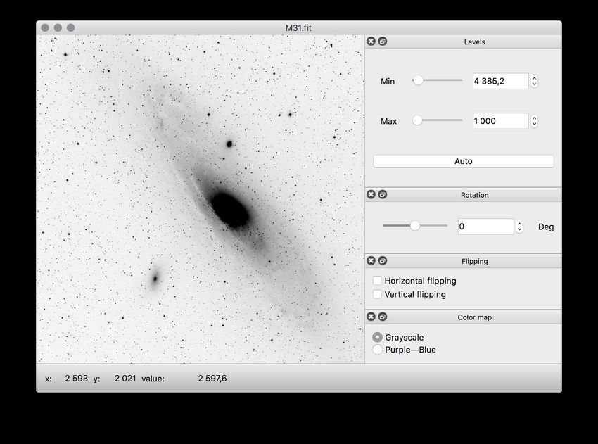
Figure 3: Box-and-whisker plots for rendering time at Intel HD Graphics 4000 (left panel)
and NVidia GeForce GT 635M (right panel). The boxes show the quartiles. The ends of the
whiskers represent the lowest and the highest result still within 1.5 interquartile range.
45
llvmpipe, 4096 × 4096 llvmpipe, 800 × 448
40 Intel, 4096 × 4096 Intel, 800 × 448
NVidia, 4096 × 4096 NVidia, 800 × 448
35
30
Render time, ms
25
20
15
10
5
0
8 16 32 -32 64 -64
FITS BITPIX
Figure 4: Box-and-whisker plot for rendering time at Mesa llvmpipe software renderer. The
notation is the same as for Fig 3. Median rendering times for Intel and NVidia are shown for
comparison.
95. Software Evaluation and Validation
Users expect modern applications to provide responsive user interface. In-
terface responsiveness gives a user ability to immediately see the results of user
actions. For instance, it is important when touch-pad gestures are employed
as a part of user interface requiring continuous user actions to be handled with
low possible latency. In our case the following user actions trigger the image
redrawing: changing the cut levels, switching colour maps, zooming, panning,
and rotating the image. We measured the time required to redraw the image
under these typical actions.
Three hardware setups have been tested with the laptop PC. The software
rendering was performed using Mesa llvmpipe5 driver with Intel Core i7-3520M
CPU, the hardware rendering was performed using integrated Intel HD Graph-
ics 4000, and the hardware rendering was performed using discrete NVidia
GeForce GT 635M. We considered two image geometry sizes: 800 × 448 pix-
els and 4096 × 4096 pixels, with all six bit depths, twelve image files in total.
In all cases the application ran in full screen mode at 1980 × 1080 resolution.
This allowed us to examine two cases: when the image was stretched for the
small images and shrunk for the large images. For each case, a few hundreds of
drawings were carried out.
We found that the image rotation rendering is the most expensive of all
operations, so expenses for it may be considered as an upper bound estimate
compared to other expenses. The obtained results are given in Fig. 3 and Fig. 4.
The following specific features can be seen in the figures. One may see that
Intel hardware behaves similarly to NVidia hardware. Note that the required
memory size is proportional to the image bit depth. In Fig. 3, one can see that
the rendering time for the 4096 × 4096 pixels image depends almost linearly
on the bit depth. In this case, the performance seems to be limited mainly by
the memory bandwidth. At the same time, the 800 × 448 pixels image is small
enough to fit into modern memory caches and therefore no dependence on the
bit depth is revealed in all these three rendering engines. Also in the case when
the double precision floating point image is formed on the NVidia GPU, some
specific additional overheads appear.
The same kind of measurements were carried out for panning. We found that
the rendering time doesn’t depend on the image bit depth. It is approximately
the same as the time for rotating the 8-bit image. It seems that the time depends
only on the visible image size.
The llvmpipe renderer is considerably slower as compared to the hardware
cases. Note that the llvmpipe produces just-in-time compiled code highly op-
timised for using CPU vector instructions. Hence, the llvmpipe rendering time
is considered as a lower bound estimate for any CPU-based implementation.
However, we were able to see some glitches during llvmpipe rendering for all
considered actions. The glitches look like vertical synchronisation issues: the
5 https://www.mesa3d.org/llvmpipe.html
10top and bottom parts of the picture correspond to the different subsequent
frames. This is in agreement with Fig. 4. Indeed, it may take more than 30 ms
to render the 4096 × 4096 pixels image which corresponds to ≈ 30 frames per
second, given that the measurements were carried out on an unloaded CPU.
The measuring data strongly indicate that the GPU-based implementation is
more efficient.
Functional testing of the graphic user interface application is a more chal-
lenging task than to test the server application. This is explained by the fact
that automatic unit tests cannot be applied to the application graphic interface
parts. Therefore, we use the unit testing where it is possible, such as parsing
the FITS files, or assessing the coefficients in Eq. (6). The integration of Travis
CI and GitHub allows us to easily check the application for a wide range of
compilers and Qt framework versions.
To ensure validity of the algorithm described in Section 4, we may either
render the image to a texture framebuffer, extracting pixel numeric values, or
we may use the system colour picker application to see pixel values on the screen.
We used the latter approach since our key interest is to find out what the user
can actually see on the screen. A simple greyscale gradient testing image allows
us to perform this kind of end-to-end manual testing.
6. Discussion
The OpenGL application may be helpful for astronomical purposes not only
due to its ability to perform simple FITS image rendering. The so-called texture
arrays available with OpenGL 3 may be properly used to support 3D FITS data.
A 3D data cube stored in GPU video memory in the form of texture array
representation may give us an opportunity to implement efficient GPU video
playback. The representation of data cubes in the form of a video is currently
implemented in e.g. Ginga and FITSWebQL FITS viewers [11, 26].
Since OpenGL is capable to support the opacity, we may use another in-
teresting option; namely, to draw multiple FITS images as semi-transparent
colour layers, differently placed and differently orientated. This option would
be helpful for applications similar to those in which the blinking technique in
astronomy is currently used: the manual transient object search. A similar
technique is widely adopted by amateur astronomers [27, 28]. However, in this
case, a nonlinear geometric transformation of the image is ordinarily required
to compensate for third order aberrations. This may be easily done using the
expansion of a current four-vertex-rectangle plane to a triangle mesh, a common
technique employed in the 3D computing world.
Note also that embedding such a geometric transformation engine into the
astronomical image processing pipeline considerably increases the processing
rate. This property is very valuable when looking for asteroids using robotic
observatories. The technology incorporating OpenGL into the head-less server
application is called EGL (Embedded GL); it uses a texture attached to a frame
buffer object instead of the hardware display that performs scene rendering [29].
11Thus, the rendering output may be downloaded to the CPU after the render
operation is performed.
One challenge for upcoming extra-large survey projects, such as LSST [30],
is to increase the astronomical image processing cadence. When using OpenGL
computing shaders (available with OpenGL 4.3) or OpenCL/OpenGL integra-
tion, a full stack of the common astronomical pipeline may be implemented:
from bias subtraction and flat fielding to pixel clustering for star extraction, as
it has been proposed e.g. by Warner, et al. [31].
Many of the techniques we have described could be applied to WebGL-based
FITS image rendering [32]. WebGL is a standard programming interface for
modern web browsers that allows OpenGL programming in JavaScript. Sev-
eral years ago, there was some publication of plans for the implementation of
telescope control system interfaces and astronomical data archives in the form
of web applications. This approach has many advantages. For example, web
applications scale well for any OS and any platform, they do not require in-
stallation and may be easily run on a guest-observer laptop [33, 34, 26]. A
possibility to render an initial data image acquired from the hardware is also of
importance here. These are most important cases when the implementation of
WebGL-based application techniques may prove very helpful.
7. Conclusion
In this paper we have introduced new software for rendering astronomical
data in the form of FITS images. The major design novelty is using GPU
acceleration: the image geometry and colour transformation are programmed
in GPU using the OpenGL programming interface. It turns out that the full
processing stack, starting with loading bytes from a FITS file into the GPU
memory, to rendering the picture on the user screen, may be implemented by
applying all necessary data transformations in the GPU.
OpenGL provides basically two main features: it increases processing speed
using hardware specially designed for geometric and colour image transforma-
tions, and simplifies programming such transformations in case the developer
needs them.
The proposed design may clearly have some important effects for astronomy.
For example, a decrease in the required CPU load would obviously improve the
experience of the end user. Some other opportunities that may arise when using
OpenGL to process astronomical data are yet to be investigated. Fips source
codes are available at the GitHub web site, so we hope that other open source
developers will join the efforts for further software improvement. Prebuilt binary
packages are available for Windows, openSUSE 15.1+, Fedora 30+, Homebrew
Caskroom macOS package manager, and Flatpak Linux package manager.
Acknowledgements
Authors thank the referees for the constructive comments which helped to
improve the paper. We also thank Ivan Migalev from Polzunov Altai State Tech-
12nical University (Barnaul, Russia) for the preparation of Fips Windows package,
and our colleague Maria Pruzhinskaya for useful discussions on the paper. The
study was partially supported by RBFR grants 18-32-00426 (when preparing
the paper) and 18-32-00553 (when verifying the fragment shader equations).
References
References
[1] D. C. Wells, E. W. Greisen, R. H. Harten, FITS - a Flexible Image Trans-
port System, A&AS44 (1981) 363.
[2] M. Kornilov, K. Malanchev, Fips: An OpenGL based FITS viewer, Astro-
physics Source Code Library ascl:1808.006 (Aug. 2018).
[3] M. Segal, K. Akeley, The OpenGL Graphics System: A Specification
(Version 4.6), Tech. rep., The Khronos Group Inc. (May 2018).
URL https://khronos.org/registry/OpenGL/specs/gl/glspec46.
core.pdf
[4] M. Scroggins, B. Boscoe, Once FITS, Always FITS? Astronomical Infras-
tructure in Transition arXiv:1809.09224.
[5] Intel Corporation, Intel 64 and IA-32 Architectures Software Developers
Manual, order Number: 253665-057US (Dec. 2015).
URL https://software.intel.com/en-us/articles/intel-sdm
[6] Microsoft Corporation, Visual C++ Documentation: Overview of ARM
ABI Conventions (Nov. 2016).
URL https://docs.microsoft.com/en-us/cpp/build/
overview-of-arm-abi-conventions
[7] Apple Inc., iOS ABI Function Call Guide (Sep. 2013).
URL https://developer.apple.com/library/content/
documentation/Xcode/Conceptual/iPhoneOSABIReference/
Introduction/Introduction.html
[8] A. Skodras, C. Christopoulos, T. Ebrahimi, The JPEG 2000 still image
compression standard, IEEE Signal Processing Magazine 18 (5) (2001) 36–
58. doi:10.1109/79.952804.
[9] V. V. Kitaeff, A. Cannon, A. Wicenec, D. Taubman, Astronomical imagery:
Considerations for a contemporary approach with JPEG2000, Astronomy
and Computing 12 (2015) 229–239. doi:10.1016/j.ascom.2014.06.002.
[10] Smithsonian Astrophysical Observatory, SAOImage DS9: A utility for dis-
playing astronomical images in the X11 window environment, Astrophysics
Source Code Library ascl:0003.002 (Mar. 2000).
13[11] E. Jeschke, T. Inagaki, R. Kackley, Introducing the Ginga FITS Viewer and
Toolkit, in: D. N. Friedel (Ed.), Astronomical Data Analysis Software and
Systems XXII, Vol. 475 of Astronomical Society of the Pacific Conference
Series, 2013, p. 319.
[12] E. Jeschke, Ginga: Flexible FITS viewer, Astrophysics Source Code Library
ascl:1303.020 (Mar. 2013).
[13] P. Rouget, Firefox 4: hardware acceleration.
URL https://hacks.mozilla.org/2010/09/hardware-acceleration/
[14] T. Wiltzius, V. Kokkevis, the Chrome Graphics team, GPU Accelerated
Compositing in Chrome, Tech. rep. (May 2014).
URL http://www.chromium.org/developers/design-documents/
gpu-accelerated-compositing-in-chrome
[15] J. Wilm, Announcing Alacritty, a GPU-accelerated terminal emulator.
URL https://jwilm.io/blog/announcing-alacritty/
[16] G. Nachman, iTerm2 3.2.0, Tech. rep. (Aug. 2018).
URL https://iterm2.com/downloads/stable/iTerm2-3_2_0.
changelog
[17] T. H. Cormen, C. E. Leiserson, R. L. Rivest, C. Stein, Introduction to
algorithms, MIT press, 2009.
[18] D. E. Knuth, The art of computer programming. Volume 1 / Fundamental
Algorithms.
[19] V. Lipunov, V. Kornilov, E. Gorbovskoy, N. Shatskij, D. Kuvshinov,
N. Tyurina, A. Belinski, A. Krylov, P. Balanutsa, V. Chazov, A. Kuznetsov,
P. Kortunov, A. Sankovich, A. Tlatov, A. Parkhomenko, V. Krushinsky,
I. Zalozhnyh, A. Popov, T. Kopytova, K. Ivanov, S. Yazev, V. Yurkov,
Master Robotic Net, Advances in Astronomy 2010 (2010) 349171. doi:
10.1155/2010/349171.
[20] S. Perkins, J. Questiaux, S. Finniss, R. Tyler, S. Blyth, M. M. Kuttel,
Scalable desktop visualisation of very large radio astronomy data cubes,
New Astronomy 30 (2014) 1 – 7. doi:10.1016/j.newast.2013.12.007.
[21] S. Fromang, P. Hennebelle, R. Teyssier, A high order Godunov scheme
with constrained transport and adaptive mesh refinement for astrophysi-
cal magnetohydrodynamics, A&A 457 (2) (2006) 371–384. doi:10.1051/
0004-6361:20065371.
[22] M. Liska, C. Hesp, A. Tchekhovskoy, A. Ingram, M. van der Klis,
S. Markoff, Formation of precessing jets by tilted black hole discs in
3D general relativistic MHD simulations, MNRAS474 (2018) L81–L85.
doi:10.1093/mnrasl/slx174.
14[23] W. D. Pence, L. Chiappetti, C. G. Page, R. A. Shaw, E. Stobie, Definition of
the Flexible Image Transport System (FITS), version 3.0, A&A524 (2010)
A42. doi:10.1051/0004-6361/201015362.
[24] S. B. Howell, R. Ellis, J. Huchra, S. Kahn, G. Rieke, P. B. Stetson, Hand-
book of CCD Astronomy; 2nd ed., Cambridge Univ. Press, Cambridge,
2006.
[25] P. Brown, ARB gpu shader fp64, Tech. rep., The Khronos Group Inc.
(Aug. 2012).
URL https://www.khronos.org/registry/OpenGL/extensions/ARB/
ARB_gpu_shader_fp64.txt
[26] C. Zapart, Y. Shirasaki, M. Ohishi, Y. Mizumoto, W. Kawasaki,
T. Kobayashi, G. Kosugi, E. Morita, A. Yoshino, S. Eguchi, An intro-
duction to FITSWebQL arXiv:1812.05787.
[27] J. Heafner, Finding Asteroids.
URL http://cas.sdss.org/dr4/en/proj/user/asteroids/
[28] N. Falla, Discovering Asteroids.
URL http://support.itelescope.net/support/solutions/articles/
232659/
[29] J. Leech, Khronos Native Platform Graphics Interface (EGL Version 1.5),
Tech. rep., The Khronos Group Inc. (Aug. 2014).
URL https://www.khronos.org/registry/EGL/specs/eglspec.1.5.
pdf
[30] A. C. Becker, N. M. Silvestri, R. E. Owen, Ž. Ivezić, R. H. Lupton, In
Pursuit of LSST Science Requirements: A Comparison of Photometry Al-
gorithms, PASP119 (2007) 1462–1482. doi:10.1086/524710.
[31] C. Warner, S. S. Eikenberry, A. H. Gonzalez, C. Packham, Redefining the
Data Pipeline Using GPUs, in: D. N. Friedel (Ed.), Astronomical Data
Analysis Software and Systems XXII, Vol. 475 of Astronomical Society of
the Pacific Conference Series, 2013, p. 79.
[32] D. Jackson, WebGL Specification, Tech. rep., The Khronos Group Inc.
(Oct. 2014).
URL https://www.khronos.org/registry/webgl/specs/1.0.3/
[33] E. Mandel, A. Vikhlinin, JS9: astronomical image display everywhere. doi:
10.5281/zenodo.596052.
URL https://js9.si.edu
[34] W. Roby, X. Wu, T. Goldina, E. Joliet, L. Ly, W. Mi, C. Wang, L. Zhang,
D. Ciardi, G. Dubois-Felsmann, Firefly: embracing future web technolo-
gies, in: Software and Cyberinfrastructure for Astronomy IV, Vol. 9913 of
Proc. SPIE, 2016, p. 99130Y. doi:10.1117/12.2233042.
15,H
W
1.0
s
te
na
r di
coo
e
ag
im
TS
FI
0.0 1.0
0
0,
OpenGL widget coordinates
Figure A.5: A sample of Fips basic coordinate systems. The tilted rectangle represents a 8 × 6
FITS image, where (0; 0) are the FITS file pixel coordinates of the left bottom. The erect
rectangle represents a 5 × 3 OpenGL widget, with the origin of coordinates at the top left
corner of this rectangle. The third coordinate system, at the centre of the image, is the world
coordinate system, with the origin located at the image centre; the image size equals (2, 3/2)
in this system of coordinates. The FITS image is rotated by an angle of α = 30◦ (A.3), the
widget view rectangle centre has world coordinates x4r = 0.5, y4r = 2/3; the side sizes are
Wr = 5/3, Hr = 1 (A.4).
Appendix A. Coordinate Systems
At first glance, we deal with at least two different coordinate systems: the
FITS image pixel coordinate system and the pixel coordinate system displayed
on the user screen. Since Fips can pan, rotate and zoom the image, FITS pixels
are transformed to screen pixels in a complicated way, which is described step
by step below. Note that some of these steps are performed implicitly using
OpenGL. A user can also obtain the coordinates and the value of FITS pixels,
so Fips can perform all these transformations in the backward direction, from
screen coordinates to FITS coordinates. A sample of Fips basic coordinate
systems is provided in Fig. A.5.
Appendix A.1. FITS file pixel coordinates
It follows from the FITS specification that pixels of a two-dimensional im-
age are numbered by integers, starting from the left bottom corner of the pic-
ture [23]. Let x1 and y1 denote these coordinates, then 0 ≤ x1 < W and
0 ≤ y1 < H, where W and H are the image width and height respectively.
Appendix A.2. OpenGL texture normalised coordinates
When the image is unpacked to a OpenGL texture, the internal OpenGL
normalised texture coordinates x2 , y2 (the so-called UV-coordinates) are asso-
ciated with this object.
16The coordinate transformation is implicitly performed using OpenGL. The
inverse transformation is performed as follows:
x1 = bx2 W c , y1 = by2 Hc , (A.1)
where b·c denotes the floor operation, natural for modern processing units when
floating point data are converted to integers.
Appendix A.3. Scaled plane coordinates
To render the texture, one needs a surface. In our case, the surface consists
of four vertices. In order to keep the initial aspect ratio of the picture, we
set the corner coordinates to be (−W f, −Hf ), (−W f, Hf ), and so on. Here,
−1
f ≡ (max {H, W }) is a scale factor to retain the plane width and height
within a value of 2. The inverse transform is given by the following equations:
x3 1 y3 1
x2 = + , y2 = + . (A.2)
2W f 2 2Hf 2
Appendix A.4. World coordinates
The image plane itself is arbitrarily oriented with respect to the zero point
of OpenGL world coordinates. The orientation is specified by the rotation angle
α.
x4 = x3 cos α + y3 sin α, y4 = −x3 sin α + y3 cos α. (A.3)
Appendix A.5. Widget view coordinates
Qt OpenGL widget6 cuts a rectangle from the world coordinate plane. The
ratio of the rectangle sides Wr , Hr (in world coordinates) equals the ratio of the
widget sides w, h. The origin of the widget view coordinates is in the rectangle
centre, while rectangle’s bottom right corner has coordinates (1, 1) and its top
left corner has coordinates (−1, −1).
Wr Hr
x4 = x4r + x5 , y4 = y4r − y5 , (A.4)
2 2
where (x4r , y4r ) are coordinates of the widget view rectangle in world coordi-
nates.
A smaller widget view rectangle with the size Wr , Hr corresponds to a larger
zoom-factor.
6 OpenGL widget is a rectangle part of the application window that shows OpenGL content
17Appendix A.6. Widget pixel coordinates
The whole visible OpenGL world is rendered into the Qt widget, where each
pixel is again numbered by an integer, starting from the left top corner. The
transformation is an implicit part of the graphics rendering process performed
by the window manager and operating system. However, the most interesting
for us is the explicit form of the inverse transform:
2x6 − (w − 1) 2y6 − (h − 1)
x5 = , y5 = , (A.5)
w h
where, as mentioned above, w and h are the pixel sizes of the OpenGL widget.
18You can also read