FORMAL ANALYSIS OF ART: PROXY LEARNING OF VISUAL CONCEPTS FROM STYLE THROUGH LANGUAGE MODELS
←
→
Page content transcription
If your browser does not render page correctly, please read the page content below

F ORMAL A NALYSIS OF A RT: P ROXY L EARNING OF V ISUAL
                                                 C ONCEPTS FROM S TYLE T HROUGH L ANGUAGE M ODELS∗

                                                                         Diana S. Kim1 , Ahmed Elgammal1 , and Marian Mazzone2
                                                                         1
                                                                          Department of Computer Science, Rutgers University, USA
                                                                2
                                                                    Department of Art and Architectural History, College of Charleston, USA
arXiv:2201.01819v1 [cs.LG] 5 Jan 2022

                                                                              1
                                                                                dsk101@rutgers.edu, elgammal@cs.rutgers.edu
                                                                                           2
                                                                                             mazzonem@cofc.edu

                                                                                                  A BSTRACT
                                                   We present a machine learning system that can quantify fine art paintings with a set of visual elements
                                                   and principles of art. This formal analysis is fundamental for understanding art, but developing such
                                                   a system is challenging. Paintings have high visual complexities, but it is also difficult to collect
                                                   enough training data with direct labels. To resolve these practical limitations, we introduce a novel
                                                   mechanism, called proxy learning, which learns visual concepts in paintings though their general
                                                   relation to styles. This framework does not require any visual annotation, but only uses style labels and
                                                   a general relationship between visual concepts and style. In this paper, we propose a novel proxy model
                                                   and reformulate four pre-existing methods in the context of proxy learning. Through quantitative and
                                                   qualitative comparison, we evaluate these methods and compare their effectiveness in quantifying the
                                                   artistic visual concepts, where the general relationship is estimated by language models; GloVe [1] or
                                                   BERT [2, 3]. The language modeling is a practical and scalable solution requiring no labeling, but it is
                                                   inevitably imperfect. We demonstrate how the new proxy model is robust to the imperfection, while
                                                   the other models are sensitively affected by it.

                                        1       Introduction

                                        Artists and art historians usually use elements of art, such as line, texture, color, and shape [4], and principles of art, such
                                        as balance, variety, symmetry, and proportion [5] to visually describe artworks. These elements and principles provide
                                        structured grounds for effectively communicating about art, especially the first principle of art, which is “visual form” [6].
                                            However, in the area of AI, understanding art has mainly focused on a limited version of the first principle, through
                                        developing systems such as predicting styles [7, 8], finding non-semantic features for style [9], or designing digital filters
                                        to extract some visual properties like brush strokes, color, textures, and so on [10, 11]. While they are useful, the concepts
                                        do not reveal much about the visual properties of paintings in depth. Kim et al. [8] suggested a list of 58 concepts that
                                        break down the elements and principles of art. We focus on developing an AI system that can quantify such concepts.
                                        These concepts are referred to as “visual elements” in this paper and presented in Table 1.
                                           The main challenge in learning the visual elements and principles of art is that it is not easy to deploy any supervised
                                        methodology. In general, it is difficult to collect enough annotation with multiple attributes. When it comes to art, the lack
                                        of visual element annotation becomes a more significant issue. Art is typically annotated with artist information (name,
                                        dates, bio), style, genre attributes only, while annotating elements of art requires high specialties to identify the visual
                                        proprieties of artworks. Perhaps the sparsity of art data might be a reason why art has been analyzed computationally in
                                        the limited way.
                                            To resolve the sparsity issue, this paper proposes to learn the visual elements of art through their general relations to
                                        styles (period style). While it is difficult to obtain the labels for the visual concepts, there are plenty of available paintings
                                            ∗
                                            This paper is an extended version of a paper that will be published on the 36th AAAI Conference on Artificial Intelligence, to be
                                        held in Vancouver, BC, Canada, February 22 - March 1, 2022
Elements and Principles of Art                        Concepts
                                 Subject                     representational, non-representational
                                                                    blurred, broken, controlled
                                                                   curved, diagonal, horizontal
                                   Line
                                                                        vertical, meandering
                                                              thick, thin, active, energetic, straight
                                                                        bumpy, flat, smooth
                                 Texture
                                                                           gestural, rough
                                                                       calm, cool, chromatic
                                  Color
                                                           monochromatic, muted, warm, transparent
                                                               ambiguous, geometric, amorphous
                                  Shape                    biomorphic, closed, open, distorted, heavy
                                                       linear, organic, abstract, decorative, kinetic, light
                                                                     bright, dark, atmospheric
                             Light and Space
                                                                         planar, perspective
                                                                  overlapping, balance, contrast
                            General Principles
                                                              harmony, pattern, repetition, rhythm
                                 of Art
                                                          unity, variety, symmetry, proportion, parallel

Table 1: A list of 58 concepts describing elements and principles of art. We propose an AI system that can quantify such
concepts. These concepts are referred to as “Visual Elements" in this paper.

labeled by styles and language resources relating styles to visual concepts, such as online encyclopedia and museum
websites. In general, knowing the dominant visual features of a painting enables us to identify its plausible styles. So we
have the following questions; (1) what if we can take multiple styles as proxy components to encode visual information
of paintings? (2) Can a deep Convolutional Neural Network (deep-CNN) help to retrace visual semantics from the proxy
representation of multiple styles?
   In these previous studies [7, 8], existence of the conceptual ties between visual elements and styles is demonstrated by
using a hierarchical structure in the deep-CNN. They showed the machine can learn underlying semantic factors of styles
from its hidden layers. Inspired by the studies, we hypothetically set a linear relation between visual elements and style.
Next, we constrain a deep-CNN by the linear relation to make the machine learn visual concepts from its last hidden
layer, while it is trained as a style classifier only.
   To explain the methodology, a new concept–proxy learning–is defined first. It refers to all possible learning methods
aiming to quantify paintings with a set of finite visual elements, which has no available label, by correlating it to another
concept that has abundant labeled data. In this paper, we reformulate four pre-existing methods in the context of proxy
learning and introduce a novel approach that utilizes a deep-CNN to learn visual concepts from styles labels and language
models. We propose to name it deep-proxy. The output of deep-proxy quantifies the relatedness of an input painting to
each of visual elements. In Table 2, the most relevant or irrelevant visual elements are listed for the example paintings.
The results are computed based on a deep-proxy model which is trained by only using the style labels and the language
model, BERT
    In the experiment, deep-proxy and four methods in attribute learning—sparse coding [12], logistic regression (LGT)
[13], Principal Component Analysis method (PCA) [8], and an Embarrassingly Simple approach to Zero-Shot Learning
(ESZSL) [14]—are quantitatively compared with each other. We analyze their effectiveness depending two practical
solutions to estimate a general relationship: (1) language models—GloVe [1] and BERT [2, 3]—and (2) sample means
of a few ground truth values. The language modeling is a practical and scalable solution requiring no labeling, but
it is inevitably imperfect. We demonstrate how deep-proxy’s cooperative structure learning with styles creates strong
resilience to the imperfection from the language models, while PCA and ESZSL are significantly affected by them. On the
other hand, as a general relation is estimated by some ground truth samples, PCA performs best in various experiments.
We summarize our contributions as follows.

      1. Formulating the proxy learning methodology and applying it to learn visual artistic concepts.
      2. A novel and end-to-end framework to learn multiple visual elements from fine art paintings without any direct
         annotation.
      3. A new word embedding trained by BERT [2, 3]) and a huge art corpus (∼ 2, 400, 000 sentences). This is a first
         BERT model for art, trained by art-related texts.
      4. A ground truth set of 58 visual semantics for 120 fine art paintings completed by seven art historians.

                                                              2
Image          Relatedness                Words                 Image   Relatedness                  Words

                                   muted, balance, representational                             abstract, blurred, transparent
                         R                                                        R
                                       atmospheric, smooth                                       non-representational, thick

                                       planar, rhythm, blurred                                   dark, horizontal, controlled
                         IR                                                       IR
                                           thick, abstract                                       balance, representational

                                       muted, balance, heavy                                       abstract, blurred thick
                         R                                                        R
                                     controlled, representational                             non-representational, biomorphic

                                        planar, rhythm, thick                                     balance, smooth, planar
                         IR                                                       IR
                                          abstract, blurred                                       dark, representational

                                     dark, atmospheric, muted                                     abstract, blurred, thick
                         R                                                        R
                                     horizontal, representational                             biomorphic, non-representational

                                      amorphous, rhythm, thick                                    rough, kinetic, balance
                         IR                                                       IR
                                          blurred, planar                                        smooth, representational

                                      atmospheric, dark, muted                                   abstract, thick, biomorphic
                         R                                                        R
                                         horizontal, warm                                             gestural, pattern

                                         planar, thick, kinetic                             geometric, amorphous, monochromatic
                         IR                                                       IR
                                          rough, amorphous                                        planar, representational

                                     atmospheric, dark, smooth                                     abstract, thick, blurred
                         R                                                        R
                                           warm, muted                                              biomorphic, rhythm

                                         thick, kinetic, rough                                   balance, controlled, smooth
                         IR                                                       IR
                                         planar, amorphous                                         dark, representational

Table 2: The Relevant (R) and Irrelevant (IR) Visual Elements by Deep-Proxy: Based on the output of deep-proxy, top
and bottom five ranked visual elements are listed. In this result, deep-proxy is trained by using the style labels and the
general relationship estimated by the language model, BERT. The most relevant or irrelevant words are in bold. The title,
author, year of made, and style of these paintings are shown in Supplementary Information (SI) A.

2     Related Work

2.1    Attribute Classification

For learning semantic attributes, mainstream literature has been based on simple binary classification and fully [15, 16] or
weakly supervision methods [17, 18]. Support Vector Machine [15, 16, 19] and logistic regression [13, 15] are used to
recognize the presence or absence of targeted semantic attributes.

2.2    Descriptions by Visual Semantics

This paper’s method is not designed using a classification problem, but rather it generates real-valued vectors. Each
dimension of each vector is aligned with a certain visual concept, so the vectors naturally indicate which paintings are
more or less relevant to the concept. As is the case with most similar formats, Parikh et al. [20, 21] propose to predict the
relative strength of the presence of attributes through real-valued ranks.
   For attribute learning, recently its practical merits have been rather emphasized, such as zero-shot learning [22] and
semantic [23] or non-semantic attributes [24] to boost object recognition. However, in this paper, we focus on attribute
learning itself and pursue its descriptive and human understandable advantages, in the same way that Chen et al. [25]
focused on describing clothes with some words understandable to humans.

                                                                      3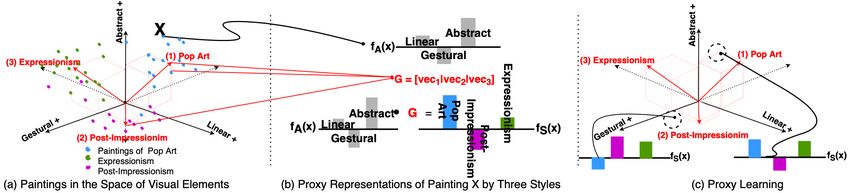
2.2.1    Incorporating Classes as Learning Attributes
Informative dependencies between semantic attributes and objects (class) are useful; in fact, they have co-appeared
in many papers. Lampert et al. [16] assign attributes to images on a per-class basis and train attribute classifiers in
a supervised way. On the other hand, Yu et al. [26] model attributes based on their generalized properties—such as
their proportions and relative strength—with a set of categories and make learning algorithms satisfy them as necessary
conditions. The methods do not require any instance-level attributes for training like this paper method, but learning
visual elements satisfying the constraints of relative proportions among classes is not related to our goal or methodology.
Some researchers [27, 28] propose joint learning frameworks to more actively incorporate class information into attribute
learning. In particular, Akata et al. [29] and Romera-Paredes et al. [14] hierarchically treat attributes as intermediate
features, which serve to describe classes. The systems are designed to learn attributes by bi-directional influences from
class to attributes (top-down) and from image features to attributes (bottom-up) like deep-proxy. However, their single
and linear layering, from image features to their intermediate attributes, are different from the multiple and non-liner
layering in deep-proxy.

2.2.2    Learning Visual Concepts from Styles
Elgammal et al. [7, 8] show that a deep-CNN can learn semantic factors of styles from its last hidden layers by using
a hierarchical structure of deep-CNN. They interpret deep-CNN’s last hidden layer with pre-defined visual concepts
through multiple and separated post-procedures, but deep-proxy simultaneously learns visual elements while machines
are trained for style classification. In the experiment, the method proposed by Kim et al. [8] is compared with deep-proxy
as the name of PCA.

3     Methodology
3.1     Linear Relation

3.1.1    Two Conceptual Spaces
Styles are seldom completely uniform and cohesive, and often carry forward within them former styles and other
influences that are still operating within the work. As explained in The Concept of Style [30], a style can be both a
possibility and an interpretation. It is not a definite quality that inherently belongs to objects, although each of the training
samples are artificially labeled with a unique style. Due to the complex variations of the visual properties of art pieces in
sequential arrangements of times, styles can be overlapped, blended, and merged. Based on the idea, this research begins
with representing paintings with the two entities: a set of m visual elements and a set of n styles. Two conceptual vector
spaces S and A for style and visual elements are introduced, whose each dimension is aligned with their semantic. Two
vector functions, fA (·) and fS (·), are defined to transform input image x into the conceptual spaces in equation (1) below.

                                   fA (x) : x → ~a(x) = [a1 (x), a2 (x), ..., am (x)]t ∈ A
                                                                                                                             (1)
                                    fS (x) : x → ~s(x) = [s1 (x), s2 (x), ..., sn (x)]t ∈ S
Figure 1 and 2 show example paintings that are encoded by visual elements and styles. They are generated by deep-proxy
(using a general relationship estimated by sample means of a few ground truth value).

3.1.2    Category-Attribute Matrix
Inspired by a prototype theory [31] in cognitive science, we posit that a set of pre-defined visual elements of art is
sufficient for characterizing styles. According to this theory, once a set of attributes are arranged to construct a vector
space, a vector point can summarize each of categories. Mathematically modeling the principles, xs∗i is set to be the
typical (best) example for the style si , where i ∈ {1, 2, ...n} and n is the number of styles. This is represented by
fA (x∗si ) = x → ~a(x∗si ). By accumulating the ~a(x∗si ) ∈ Rm as columns for all different n styles, a matrix G ∈ Rm×n is
formed. Matrix G becomes a category-attribute matrix.

3.1.3    Linear System
Matrix G ideally defines n typical points for n styles in the attribute space of A. However, as aforementioned, images that
belong to a specific style show intra-class variations. In this sense, for a painting x that belongs to style si , the fA (x∗si )
is likely to be the closest to the fA (x), and its similarities to other styles’ typical points can be calculated by the inner
products between fA (x) and fA (x∗si ) for all n styles, i ∈ {1, 2, ...n}. All computations are expressed by fA (x)t · G and

                                                               4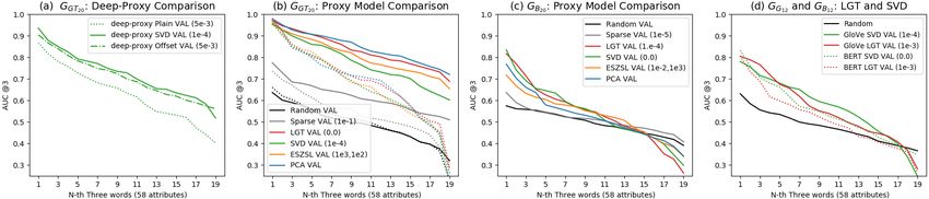
Figure 1: Fire Island by Willem de Kooning (1946): Along with the original style of Abstract Expressionism, Expression-
ism, Cubism, and Fauvism have all left visual traces within the painting. These are earlier styles that De Kooning, the
artist, knew and learned from before developing his own mature style. And the visual traces of the styles are as follows:
the breaking apart of whole forms or objects (Cubism), a loose, painterly touch (Expressionism) and vivid, striking color
choices and juxtapositions such as pink, teal and yellow (Fauvism).

its output fS (x)t . This results in the linear equation (2) below.

                                                    fA (x)t · G = fS (x)t                                            (2)

3.2   Definition of Proxy Learning

In equation (2), knowing fS (·) becomes linearly tied with knowing fA (·), so we have the following questions: (1) given
G and fS (·), how can we learn the function fA (·)? (2) before doing that, how can we properly encode G and fS (·) first?
This paper aims to answer these questions. We first re-define them by a new concept of learning, named proxy learning.
Figure. 3 is an illustrative example to describe it.

   Proxy learning: a computational framework that learns the function fA (·) from fS (·) through a linear relationship G.
G is estimated by language models or human survey.

                                                               5
Figure 2: East Cowes Castle, the seat of J.Nash, Esq. the Regatta beating to windward by J.M.W Turner (1828): The
painting is originally belonged to Romanticism but Realism and Impressionism are also used for its style encoding.

Figure 3: Summary of Proxy Learning: (a) The paintings of three styles (Pop art, Post-impressionism, and Expressionism)
are scattered in the space of three visual elements (abstract, gestural, and linear). The red vectors represent typical vectors
of the three styles. (b) A painting X, originally positioned in the visual space, can be transformed to the three-style
(proxy) representation by computing inner products with each of the typical vectors. (c) Proxy learning aims to estimate
or learn its original visual coordinates from a proxy representation and a set of typical vectors.

3.3   Language Modeling

The G matrix is estimated by using distributed word embeddings in NLP. Two embeddings were considered: GloVe [1]
and BERT [2, 3]. However, their original dictionaries do not provide all the necessary art terms. Especially for BERT,

                                                              6
it holds a relatively smaller dictionary than GloVe. In the original BERT, vocabulary words are represented by several
word-pieces [32], so it is unnecessary to hold a large set of words. However, the token-level vocabulary words could
lose their original meanings, so a new BERT model had to be trained from scratch on a suitable art corpus in order to
compensate for the deficient dictionaries.

3.3.1         A Large Corpus of Art
To prepare a large corpus of art, we first gathered all the descendent categories (about 6500) linked with the parent
categories of “Painting” and “Art Movement” in Wikipedia and scrawled all the texts under the categories by using a
library available in public. Some art terms and their definitions presented in TATE museum 2 were also added, so finally,
with ∼ 2, 400, 000 sentences, a set word embedding set—BERT—is newly trained for art.

3.3.2         Training BERT
For a new BERT model for art, the BERT-BASE model (12-layer, 768-hidden, 12-heads, and not using cased letters) was
selected and trained from scratch with the collected art corpus. For training, the original vocabulary set is updated by
adding some words which are missed in the original framework. We averaged all 12 (layers) embeddings to compute
each of final word embeddings. All details about BERT training is presented in SI B.

3.3.3         Estimation of Category-Attribute Matrix G
To estimate a matrix G, vector representations were collected and the following over-determined system of equations was
set. Let the WA ∈ Rd×m denote a matrix of which each column implies a d-dimensional word embedding to encode one
of m visual elements, and the wsi ∈ Rd be a word embedding that represents style si among n styles.
                                                    WA · ~a(x∗si ) = wsi                                               (3)
By solving the equation (3) for i ∈ {1, 2, ..., n}, the vector ~a(x∗si ) ∈ Rm was estimated, which becomes each column
vector of G. It quantifies how the visual elements are positively or negatively related to a certain style in a distributed
vector space. In general, word embedding geometrically captures semantic or syntactical relations between words, so this
paper postulates that the general relationship among the concepts can be reflected by the linear formulation (3).

3.4        Deep-Proxy

                                             Figure 4: Deep-Proxy Architecture

   We propose a novel method to jointly learn the two multi-modal functions, fS (x) and fA (x), through a pre-estimated
general matrix (G). Its principal mechanism is a category-attribute matrix (G) is hard-coded into the last fully connected
(FC) parameters of a deep-CNN, so it is enforced to learn visual elements (fA (x)) from its last hidden layers, while it is
outwardly trained to learn multiple styles (fS (x)). We propose to name this framework deep-proxy. In this paper, the
original VGG-16 [33] is adapted for its popularity and modified as a style classifier, as shown in Figure 4.

3.4.1         Implementation of Deep-Proxy
All convolution layers are transferred from the ImageNet as is and frozen, but the original FC layers, (4096−4096−1000),
are expanded to the five layers (2048 − 2048 − 1024 − 58 − G∗ (58 × n) − n number of styles). These FC parameters
      2
          http://tate.org.uk/art/art-terms

                                                             7
(cyan colored and dashed box) are updated during training. We also tried to fine-tune convolution parts, but they showed
slightly degraded performance compared to the FC-only training. Therefore, all the results presented in the later sections
are FC-only trained for 200, 000 steps at 32 batch size by the momentum optimizer (momentum = 0.9). The learning
rate is initially set as 1.0e − 3 and degraded at the factor of 0.94 every 2 epochs. The final soft-max output is designed to
encode the fS (x), and the last hidden layer (58-D) is set to encode the fA (x). The two layers are interconnected by the
FC block G∗ (magenta colored and dashed box) to impose a linear constraint between the two modalities. For the fA (x),
the hidden layer’s Rectified Linear Units (ReLU) is removed, so it can have both positive and negative values.

3.4.2   Objective Function of Deep-Proxy
Let I(q, k) be an indicator function stating whether or not the k-th sample belongs to style class q. Let sq (x|w) be the
q-th style component of the soft-max simulating fS (x). Let fA (x|w) be the last hidden activation vector, where x is an
input image and ω is the network’s parameters. Then, an objective for multiple style classification is set as in equation (4)
below. The λ is added to regularize the magnitudes of the last hidden layer.

                                         Q
                                       K X
                                       X
                                 min           −I(q, k) · loge (sq (x|ω)) + λ · kfA (x|ω)k1                              (4)
                                  ω
                                       k   q

In the next subsections, three versions of deep-proxy are defined depending on how G∗ matrix is formulated.

3.4.3   Plain Method (G∗ = G)
A G matrix is estimated and plugged into the network as it is. Two practical solutions are considered to estimate G,
language models and sample means of a few ground truth values. In training for Plain, the G∗ is fixed as the G matrix,
while the other FC layers are updated. This modeling is exactly aligned with equation (2).

3.4.4   SVD Method
A structural disadvantage of Plain method is noted and resolved by using Singular Vector Decomposition (SVD).
   It is natural that the columns of a G matrix are correlated because a considerable number of visual properties are
shared among typical styles. Thus, if the machine learns visual space properly, the multiplication of fA (x)t with G
necessarily produces fS (x)t , which is highly valued on multiple styles. On the other hand, the deep-proxy is trained
by one-hot vectors promoting orthogonality among styles and a sharp high value on a specific style component. Hence,
learning with one-hot vectors can cause interference on learning visual semantics if we simply adopt the plain method
above. For example, suppose there is a typical Expressionism painting x∗ . then, it is likely to be highly valued both on
the Expressionism and Abstract-Expressionism under the equation (2) because the two styles are correlated visually.
But if one hot-vector encourages the machine to value fS (x∗ ) highly on the Expressionism axis only, then the machine
might not be able to learn visual concepts well, such as gestural brush-strokes or mark-making, and the impression of
spontaneity, because those concepts are supposed to be high on Expressionism, too. To fix this discordant structure, the G
and fA (x) are transformed to the space where typical style representations are orthogonal to one another. It reformulates
equation (2) by the equation (5), where T is a transform matrix to the space.
                                               [fA (x)t · T t ] · [T · G] = fS (x)t                                      (5)

    To compute the transform matrix T , G is decomposed by SVD. As the number of attributes (m) is greater than
the number of classes (n), and its rank is n, the G is decomposed by U · Σ · V t , where the U (m × n) and V (n × n)
are the matrices whose columns are orthogonal and the Σ (n × n) is a diagonal matrix. From the decomposition,
V t = Σ−1 · U t · G, so we can use Σ−1 · U t as the transform matrix T . The T = Σ−1 · U t transforms each column of G
to each orthogonal column of V t . In this deep-proxy SVD method, the G∗ is reformulated by these SVD components as
presented in equation (6) below.
                                           G∗ = T t · T · G = U · Σ−2 · U t · G                                     (6)

3.4.5   Offset Method
A positive offset vector ~o ∈ R+m is introduced to learn a threshold to determine a visual concept as relevant or not. Each
component of ~o implies an individual threshold for each of the visual elements, so when it is subtracted from a column
of a G matrix, we can take zero as an absolute threshold to interpret whether or not visual concepts are relevant to a
style class. Since matrix G is often encoded by the values between zero and one, especially when it is created by human
survey (ground truth values), we need a proper offset to shift the G matrix. Hence, the vector ~o ∈ R+m is set as learnable

                                                                8
parameters in the third version of deep-proxy. It sets the G∗ as U · Σ−2 · U t · (G − µ), where µ = [~o|~o|...|~o] is the tiling
matrix of the vector ~o. In Offset method, the SVD components U and Σ are newly calculated for the new (G − µ) at
every batch in training.

4     Experiments
Four pre-existing methods, sparse coding [12], logistic regression (LGT) [13], Principal Component Analysis (PCA)
method [8], and an Embarrassingly Simple approach to Zero-Shot Learning (ESZSL) [14] are reformulated in the context
of proxy learning and quantitatively compared with each other. In this section, we demonstrate how LGT and deep-proxy
based on deep-learning are more robust than others when a general relationship (G matrix) is estimated by language
models; GloVe [1] or BERT [2, 3]. We also show LGT is degraded sensitively, when G matrix is sparse. All detailed
implementations of the four pre-existing methods are explained in SI C.

4.1     Four Proxy Methods

4.1.1    Logistic Regression (LGT) [13]
Each column of G was used to assign attributes to images on a per class basis. When G matrix is not a probabilistic
representation, without shifting zero points, the positives were put into the range of 0.5 to 1.0 and the negatives were put
into the range of 0.0 to 0.5.

4.1.2    PCA [8]
The last hidden feature of a deep-CNN style classifier is encoded by styles and then multiplied with the transpose of G
matrix to finally compute each degree of the visual elements.

4.1.3    ESZSL [14]
This can be regarded as a special case of the deep-proxy Plain by setting a single FC layer between visual features and
fA (x), replacing the softmax loss with Frobenius norm k·k2F ro , and encoding styles with {−1, +1}. To compute the
single layer, a global optimum is found through a closed-form formula proposed by Romera-Paredes et al. [14].

4.1.4    Sparse Coding [12]
It estimates fA (·) directly from the style encodings fS (·) and G matrix by solving a sparse coding equation without
seeing input images. Its better performance versus random cases proves our hypothetical modeling assuming informative
ties between style and visual elements.

4.2     WikiArt Data Set and Visual Elements

This paper used the 76921 paintings in WikiArt’s data set [34] and merged their original 27 styles into 20 styles 3 , the
same as those presented by Elgammal et al. [7]. 120 paintings were separated for evaluation, and the remaining samples
were randomly split into 85% for training and 15% for validation. This paper adopts the pre-selected visual concepts
proposed by Kim et al. [8]. In the paper, 59 visual words are suggested, but we used 58 words, excluding the “medium”
because it is not descriptive.

4.3     Evaluation Methods

4.3.1    Human Survey
A binary ground truth set was completed by seven art historians. The subjects were asked to choose between one of the
following three choices: (1) yes, the shown attribute and painting are related. (2) they are somewhat relevant. (3) no, they
are not related. Six paintings were randomly selected from each of 20 styles, and art historians made three sets of ground
truths of 58 visual elements for the 120 paintings first. From the three sets, a set was determined based on the majority
vote. For example, if a question is marked by three different answers, the (2) ‘somewhat relevant’ is determined as the
final answer. The results show 1652 (24%) as relevant, 782 (11%) as somewhat, and 4526 (65%) as irrelevant. In order to
   3
     Abstract-Expressionism, Art-Nouveau-Modern, Baroque, Color-Field-Painting, Cubism, Early-Renaissance, Expressionism,
Fauvism, High-Renaissance, Impressionism, Mannerism, Minimalism, Naïve-Art-Primitivism, Northern-Renaissance, Pop-Art,
Post-Impressionism, Realism, Rococo, Romanticism, and Ukiyo-e

                                                               9
Figure 5: (a) Three deep-proxy models by GGT20 are compared on “eval”. SVD is selected as the best model for art. (b)
Proxy models by GGT20 are compared. The solid-lines are evaluated by “eval-G”, and the dotted-lines are evaluated by
“eval-N G”. (c) Five proxy models by GB20 are evaluated by “eval”. (d) SVD and LGT by GB12 and GG12 are compared
by “eval-VAL”.

balance positive and negative values, this paper considered the somewhat answers as relevant and created a binary ground
truth set. The 120 paintings will be called “eval” throughout this paper.

4.3.2    AUC Metric
The Area Under the receiver operating characteristic Curve (AUC) was used for evaluation. When we say AUC@K, it
means an averaged AUC score, where the K denotes the number of attributes to be averaged. A random case is simulated
and drawn in every plot as a comparable baseline. Images are sorted randomly without the consideration of the machine’s
out values and then AUCs are computed. We explained why AUC is selected for art instead of other metrics (mAP or PR)
in SI D.

4.3.3    Plots
To draw a plot, we measured 58 AUC scores for all 58 visual elements. The scores were sorted in descending order,
every three scores were grouped, and 19 (b58/3c) points of AUC@3 were computed. Since many of the visual concepts
were not learnable (AUC ≤ 0.5), a single averaged AUC@58 value did not differentiate performance clearly. Hence, the
descending scores were used, but averaged at every three points for simplicity. Regularization parameters were written in
the legend boxes of plots if necessary.

4.3.4    SUN and CUB
SUN [19] and CUB [35] are used to understand the models in general situations. All experiments are based on the
standard splits, proposed by Xian et al. [22]. For evaluation, mean Average Precision (AP) is used because the ground
truth of the data sets is imbalanced by very large negative samples (the mean of all the samples is 0.065 for SUN and 0.1
for CUB at the binary threshold of 0.5). For G matrix, their ground truth samples are averaged.

4.4     Estimation of Category-Attribute Matrix

Two ways to estimate G matrix are considered. First, from the two sets of word embeddings—GloVe and BERT—two G
matrices are computed by equation (3). This paper will refer to the BERT matrix as GB and to the GloVe matrix as GG .
The GG is used only for 12-style experiments in a section later because the vocabulary of GloVe does not contain the all
terms for the 20-style. As necessary, they will be written with the number of styles involved in experiments like GB20
or GB12 . Second, 58-D ground truths of the three paintings, randomly selected among the six paintings of each style,
were averaged and accumulated into columns, and the ground truth matrix GGT was also established. To do so, we first
mapped the three answers of the survey with integers: “relevant” = +1; “somewhat” = 0; and “irrelevant” = −1. The 60
paintings of “eval” used to compute GGT will be called “eval-G” and the others will be called “eval-N G”.

4.5     Quantitative Evaluations

4.5.1    Model Selection for Deep-Proxy
To select the best deep-proxy for art, the three versions of Plain, SVD, and Offset by GGT20 are compared. For Offset, the
GGT20 is pre-shifted by +1.0 to make all components of GGT20 matrix positive, and let machines learn a new offset from
it. For the regularization λ in equation (4), 1e−4, 5e−4, 1e−3, and 5e−3 are tested. In Figure 5 (a), SVD achieved the

                                                           10
best rates and outperformed the Plain model. Offset was not as effective as SVD. Since GGT20 was computed from the
ground truth values, its zero point was originally aligned with “somewhat”, so offset learning may not be needed.
For a comparable result with SUN data, Offset is shown as the best in Figure 6 (a). SUN’s G matrix is computed by
“binary” ground truths, so it is impossible to gauge the right offset. Hence, Offset learning becomes advantageous for SUN.
However, for CUB, SVD and Offset were not learnable (converged to a local minimum, whose recognition is the random
choice of equal probabilities). Since CUB’s G matrix has smaller eigenvalues than other data sets, implying subtle visual
difference among bird classes, the two deep-proxy methods happen to be infeasible by demanding a neural net to capture
fine and local visual differences of birds first, in order to discern the birds as orthogonal vectors. However, for the neural
net especially in the initial stage of learning, finding the right direction to the high goal is far more challenging compared
to the case of art and SUN, whose attributes can be found rather distinctively and globally in different class images. The
detailed results for CUB and SUN are shown in SI E.
4.5.2 Sensitive Methods to Language Models
Proxy models by GGT20 and GB20 are evaluated in Figure 5 (b) and (c). To avoid the bias by the samples used in
computing G matrix, for the models by GGT20 , validation (solid-line) and test (dotted-line) are separately computed
based on “eval-G” and “eval-N G ” each.
High sensitivity to GB20 is observed for PCA and ESZSL. In Figure 5 (b), PCA and LGT show similar performance
on “eval-N G”, but on “eval-G”, PCA performs better than LGT. The same phenomenon is observed between ESZSL and
SVD again. The better performance on “eval-G” indicates somewhat direct replication of G matrix into outcomes. This
hints that ESZSL and PCA can suffer more degradation than other models if G matrix is estimated by language models,
so its imperfection straightly act on their results, as shown in Figure 5 (b) and (c). Since they compute visual elements
through direct multiplications between processed features and G matrix, and particularly for ESZSL, it finds a global
optimum given a G matrix, they showed the highest sensitivity to the condition of G matrix.
4.5.3 Robust Methods to Language Models
Deep-learning makes LGT and deep-proxy slowly adapt to the information given by G matrix, so the models are less
affected by language models than ESZSL and PCA, as shown in Figure 5 (c). LGT can learn some visual elements
through BERT or GloVe, even when not all style relations for the elements are correct in the models. For example, for
GB , ‘expressionism’ is encoded as more related with “abstract” than ’cubism’ or ‘abstract-expressionism’, which is false.
But despite the partial incorrectness, LGT gradually learns the semantic of “abstract” at the rate of 0.84 AUC using the
training data in a larger range of styles, correctly encoded; northern-renaissance (least related to “abstract”) < rococo <
cubism < abstract-expressionism (most related to “abstract”) etc (abstract AUCs of SVD, PCA, and ESZSL by GB20 :
0.9, 0.8, 0.7).
Deep-proxy more actively adjusts some portion of G matrix. Suppose there is a neural net trained with G0 = (G+∆G)
distorted by ∆G. By equation (2), this fA0 (x)t · (G + ∆G) = fSt (x) is a valid convergent point of the net, and we also
can see this (fA0 (x)t + bt (x)) · G = fS (x)t as another possible point, where b(x)t · G = fA0 (x)t · ∆G. If the bottom of
the neural net approximately learns fA0 (x)t + bt (x), it would work as if a better G is given, absorbing some errors. This
adjustment could explain the robustness to the imperfection of language models than others, and also the flexibility to the
sparse G matrix that is shown to be directly harmful for LGT. This will be discussed in the next section.
4.5.4 Logistic and Deep-Proxy on GGT
Two factors are analyzed with LGT and SVD performance: intra-class’s standard deviation (σstd ) and mean (µ). The
intra-statistics of each style are computed with “eval” and averaged across the styles to estimate σstd and µ for 58
visual elements. For LGT and SVD by GGT20 , AUC is moderately related with σstd (Pearson correlation coefficient
rLGT = −0.65 and rSV D = −0.51), but their performance is not explained solely by σstd . As shown in Figure 7 (a),
“monochromatic” (AUC of LGT and SVD: 0.49 and 0.58) scored far less than “flat” (AUC of LGT and SVD : 0.94 and
0.92) even if both words’ σstd are similar and small. Since the element of monochromatic was not a relevant feature
for most of styles, it was consistently encoded as very small values across the styles in GGT matrix. The element has
small variance within a style, but does not have enough power to discriminate styles so failed to learn. LGT can be more
degraded with the sparsity because the information encoded that is close to zero for all styles cannot be back-propagated
properly. As shown in Figure 6 (b), intra-class µ of 102 attributes in SUN are densely distributed between 0.0 and 0.1,
so LGT is lower ranked compared to art. LGT AP is most tied in the sparse µ to others (rLGT = 0.43, rOf f set = 0.36,
rP CA = 0.33, rESZSL = −0.15 at µ < 0.3).
For SVD by GGT20 , its overall performance is lower than LGT by GGT20 . When the words “diagonal”, “parallel”,
“straight”, and “gestural” (four green dots in Figure 7 (a)) were found by the condition of |AU C(SV D) −AU C(LGT ) | > 0.2,
11Figure 6: SUN experiment: (a) Validation results for all models are shown. (b) The relationship between validation-AP
(y-axis) and intra-class µ (x-axis) for LGT is presented for each attribute (each red dot). Points of Offset (two green dots)
are drawn only when the AP-gap between Offset and LGT is more than 0.2. The higher scores on the green dots show
that Offset is less affected by the sparsity of G matrix than LGT. As the AP-gap gets lower to 0.15, 19 words were found,
and Offset worked better than LGT for all the 19 words.
Figure 7: (a) The relationship between test-AUC (y-axis) and σstd (x-axis) and µ (size of dots) for LGT (by GGT20 and
“eval-NG”) is shown for each attribute (each red dot). Offset points (four green dots) are drawn only when the AUC-gap
between the SVD and LGT is more than 0.2. Each performance gap is traced by the blue dotted-lines. (b) Visual elements
scored more than 0.65 AUC by SVD or LGT (by GB20 and “eval”) are presented. (c) Style Encoding of BERT and GloVe
for the word “planar”.
LGT scored higher than SVD for all words. Since SVD is trained by an objective function for multiple style classification,
the learning visual elements can be restricted by the following cases. Some hidden axes could be used to learn non-
semantic features to promote learning styles. Or, some necessary semantics for styles could be strewn throughout multiple
axes. Hence, LGT generally learns more words than SVD when G matrix is estimated by some ground truths as shown in
Figure 5 (b), but G matrix should not be too sparse for LGT.
4.5.5 Logistic and Deep-Proxy on BERT and GloVe
For language models, it is a bit hard to generalize the performance of LGT and SVD. As shown in Figure 7 (b), it was not
clear which is better with BERT. We needed another comparable language model to understand their performance. GloVe
is tested after dividing 20 styles into train (12 styles) 4 and test (8 styles). Aligned with the split, the “eval” was also
separated into “eval-VAL” and “eval-TEST ” (8 unseen styles in training). Here, the “eval-VAL” was used to select hyper
parameters. On the same split, the models by BERT GB12 were compared, too. Depending on each language model, the
ranking relations were differently shown. In Figure 5 (d), SVD by GB12 scored better than LGT at all AUC@3 points.
However, LGT by GG12 was better than SVD for the first top 15 words, but for second 15 words, SVD scored better than
LGT. To figure out a key factor of the different performance, we scored the quality of BERT and GloVe with {−1, +1}
for each visual element and conducted correlation analysis between the scores and the AUC results. Pearson correlation
coefficient r between AUCs and the scores are computed. The results are shown in Figure 8.
4
Baroque, Cubism, Expressionism, Fauvism, High-Renaissance, Impressionism, Mannerism, Minimalism, Pop-Art, and Ukiyo-e
12Figure 8: Correlation analysis between AUCs and matrix scores. The BERT plots of (a-1) and (a-2) are drawn based on
the 22 visual elements which scored more than AUC 0.6 by any of SVD or LGT (by GB12 ). The GloVe plots of (b-1) and
(b-2) are drawn based on the 28 visual elements which scored more than AUC 0.6 by any of SVD or LGT (by GG12 ).
This shows LGT is more sensitively affected by the quality of language models.
In the analysis, GloVe scored higher than BERT, and LGT showed the stronger correlation than SVD between AUCs
and scores. This proves the robustness of SVD to the imperfection of language models along with the results of Fig 5 (d).
As a specific example, the word “planar” is incorrectly encoded by BERT, quantifying some negatives on Expressionism,
Impressionism, and Post-Impressionism as shown by Figure 7 (c). The wrong information influenced more on LGT, so
its AUC scored 0.38 (eval-TEST: 0.47) by BERT but 0.77 (eval-TEST: 0.76) by GloVe, while SVD learned “planar” by
the similar rates of 0.73 (eval-TEST: 0.58) by BERT and 0.78 (eval-TEST: 0.68) by GloVe on “eval-VAL”. For LGT,
the defective information is directly provided through training data, so it is more sensitively affected by noisy language
models. On the other hand, SVD can learn some elements even when it is trained by a G matrix that is not perfect if the
elements are essential for style classification possibly through the adjustment operation, as aforementioned. Another split
of 12-training style 5 vs. 8-test style is also tested by BERT. In this experiment, LGT also scored less than SVD as shown
in Figure 9.
4.5.6 Descending Ranking Results of SVD by GB20
To present some example results, 120 paintings of “eval” are sorted based on the activation values fA (x) of SVD by
GB20 . Table 3 presents some results of words that achieved more than 0.65 or less than 0.65 with BERT model. This
5
Art-Nouveau-Modern, Color-Field-Painting, Early-Renaissance, Fauvism, High-Renaissance, Impressionism, Mannerism,
Northern-Renaissance, Pop-Art, Rococo, Romanticism, and Ukiyo-e
13Figure 9: AUC plots of random split on BERT: SVD by GB12 scored better than LGT at most of AUC@3 points.
shows how the “eval” paintings are visually different according to each output-value of deep-proxy-GB for the selected
seven visual elements (abstract, chromatic, atmospheric, planar, representational, geometric, and perspective).
5 Conclusion and Future Work
Quantifying fine art paintings based on visual elements is a fundamental part of developing AI systems for art, but their
direct annotations are very scarce. In this paper, we presented several proxy methods to learn the valuable information
through its general and linear relations to style, which can be estimated by language models or human survey. They are
quantitatively analyzed to reveal how the inherent structures of the methods make them robust or weak on the practical
estimation scenarios. The robustness of deep-proxy to the imperfection of language models is a key finding. For future
study, we will look at more complex systems. For example, a non-linear relation block learned by language models
could be transferred or transplanted to a neural network to learn visual elements through the deeper relation with styles.
Furthermore, direct applications for finding acoustic semantics for music genres or learning principle elements for fashion
designs would be interesting subjects for proxy learning. Their attributes are visually or acoustically shared to define
higher level of categories, but their class boundaries could be softened as proxy representations.
14Visual Elements (AUC ≥ 0.65) Visual Elements (AUC ≤ 0.65)
abstract chromatic atmospheric planar representational geometric perspective
0.90 0.79 0.75 0.71 0.67 0.63 0.46
Table 3: Descending ranking results (top to bottom) based15on the prediction fA (x) of SVD (GB20 and λ = 0.0). The
five most (1 − 5 rows) and five least (6 − 10 rows) relevant paintings are shown as the machine predicted. The last row
indicates the AUC score of each visual element.References
[1] Jeffrey Pennington, Richard Socher, and Christopher Manning. Glove: Global vectors for word representation.
In Proceedings of the 2014 conference on empirical methods in natural language processing (EMNLP), pages
1532–1543, 2014.
[2] Jacob Devlin, Ming-Wei Chang, Kenton Lee, and Kristina Toutanova. Bert: Pre-training of deep bidirectional
transformers for language understanding, 2018.
[3] Ashish Vaswani, Noam Shazeer, Niki Parmar, Jakob Uszkoreit, Llion Jones, Aidan N Gomez, Łukasz Kaiser, and
Illia Polosukhin. Attention is all you need. In Advances in Neural Information Processing Systems (NIPS 2017),
pages 5998–6008, 2017.
[4] Lois Fichner-Rathus. Foundations of art and design: An enhanced media edition. Cengage Learning, 2011.
[5] Otto G Ocvirk, Robert E Stinson, Philip R Wigg, Robert O Bone, and David L Cayton. Art fundamentals: Theory
and practice. McGraw-Hill, 2002.
[6] John Charles Van Dyke. Principles of Art: Pt. 1. Art in History; Pt. 2. Art in Theory. Fords, Howard, & Hulbert,
1887.
[7] Ahmed Elgammal, Bingchen Liu, Diana Kim, Mohamed Elhoseiny, and Marian Mazzone. The shape of art history
in the eyes of the machine. In Thirty-Second AAAI Conference on Artificial Intelligence, pages 2183–2191. AAAI
press., 2018.
[8] Diana Kim, Bingchen Liu, Ahmed Elgammal, and Marian Mazzone. Finding principal semantics of style in art. In
2018 IEEE 12th International Conference on Semantic Computing (ICSC), pages 156–163, 2018.
[9] Hui Mao, Ming Cheung, and James She. Deepart: Learning joint representations of visual arts. In Proceedings of
the 25th ACM international conference on Multimedia (ACMMM), pages 1183–1191. ACM, 2017.
[10] Igor E Berezhnoy, Eric O Postma, and Jaap van den Herik. Computerized visual analysis of paintings. In Int. Conf.
Association for History and Computing, pages 28–32, 2005.
[11] C Richard Johnson, Ella Hendriks, Igor J Berezhnoy, Eugene Brevdo, Shannon M Hughes, Ingrid Daubechies, Jia
Li, Eric Postma, and James Z Wang. Image processing for artist identification. IEEE Signal Processing Magazine,
25(4):37–48, 2008.
[12] Bradley Efron, Trevor Hastie, Iain Johnstone, Robert Tibshirani, et al. Least angle regression. The Annals of
statistics, 32(2):407–499, 2004.
[13] Emine Gul Danaci and Nazli Ikizler-Cinbis. Low-level features for visual attribute recognition: An evaluation.
Pattern Recognition Letters, 84:185–191, 2016.
[14] Bernardino Romera-Paredes and Philip Torr. An embarrassingly simple approach to zero-shot learning. In
Proceedings of the 32nd International Conference on Machine Learning (PMLR), pages 2152–2161, 2015.
[15] Ali Farhadi, Ian Endres, Derek Hoiem, and David Forsyth. Describing objects by their attributes. In Proceedings of
the IEEE Conference on Computer Vision and Pattern Recognition (CVPR), pages 1778–1785. IEEE, 2009.
[16] Christoph H Lampert, Hannes Nickisch, and Stefan Harmeling. Attribute-based classification for zero-shot visual
object categorization. IEEE Transactions on Pattern Analysis and Machine Intelligence (TPAMI), 36(3):453–465,
2013.
[17] Vittorio Ferrari and Andrew Zisserman. Learning visual attributes. Advances in Neural Information Processing
Systems (NIPS 2007), 20:433–440, 2007.
[18] Sukrit Shankar, Vikas K Garg, and Roberto Cipolla. Deep-carving: Discovering visual attributes by carving deep
neural nets. In Proceedings of the IEEE conference on computer vision and pattern recognition (CVPR), pages
3403–3412, 2015.
[19] Genevieve Patterson, Chen Xu, Hang Su, and James Hays. The sun attribute database: Beyond categories for deeper
scene understanding. International Journal of Computer Vision, 108(1-2):59–81, 2014.
[20] Devi Parikh and Kristen Grauman. Relative attributes. In Proceedings of the 2011 International Conference on
Computer Vision (ICCV), pages 503–510. IEEE, 2011.
[21] Shugao Ma, Stan Sclaroff, and Nazli Ikizler-Cinbis. Unsupervised learning of discriminative relative visual attributes.
In European Conference on Computer Vision (ECCV), pages 61–70. Springer, 2012.
[22] Yongqin Xian, Christoph H Lampert, Bernt Schiele, and Zeynep Akata. Zero-shot learning—a comprehensive
evaluation of the good, the bad and the ugly. IEEE transactions on pattern analysis and machine intelligence
(TPAMI), 41(9):2251–2265, 2018.
16[23] Li-Jia Li, Hao Su, Yongwhan Lim, and Li Fei-Fei. Objects as attributes for scene classification. In European
Conference on Computer Vision (ECCV), pages 57–69. Springer, 2010.
[24] Chen Huang, Chen Change Loy, and Xiaoou Tang. Unsupervised learning of discriminative attributes and visual
representations. In Proceedings of the IEEE Conference on Computer Vision and Pattern Recognition (CVPR),
pages 5175–5184, 2016.
[25] Huizhong Chen, Andrew Gallagher, and Bernd Girod. Describing clothing by semantic attributes. In European
Conference on Computer Vision (ECCV), pages 609–623. Springer, 2012.
[26] Felix X Yu, Liangliang Cao, Michele Merler, Noel Codella, Tao Chen, John R Smith, and Shih-Fu Chang. Modeling
attributes from category-attribute proportions. In Proceedings of the 22nd ACM international conference on
Multimedia (ACMMM), pages 977–980. ACM, 2014.
[27] Dhruv Mahajan, Sundararajan Sellamanickam, and Vinod Nair. A joint learning framework for attribute models
and object descriptions. In Proceedings of the 2011 International Conference on Computer Vision (ICCV), pages
1227–1234. IEEE, 2011.
[28] Xiaoyang Wang and Qiang Ji. A unified probabilistic approach modeling relationships between attributes and
objects. In Proceedings of the 2013 International Conference on Computer Vision (ICCV), pages 2120–2127. IEEE,
2013.
[29] Zeynep Akata, Florent Perronnin, Zaid Harchaoui, and Cordelia Schmid. Label-embedding for attribute-based
classification. In Proceedings of the IEEE Conference on Computer Vision and Pattern Recognition (CVPR), pages
819–826, 2013.
[30] Berel Lang. The concept of style. Cornell University Press, 1987.
[31] Gregory Murphy. The big book of concepts. MIT press, 2004.
[32] Yonghui Wu, Mike Schuster, Zhifeng Chen, Quoc V Le, Mohammad Norouzi, Wolfgang Macherey, Maxim Krikun,
Yuan Cao, Qin Gao, Klaus Macherey, and othersa. Google’s neural machine translation system: Bridging the gap
between human and machine translation, 2016.
[33] Karen Simonyan and Andrew Zisserman. Very deep convolutional networks for large-scale image recognition. In
International Conference on Learning Representations (ICLR), 2015.
[34] WikiArt. Wikiart: Visual art encyclopedia. http:// www.wikiart.org, 2010. Accessed:2019-12-01.
[35] C. Wah, S. Branson, P. Welinder, P. Perona, and S. Belongie. The caltech-ucsd birds-200-2011 dataset. Technical
Report CNS-TR-2011-001, California Institute of Technology, 2011.
17Supplementary Information (SI)
A Painting Information
Painting Information Painting Information
title: Madonna Conestabile title: The Architect, Jesus T. Acevedo
author: Raphael author: Diego Rivera
year: 1502 year: 1915
style: High Renaissance style: Cubism
title: The Sistine Madonna title: Water of the Flowery Mill
author: Raphael author: Arshile Gorky
year: 1513 year: 1944
style: High Renaissance style: Abstract Expressionism
title: Judith title: Pendulum
author: Gorreggio author: Helen Frankenthaler
year: 1512-1514 year: 1972
style: High Renaissance style: Abstract
title: Morning in a Village title: Untitled Vessel #10
author: Fyodor Vasilyev author: Denise Green
year: 1869 year: 1977
style: Realism style: Neo-Expressionism
title: Forest Landscape with Stream title: Untitled No. 40
author: Ivan Shishkin author: Claude Viallat
year: 1870-1880 year: 1996
style: Realism style: Color-Field-Painting
Table A.1: Information of title, author, year of made, and style
B BERT Model
B.1 Training BERT
For a new BERT model for art, the BERT-BASE model (12-layer, 768-hidden, 12-heads, and not using cased letters) was
selected and trained from scratch over the collected art corpus. For training, the original BERT vocabulary is updated by
adding new words. Table B.1 shows the words that are newly added. For optimizer, Adam algorithm with decay
18List of Words
non-representational, representational, meandering, gestural
amorphous, biomorphic, planar, chromatic
monochromatic, bumpy, art-nouveau, cubism
expressionism, fauvism, abstract-expressionism
color-field-painting, minimalism, naive-art, ukiyo-e
early-renaissance, pop-art, high-renaissance, mannerism
northern-renaissance, rococo, romanticism, impressionism
post-impressionism
Table B.1: 28 words newly added to the original dictionary of BERT
is used. The BERT model is trained for 5e+5 steps with the learning rate of 1.0e−4 and the number of warm-up
steps is set to 1e+4.
B.2 Collecting BERT Embedding
Context-free embedding is collected for each of art terms (20 styles and 58 visual elements). The context-free means only
a target word is inputted to BERT to collect word-embedding without accompanying other words. Each target word is
enclosed only by [CLS] and [SEP] and inputted to the BERT as the format of “[CLS] target-word [SEP]”. 12 output
vectors (768-D) from all 12 hidden layers are collected and averaged. The representations corresponding to the [CLS]
and [SEP] are discarded so only the vector representations for input words are taken as the final embedding. We also tried
to average the embeddings collected only from the top or bottom four layers, but all 12 embeddings were slightly better at
presenting the general relationship between styles and visual elements.
Figure B.1: A general relation between 58 visual elements and 20 styles is estimated by BERT. It is visualized in
gray-scale.
B.3 Visualization of BERT matrix
The general relation estimated by BERT is visualised in gray-scale in Figure B.1. In this figure, the birther square shows
the stronger association between styles and visual elements.
19C Four Proxy Models
C.1 Sparse Coding
Sparse coding [12] is the simplest model for proxy learning, which estimates the visual information from style encodings
without seeing input paintings. By treating the rows of G matrix as over-complete bases of style space S (the number of
styles in this paper is at most 20 and the number of visual elements is 58), ia (fA (x)) is estimated from given G and
fS (x) by sparse coding equation (7) below.
arg minkfS (x) − Gt · ia k2 + λs · kia k1 (7)
ia
To encode a painting x into mutliple styles (fS (x)), the soft-max output of a style classifier is used. To imple-
ment a style classifier, VGG-16 ImageNet’s [33] all convolution layers are transferred as is and frozen, but its original
FC layers (4096 − 4096 − 1000) are modified to five FC layers (4096 − 4096 − 1024 − 512 − n number of styles)
and their parameters are updated in training. The hyper-parameter λs tried during development are 0.0, 1e−1,
1e−2, 1e−3, 1e−4, 1e−5, 0.15, 0.3, 0.45. The linear equation (7) is solved by Least Angle Regression [12].
C.2 Logistic Regression
Logistic regression [13] (LGT) is used to learn visual elements in a sort of supervised way. Similar to the work of
Lampert et al. [16], each column of G was used to assign attributes to images on a per class basis. Each column index
was determined based on the style label. When G matrix are not probabilistic representations, without shifting zero points,
the positives were put into the range of 0.5 to 1.0 and the negatives were put into the range of 0.0 to 0.5. Finally, the
values were adjusted from zero to one.
The logistic regression is implemented on the last convolution layer of a VGG-16 ImageNet. After adding multiple FC
layers (2048 − 2048 − 1024 − 58) on the top of the convolution layer, same as deep-proxy, and the FC parts are newly
updated by an objective function. Let I(q, k) be an indicator function that states whether or not the k-th sample belongs
to style class q. Let g~q (58-D) be the probabilistic representation of a column of G matrix corresponding to q style class.
Let ~l(x|ω) be a (58-D) logistic output of the network, where x is an input image, ω implies the network’s parameter, and
ω1024×58 denotes the last FC layer. Then, an objective function for logistic regression is set as in equation (8) below.
X Q
K X n o
min −I(q, k) · g~q t · loge (~l(x|ω)) + (~158 − g~q )t · loge (~158 − ~l(x|ω)) + λL · kω1024×58 k1 (8)
ω
k q
The λL (regularization) is added to reduce undesirable correlations among attributes by restricting the magnitudes of
the last layer parameters. Tested λL s are 0.0, 1e−3, 1e−4, and 1e−5. All logistic models are trained for 200,000 steps at
32 batch size by a momentum optimizer. Their learning rates are initially set as 1e−3 and degraded at the factor of 0.94
every two epochs as same as deep-proxy.
C.3 PCA
Kim et al. [8] proposed a framework based on Principal Component Analysis (PCA) to annotate paintings with a set of
visual concepts. Differently to proxy learning, they consider a style conceptual space as a joint space where paintings and
each visual concept can be properly encoded to measure their associations. Even though its approach to style space is
different from proxy learning, PCA method can be reproduced in the context of proxy learning as follows.
1. PCA transform of visual embedding The visual embedding, collected from the last hidden layer (before
activation) of a deep-CNN (style classification model), is transformed to PCA space. A VGG-16 style classi-
fication model (FC part : 4096 − 4096 − 1024 − 512) proposed by Elgammal et al. [7] is used to collect the
embedding. Let us denote d is the dimension of the embedding, k is the number of painting samples, and p is
the number of PCA components that cover 95% variance of the embedding. The last layer’s hidden embedding
E ∈ Rd×k is collected, and then PCA projection matrix P ∈ Rp×d (without whitening) is computed from E.
Then, E − [m|~ m|...|
~ ~ is transformed to PCA samples V ∈ Rp×k by equation (9) below, where m
m] ~ ∈ Rd is a
sample mean of E, and m = [m| ~ m|...|
~ m]
~ is the tiling matrix of m.
~
V = P · (E − m) (9)
20You can also read