From Contours to 3D Object Detection and Pose Estimation
←
→
Page content transcription
If your browser does not render page correctly, please read the page content below
in Proc. 13th International Conference on Computer Vision (ICCV), Barcelona, Spain, 2011

                   From Contours to 3D Object Detection and Pose Estimation

                                                 Nadia Payet and Sinisa Todorovic
                                                     Oregon State University
                                                   Corvallis, OR 97331, USA
                                  payetn@onid.orst.edu, sinisa@eecs.oregonstate.edu

                            Abstract                                         to readily dismiss viewpoint-dependent approaches seems
                                                                             too hasty.
    This paper addresses view-invariant object detection and                    In this paper, we revisit the viewer-centered framework.
pose estimation from a single image. While recent work fo-                   We are motivated by two widely recognized findings in
cuses on object-centered representations of point-based ob-                  psychophysics and cognitive psychology that: (i) shape is
ject features, we revisit the viewer-centered framework, and                 one of the most categorical object properties [3], and (ii)
use image contours as basic features. Given training ex-                     viewpoint-dependent object representations generalize well
amples of arbitrary views of an object, we learn a sparse                    across members of perceptually-defined classes [20]. These
object model in terms of a few view-dependent shape tem-                     findings motivate our new approach that uses a number of
plates. The shape templates are jointly used for detecting                   viewpoint-specific shape representations to model an object
object occurrences and estimating their 3D poses in a new                    category. Shape is typically more invariant to color, tex-
image. Instrumental to this is our new mid-level feature,                    ture, and brightness changes in the image than other fea-
called bag of boundaries (BOB), aimed at lifting from indi-                  tures (e.g., interest points), and thus generally enables a
vidual edges toward their more informative summaries for                     significant reduction in the number of training examples,
identifying object boundaries amidst the background clutter.                 required to maintain high recognition accuracy. In this pa-
In inference, BOBs are placed on deformable grids both in                    per, we show that using contours as basic object features
the image and the shape templates, and then matched. This                    allows a sparse multi-view object representation in terms of
is formulated as a convex optimization problem that accom-                   a few shape templates, illustrated in Fig. 1. The templates
modates invariance to non-rigid, locally affine shape defor-                 are specified as 2D probabilistic maps of viewpoint-specific
mations. Evaluation on benchmark datasets demonstrates                       object shapes. They can be interpreted as “mental images”
our competitive results relative to the state of the art.                    of an object category that are widely believed to play an im-
                                                                             portant role in human vision [14]. While the templates are
                                                                             distinct, they are jointly analyzed in our inference. Given
1. Introduction                                                              only a few of these shape templates, we show that it is possi-
   We study multi-view object detection and pose esti-                       ble to accurately identify boundaries and 3D pose of object
mation in a single image. These problems are challeng-                       occurrences amidst background clutter.
ing, because appearances of 3D objects may differ signifi-                       Instrumental to the proposed shape-based 3D object
cantly within a category and when seen from different view-                  recognition is our new, mid-level feature, called bag of
points. A majority of recent work resorts to the object-                     boundaries (BOB). A BOB located at a given point in the
centered framework, where statistical generative models                      image is a histogram of boundaries, i.e., the right image
[16, 22, 17, 1, 10, 7], discriminative models [6], or view-                  contours that occur in the BOB’s neighborhood and belong
independent implicit shape models [15, 18] are used to en-                   to the foreground. If the object occurs, its boundaries will
code how local object features (e.g. points or edgeless), and                be “covered” by many BOBs in the image. Therefore, we
their spatial relationships vary in the images as the cam-                   represent the image and the shape templates of the object
era viewpoint changes. They strongly argue against certain                   model by deformable 2D lattices of BOBs which can collec-
limitations of viewer-centered approaches that apply sev-                    tively provide a stronger support of the occurrence hypothe-
eral single-view detectors independently, and then combine                   sis than any individual contour. This allows conducting 3D
their responses [21, 13]. In the light of the age-long debate                object recognition by matching the image’s and template’s
whether viewer- or object-centered representations are more                  BOBs, instead of directly matching cluttered edges in the
suitable for 3D object recognition [4, 20], the recent trend                 image and the shape templates. There are two main differ-

                                                                         1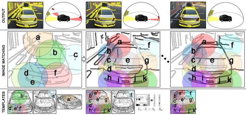
in Proc. 13th International Conference on Computer Vision (ICCV), Barcelona, Spain, 2011

Figure 1. Overview of our approach. We seek a subset of foreground image contours, referred to as boundaries, that jointly best match to the
shape templates of the object model, under an arbitrary affine projection. Instead of directly matching individual contours, we match their
summaries—our new, mid-level features, called bags of boundaries (BOBs). (a) A test image, and the shape templates of the category car.
(b) Successive iterations of matching BOBs placed on deformable grids in the test image (magenta) and the shape templates (yellow). Top:
current estimates of boundaries that best match to the shape templates. Middle: matches from the previous iteration define how to project
the grids of BOBs of every shape template (yellow) onto the test image, and thus match them to the grid of BOBs in the image (magenta);
the grids are deformable to accommodate invariance to non-rigid, locally affine shape deformations of object occurrences. Bottom: current
estimates of the best matching shape template and its affine projection onto the test image. (c) Our results: boundary detection and 3D pose
estimation of the car occurrence in the test image. The estimated viewpoint is depicted as the green camera, and the best matching shape
template is shown as the orange camera. The label “front-left” is our discrete viewpoint estimate.

ences from other common mid-level features (e.g., Bag of                     and the shape templates learned in Step 1. The matching
Words, shape context). First, boundaries, which we use for                   seeks a subset of foreground image contours, i.e., bound-
computing the BOB histogram, are not observable, but hid-                    aries, that jointly best match to the shape templates under
den variables that must be inferred. The BOB histogram is                    an arbitrary affine projection (3D rotation, translation, and
computed from the right contours, not any edges (as in, e.g.,                scale). We lift from the clutter of image edges, and realize
BOW, shape context). Second, BOBs lie on a deformable                        shape matching by establishing correspondences between
2D lattice, whose warping is iteratively guided top-down                     2D lattices of BOBs in the image and the templates. This
by the inference algorithm, such that the BOBs could better                  is formulated as an efficient convex optimization that al-
summarize boundaries for recognition.                                        lows for non-rigid, locally affine, shape deformations. The
                                                                             best matching BOBs identify object boundaries, and the as-
   Overview: Our approach consists of two steps, illus-                      sociated affine projection of the template onto the image.
trated in Fig. 1. In Step 1, we learn the viewer-centered                    The parameters of this affine projection are taken as a real-
shape templates of an object category. We assume that train-                 valued, continuous estimate of 3D object pose, while the
ing images are labeled with bounding boxes around object                     best matching template identifies a discrete pose estimate.
instances. For each training image, we estimate its corre-                      In the following, Sec. 2 points out our contributions;
sponding 3D camera location on the viewing sphere using a                    Sec. 3 describes the viewer-centered shape templates; Sec. 4
standard SfM method. For each camera viewpoint, the tem-                     specifies BOBs; Sec. 5 and Sec. 6 formulate BOB matching;
plate is learned from boundaries detected within the bound-                  and Sec. 7 presents our empirical evaluation.
ing boxes around training instances, seen from that view-
point. After normalizing the bounding boxes to have the                      2. Our Contributions and Prior work
same size as the template, their boundaries are copied to the
template, and averaged. Every pixel in the template counts                      To our knowledge, this paper presents the first shape-
the average frequency it falls on a boundary, resulting in a                 based approach to view-invariant object detection and pose
probabilistic shape map (see Fig. 2). In Step 2, we con-                     estimation from a single image. While most prior work de-
duct shape matching between all contours in a given image,                   tects only bounding boxes around objects [16, 22, 17, 1, 10,

                                                                         2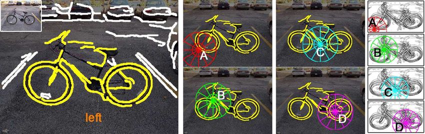
in Proc. 13th International Conference on Computer Vision (ICCV), Barcelona, Spain, 2011

15, 18, 21, 13], our approach is capable of detecting bound-
aries that delineate objects, and their characteristic parts,
seen from arbitrary viewpoints. For delineating object parts,
we do not require part labels in training. The approach of
[7] also seeks to delineate detected objects. However, they
employ computationally expensive inference of a genera-
tive model of Gabor-filter responses only to detect sparsely
placed stick-like edgelets belonging to objects. By using
contours instead of point-based features, we relax the strin-
gent requirement of prior work that objects must have sig-
nificant interior texture to carry out geometric registration.
    We relax the restrictive assumption of some prior work
(e.g., [17]) that objects are piece-wise planar, spatially re-
lated through a homography. We allow non-rigid object de-
                                                                             Figure 2. Example shape templates obtained for the mug category.
formations, and estimate the affine projection matrix.
                                                                             Boundaries that fall in the bounding box of the object are averaged
    Our approach is fundamentally viewer-centered, because                   to form the probabilistic shape map.
we use a set of distinct object representations corresponding
to different camera viewpoints. However, we do not use the
two-stage inference common in prior work [21, 13], where                     cover different sets of contours, and thus change their asso-
one first reasons about objects based on each viewpoint rep-                 ciated histograms, as desired.
resentation independently, and then fuses these hypotheses
in the second stage. Instead, our inference jointly considers                3. Building the Shape Templates
all distinct object representations within a unified convex
optimization framework.                                                         This section explains how to build the shape template
                                                                             from a given set of training images captured from a specific
    Shape-based single-view object detection has a long-
                                                                             camera viewpoint. We will consider that the camera view-
track record in vision (e.g., [2, 5, 23]). The key research
                                                                             point is given together with bounding boxes around objects,
questions explored by this line of work concern the formula-
                                                                             for clarity. In Sec. 7, we relax this assumption, and describe
tion of shape representation and similarity for shape match-
                                                                             how to estimate camera viewpoints of training images.
ing. Similar to the work of [2, 23], we use a lattice of mid-
                                                                                In each training image, we first extract long, salient con-
level shape features, called BOBs, for shape matching. Un-
                                                                             tours, using the approach of [23]. This is illustrated in
like shape context, a BOB is aimed at filtering the clutter of
                                                                             Fig. 2. Then, we set the size of our template to an aver-
image edges, and identifying and summarizing boundaries
                                                                             age rectangle of all training bounding boxes (i.e., the length
that occur in the BOB’s neighborhood. For object detec-
                                                                             of each side of the template is equal to the average length of
tion, we find the best matching subset of BOBs to our shape
                                                                             the corresponding sides of the bounding boxes). All training
templates, such that the matched BOBs maximally cover all
                                                                             bounding boxes are scaled to have the same size as the tem-
image contours that are estimated to be boundaries. This is
                                                                             plate. This allows us to directly copy all boundaries from
very different from most prior work on shape (e.g., [2]) that
                                                                             the bounding boxes to the template. Every pixel in the tem-
typically works with edge fragments, and seeks evidence
                                                                             plate counts the average number of times it falls on a bound-
for their matching in relatively short-range neighborhoods.
                                                                             ary. This results in a probabilistic shape map, as shown in
Instead, we treat each contour as a whole unit, and require
                                                                             Fig. 2. As can be seen, due to the alignment and scaling
a joint support from multiple BOBs to either match it to
                                                                             of bounding boxes, the shape template is capable of captur-
our model, or declare it as the background. This makes our
                                                                             ing prominent object boundaries. Any contours that come
shape matching more robust to background clutter.
                                                                             from background clutter or belong to rare variations of the
    Our shape matching simultaneously estimates a 3D                         object category, by definition, will have low probability of
affine projection of the best matching shape templates to                    occurrence in the shape template.
the image. Related to ours is prior work on matching two                        In this way, we learn a number of shape templates corre-
images under 2D locally affine transformation [9], or global                 sponding to distinct viewpoints present in the training set.
2D scale and rotation transformation [8]. However, they
treat descriptors of image features as fixed vectors, and do                 4. Shape Representation
not account that they change under local or global affine
transformations. By contrast, we allow non-rigid deforma-                       Our shape representation is designed to facilitate match-
tions of contours by estimating the optimal placement of                     ing between image contours, and all shape templates of the
BOBs in the image. As the BOBs change positions, they                        object category. We formulate this matching as many-to-

                                                                         3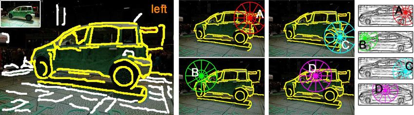
in Proc. 13th International Conference on Computer Vision (ICCV), Barcelona, Spain, 2011

many, because, in general, specific features of a category                   and qj , are represented by 3 × 1 and 4 × 1 vectors, respec-
instance, and canonical features of the category model may                   tively. We want to estimate an n × m matrix F = [fij ],
not be in one-to-one correspondence. Thus, our goal is to                    whose each element fij represents confidence that 2D point
identify a subset of image contours and a subset of template                 i ∈ I is the best match to 3D point j ∈ M.
parts that match. Instead of directly matching contours, we                     The criterion that best matching BOBs have maximally
match BOBs placed on deformable grids in the image and                       similar boundary histograms can be formalized as
all the templates, as illustrated in Fig. 3. The BOBs serve to                          P      P
                                                                                 min       i∈I    j∈M fij cij
jointly collect evidence on candidate boundaries, and facil-                       F                    P              P              (2)
itate many-to-many shape matching.                                               s.t    ∀i, j, fij ≥ 0,     i fij = 1,   j fij ≤ 1,
    A BOB that is placed in the shape template is the stan-
                                                                             where the constraints on the fij ’s enforce one-to-many
dard shape context [2], computed over a relatively large spa-
                                                                             matching, such that every BOB in the template finds its cor-
tial neighborhood. The radius of every BOB in the template
                                                                             responding image BOB. cij is the histogram dissimilarity of
is data-driven and varies in inference, as described in Sec. 5.
                                                                             BOBs i and j defined as
    A BOB that is placed in the image differs from the stan-
dard shape context in that its log-polar histogram includes                                cij;X = (Vi X − Sj )T Σ−1
                                                                                                                  j (Vi X − Sj )       (3)
only those image contours occurring in its neighborhood
that are estimated as boundaries. Similar to the work of                     where the indicator vector of boundaries in the image X ∈
                                                                                    n
[23], we avoid enumerating exponentially many choices of                     {0, 1} , the BOB’s neighborhood matrix Vi , and the bound-
figure/ground labeling of contours. Rather, for a BOB lo-                    ary histogram Sj are defined in Sec. 4. The covariance ma-
cated at image point i, we compute the BOB’s histogram,                      trix Σj is learned in training for each template point j ∈ M.
Si , as the following linear function of an indicator vector,                We organize dissimilarities cij;X in an n × m matrix CX .
X, indexed by all contours in the image, and a matrix Vi ,                   This allows expressing
                                                                                                  P theP  objective of (2) in a more conve-
                                                                                                                                  T
which serves to formalize the BOB’s neighborhood:                            nient matrix form: i∈I j∈M fij cij;X = tr{CX           F }.
                                                                                 To identify boundaries, i.e., estimate X, we extend (2) as
                            Si = Vi X.                             (1)                  T
                                                                                min tr{CX F}
                                                                                F,X
An element of X is set to 1 if the corresponding contour                        s.t    F ≥ 0, F T 1n = 1m , F 1m ≤ 1n , X ∈ [0, 1]n
is estimated as foreground, or 0, otherwise. An element of                                                                             (4)
Vi , denoted as (Vi )st , counts the number of pixels of tth                 where 1n is n-dimensional vector with all 1’s, and X is
contour that fall in sth bin of the log-polar neighborhood                   relaxed to take continuous real values in [0, 1]n .
of i. Note that Vi is observable. However, computing Si                          The formulation in (4) has two major limitations. First,
requires estimation of the hidden variables X in inference.                  the resulting matches may contain template BOBs from all
                                                                             viewpoints, which would mean that the image shows all
5. Shape Matching                                                            object views at once. Therefore, it is necessary to addi-
                                                                             tionally constrain (4), such that a majority of correspon-
    This section presents our inference, under non-rigid                     dences are established between the image and a cluster of
shape deformations and arbitrary 3D affine projection. We                    templates corresponding to neighboring camera locations
place a number of BOBs in the image and the shape tem-                       on the viewing sphere (or, in a special case, one particu-
plates, and match them, as illustrated in Fig. 3. The result                 lar template). The best matching subset of templates can be
is a subset of best matching image BOBs which are closest                    jointly used to robustly estimate the object viewpoint, which
to the expected affine projections of the corresponding tem-                 may have not been seen previously in training. Second, (4)
plate BOBs onto the image. Also, the corresponding pairs                     does not provide invariance to non-rigid shape deformations
of BOBs have the smallest differences in their associated                    and 3D affine transformations. Both limitations could be
boundary histograms. To jointly minimize these two cri-                      addressed by allowing image BOBs to iteratively move to
teria, we estimate the optimal placement of image BOBs                       the expected affine projections of their corresponding tem-
to maximally cover the identified object boundaries, and                     plate BOBs. This is similar to the EM algorithm. For com-
thus account for any non-rigid shape deformations. In the                    puting the expected locations of BOBs (E-step), we maxi-
following, we gradually formalize the matching of BOBs                       mize their matches (M-step). The iterative displacements of
from a simple standard linear assignment problem to the                      image BOBs are constrained to be locally similar. In this
desired complex optimization which allows for non-rigid                      way, we enforce that image BOBs match to the shape tem-
shape transformations.                                                       plates with similar (neighboring) viewpoints on the viewing
    More formally, let M be the set of template BOBs,                        sphere. Below, we specify these additional constraints.
m = |M|, and I be the set of image BOBs, n = |I|. The                            Let T be a set of all projection matrices, so T ∈ T has
homogenous coordinates of image and template BOBs, pi                        the form T = K [R|t], where R is a 3 × 3 rotation matrix,

                                                                         4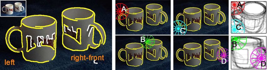
in Proc. 13th International Conference on Computer Vision (ICCV), Barcelona, Spain, 2011

t is a 3 × 1 translation vector, and K captures scale and                    the orthogonality constraint RRT = I to the norm con-
camera parameters. Given T ∈ T that projects the template                    straint kRk∞ ≤ 1. This can be done without affecting the
                           P location of image point pi can
onto the image, the expected                                                 original optimization problem (see [12] for details). kRk∞
be estimated as p̂i;T = j∈M fij T qj . After finding best                    is the spectral norm of R. After T is determined, we
correspondences F = [fij ], we move each pi to its expected                  transformP the image BOBs pi to their expected locations
location p̂i;T , and then repeat matching. The criterion that                p̂i;T = j∈M fij T qj .
neighboring BOBs should have the same displacements can                          (3) We fix T and F , and compute X, and CX .
be formalized as                                                                 (4) Steps (1)–(3) are iterated. After convergence, i.e.,
             X                     X                                         when F, T and X no longer change, we remove the bound-
       min        k(p̂i;T − pi ) −   wik (p̂k;T − pk )k, (5)                 aries indicated by X from the initial set of image contours.
         T ∈T
                i∈I                  k∈I                                         (5) To detect multiple object occurrences in the image,
                                                                             steps (1)–(4) are repeated until the set of image contours
where k·k is ℓ2 norm, and the wik ’s are elements of the n×n
                                                                             reduces to the 10% of its initial size.
adjacency matrix of image BOBs, W = [wik ], representing
                                                                             Implementation. On average, we extract around 80 con-
the neighbor strength between all BOB pairs, (i, k) ∈ I ×
                                                                             tours in each image. Our Matlab CVX implementation of
I. We specify wik as inversely proportional to the distance
                                                                             the above steps (1)–(5) takes about 3min on a 2.66GHz,
between pi and pk .
                                                                             3.49GB RAM PC.
   The objective in (5) minimizes only the magnitude of
relative displacements of BOBs in the image. We also want
to bound their absolute displacements as
                                                                             7. Results
                        X                                                       Datasets. We evaluate our approach on the 3D object
                    min     kp̂i;T − pi k.                (6)                dataset [16] and the Table Top dataset of [18]. The 3D
                      T ∈T
                             i∈I                                             object dataset is used for evaluating on classes cars and
By introducing a 3 × n matrix of image coordinates P , and                   bikes; whereas the Table Top dataset is used for evaluat-
                                                                             ing on classes staplers, mugs and computer mice. In both
a 4 × m matrix of template coordinate Q, we combine the
objectives of (4), (5), and (6) into our final formulation:                  datasets, each class contains 10 object instances. The first 5
                                                                             are selected for training, and the remaining 5 for testing, as
                                                                             in [16, 7, 18]. In the 3D object dataset, each instance is ob-
               T
    min tr CX       F + αkT QF T − P k
   X,F,T                                                                     served under 8 angles (A1 ..A8 ), 2 heights (H1 , H2 ), and 3
                +βk(T QF T − P ) − (T QF T − P )W T k                        scales (S1 ..S3 ), i.e. 48 images. For training, we use only the
                                                                   (7)
                         N
                                                                             images from scale S1 . For testing, we use all 5 × 48 = 240
   s.t          X ∈ [0, 1] ; T ∈ T                                           images per category. In the Table Top dataset, each instance
                F ≥ 0; F T 1N = 1M ; F 1M ≤ 1N                               is observed under 8 angles (A1 ..A8 ), 2 heights (H1 , H2 ),
                                                                             and one scale (S1 ), i.e. 16 images. For cars, we also eval-
    Note that when α = β = 0 and Σj is the identity matrix,
                                                                             uate our method on the PASCAL VOC 2006 dataset, and
(7) is equivalent to the 2D shape packing of [23]. Also, (7)
                                                                             on the car show dataset [13]. The PASCAL dataset con-
is similar to recent matching formulations, presented in [9,
                                                                             tains 544 test images. The car show dataset contains 20
8]; however, they do not account that image features change
                                                                             sequences of cars as they rotate by 360 degrees. Similar
under affine transformation.
                                                                             to [13], we use the last 10 sequences for testing, a total of
                                                                             1120 images. Additionally, we evaluate our method on the
6. Algorithm
                                                                             mug category of the ETHZ Shape dataset [5]. It contains 48
   This section describes our algorithm for solving (7). In-                 positive images with mugs, and 207 negative images with a
put to our algorithm are the BOB coordinates Q and P ,                       mixture of apple logos, bottles, giraffes and swans.
and their adjacency matrix W . We experimentally find op-                       Training. Each training image is labeled with the ob-
timal α = 2 and β = 1. We use an iterative approach                          ject’s bounding box. We use two approaches to identify the
to find F , X and T in (7), and use the software CVX                         camera viewpoint of each training image. For the two object
http://cvxr.com/cvx/ to compute the optimization.                            categories cars and bikes, we use publicly available, AUTO
Each iteration consists of the following steps.                              CAD, synthetic models, as in [11, 10, 7]. For the other ob-
   (1) We fix X and T and compute F . Initially,                             ject categories studied in this paper synthetic models are not
all image contours are considered, so X is set to 1n .                       available, and, therefore, we estimate camera viewpoints via
T is initially set to the orthogonal projection matrix                       standard SfM methods, as in [1]. Then, for each training im-
[1 0 0 0; 0 1 0 0; 0 0 1 0].                                                 age, we extract long, salient contours using [23], and build
   (2) We fix X and F and compute T . We linearize the                       16 shape templates (8 angles and 2 heights). For each tem-
quadratic constraint on the rotation matrix R by relaxing                    plate, we sample 25 BOBs on a uniform 5x5 grid, so we

                                                                         5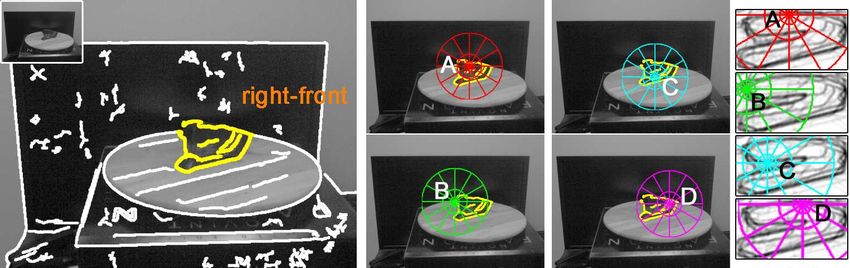
in Proc. 13th International Conference on Computer Vision (ICCV), Barcelona, Spain, 2011
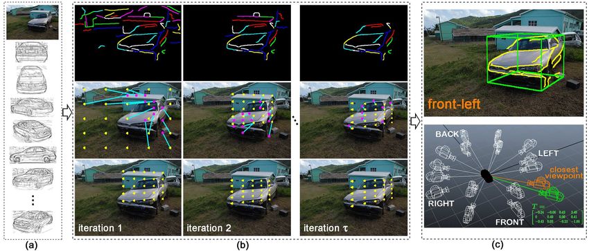
Figure 3. Iterative matching of BOBs in the image and the shape templates. Top: Estimated boundaries, and 3D BOBs that are matched to
the image BOBs. Middle and Bottom: Initially, the matches are established with multiple templates. After a few iterations, the matching
identifies the correct shape template, and the image contours selected as foreground indeed fall on the object. Corresponding pairs of image
and template BOBs are marked with the same color.
sample a total of 400 BOBs qj ∈ M. A shape context de- pixels, which is more precise. We count as true positives
scriptor Sj is associated with each qj , with a radius equal to the detected contour pixels that intersect with the object’s
3
10 of the object size. This way, each descriptor represents mask. The contours extracted originally form the total set
a significant part of the object, and there is a large overlap of true positives and true negatives.
between adjacent descriptors, see Fig. 3. Using the camera In addition to the 2D localization, the proposed approach
pose of each viewpoint, we can compute the 3D location of yields an estimate of the object’s 3D pose. For view-
each BOB qj . point classification, we take the viewpoint-label of the best
Testing. For each test image, we extract contours by matching template, whose camera centroid is the closest
the approach of [23]. We sample 121 BOBs pi on a uni- (Euclidean distance) to the estimated camera.
form 11x11 grid (empirically found optimal), and com- Evaluating our training setup. To determine how many
pute a shape context descriptor for every point pi . Ini- viewpoints are necessary to represent an object category, we
tially, the right scale for the descriptor is unknown. We train (a) 4, (b) 8, (c) 16, and (d) 32 shape templates for the
try multiple BOB radii, proportional to the image size, i.e. car category of the 3D object dataset [16]. The selected
radius = γ w+h 2 , with γ ∈ {0.05, 0.1, 0.15, 0.2}. We run
viewpoints are (a) front, left, back and right, height H1 ,
one iteration and keep the solution (F, T, X) that returns scale S1 , (b) all 8 viewpoints, height H1 , scale S1 , (c) all
the best score for the objective function in (7). In further 8 viewpoints, heights H1 , H2 , scale S1 , and (d) all 8 view-
iterations, the projection matrix T gives us an estimate of points, heights H1 , H2 , scales S1 , S2 . We test each setup on
the scale of the object. The radius of the descriptor is then the task of 8-viewpoint classification, and report the average
3 classification performance in Tab. 1.
set to 10 the size of the estimated object, to match the BOB
defined in the templates. This constitutes our default setup.
Evaluation criteria. To evaluate the 2D detection, we Number of templates 4 8 16 32
Average 64.5% 78.9% 85.4% 86.1%
use the standard PASCAL VOC detection quality criterion. performance ± 1.5% ± 0.7% ± 0.6% ± 0.5%
For a correct localization, the overlap ao between predicted Table 1. 3D object car dataset. Influence of the number of tem-
bounding box Bp and ground truth bounding box Bgt must plates on the pose estimation performance.
area(B ∩B )
exceed 50%, as defined by ao = area(Bpp ∪Bgt gt )
. Our 2D
localization is created by fitting a bounding box to the con- As expected, the performance improves as we add more
tours that are selected by our algorithm. Since our method templates. We choose to use 16 templates and not 32, be-
outputs contours, and not just a bounding box, we can com- cause the small performance gain does not justify the large
pute precision and recall of our detector in terms of contour increase in computation time. Our formulation is linear but
6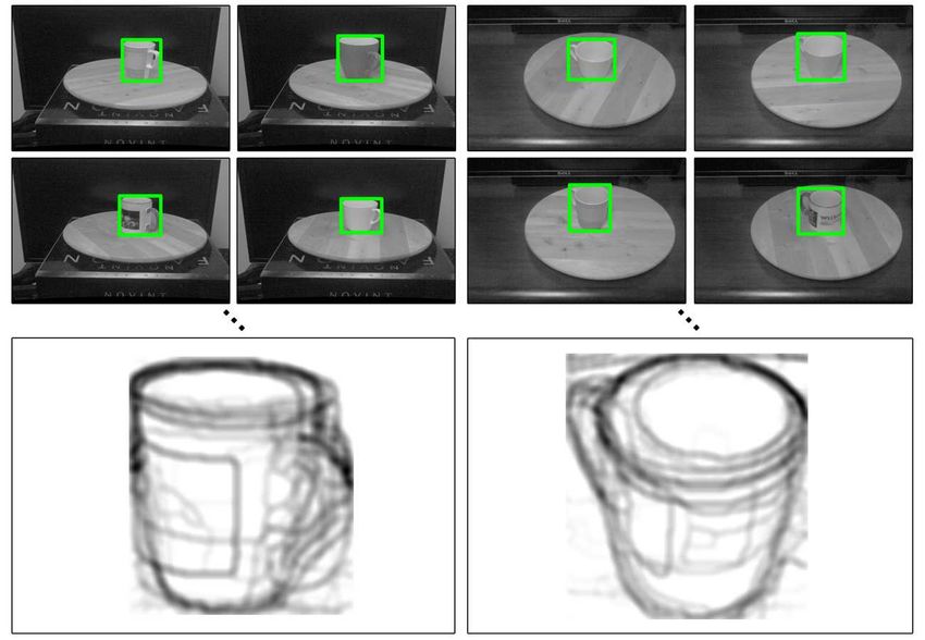
in Proc. 13th International Conference on Computer Vision (ICCV), Barcelona, Spain, 2011

the solver takes much longer to handle large matrices, which                 mate the equal error rate detection threshold teer . We run
makes it impractical to use 32 templates on large datasets.                  our mug detector on the remaining 207 images. Each can-
    Precision of pose estimation. To evaluate the preci-                     didate detection with an objective score below teer is clas-
sion of our camera pose estimate, we use synthetic data,                     sified as mug. The precision and recall at equal error rate
for which it is easy to obtain ground truth. We collect 6                    is measured at 84.3% ± 0.5%, which is better than the 59%
synthetic car models from free CAD databases, e.g. tur-                      reported in [23]. This also suggests that our shape templates
bosquid.com. Cameras are positioned at azimuth a =                           generalize well to other datasets.
0..360◦ in 10◦ steps, elevation e = 0..40◦ in 20◦ steps,
and distance d = 3, 5, 7 (generic units). 324 images are
rendered for each 3D model, for a total of 1944 test images
(see the supplemental material). For each image, we run
our car detector and record the 3D location of the estimated
camera. The position error is defined as the Euclidean dis-
tance between the centroids of ground truth camera and es-
timated camera. We measure an average error of 3.1 ± 1.2
units. There is a large variation because when we incor-
rectly estimate the camera, it is oftentimes because we have                 Figure 5. Our detection results on the PASCAL VOC 2006 car
mis-interpreted a viewpoint for its symmetric, e.g. front for                dataset (left) and the car show dataset (right).
back. The position error is also due to the underestima-
tion of the distance between object and camera, which is                         Fig. 6 shows our confusion matrices for viewpoint clas-
probably caused by our choice of resolving the scale via the                 sification, and compares our performance to that of [1, 19,
camera pose.                                                                 10, 18, 7] on different datasets. Our approach shows su-
    Independent viewpoints. We test a setup where one                        perior performance for nearly all viewpoints and categories
considers each viewpoint independently. We solve 16 in-                      relative to these approaches. After the deadline of camera-
dependent optimizations, as defined by (7), for each of the                  ready submissions, we became aware of the state-of-the-art
16 shape templates. The image receives the viewpoint-label                   results of viewpoint classification, presented in [6] – specif-
of the template that yields the best score. We here get a drop               ically, they reported the viewpoint classification accuracy of
in classification performance by 5.3% ± 0.4% compared to                     92.8% for cars, and 96.8% for bicycles. For the mice and
our default setup.                                                           staplers of the 3D object dataset, we achieve a viewpoint
    Qualitative results. Fig. 4 shows examples of success-                   classification of 78.2% ± 1.1%, resp. 77.6% ± 0.9%, and
ful detections and 3D object pose estimation. We success-                    improve by 3.2%, resp. 4.1% the results of [18].
fully detect the object boundaries, and we correctly esti-
mate the 3D poses. We are also able to identify interme-                     8. Conclusion
diate poses that are not available in our discrete set of shape
templates, e.g. the car in the lower-right image.                               We have presented a novel, shape-based approach to 3D
    Quantitative results. We first evaluate our performance                  pose estimation and view-invariant object detection. Shape,
on object detection. Fig. 5 shows the precision/recall of                    being one of the most categorical object features, has al-
                                                                             lowed us to formulate a new, sparse, view-centered ob-
our detector on the PASCAL cars and the car show dataset.
                                                                             ject representation in terms of a few, distinct, probabilistic,
We outperform the existing methods of [17, 11, 7, 13].                       shape templates. The templates are analogues to the well-
Our approach allows for non-rigid deformations and esti-                     known “mental images”, believed to play an important role
mates a full affine projection matrix, which explain our su-                 in human vision. We have formulated 3D object recognition
perior results. Our method can also detect object parts.                     as matching image contours to the set of shape templates.
We count 425 wheels in the car images of the 3D object                       To address the background clutter, we have lifted shape
dataset, and record precision/recall at equal error rate (EER)               matching from considering individual contours to match-
of 63.7% ± 0.5% for the wheel parts. Also, for the con-                      ing of new, mid-level features, called bags of boundaries
tour pixels detection, we measure precision/recall at EER                    (BOBs). BOBs are histograms of the right contours esti-
of 68.3% ± 0.2% on the 3D object car dataset. After the                      mated to belong to the foreground. In inference, BOBs in
deadline of camera-ready submissions, we became aware                        the image are iteratively re-located to jointly best summa-
                                                                             rize object boundaries and match them to the shape tem-
of competitive detection results, presented in [6] – specif-
                                                                             plates, while accounting for likely non-rigid shape defor-
ically, they reported an ROC curve that saturates at about                   mations. Our experiments have demonstrated that BOBs
60% recall.                                                                  are rich contextual features that facilitate view-invariant in-
    On the ETHZ Shape dataset, we use 24 positive mug im-                    ference, yielding favorable performance relative to the state
ages and 24 negative images from the other classes to esti-                  of the art on benchmark datasets.

                                                                         7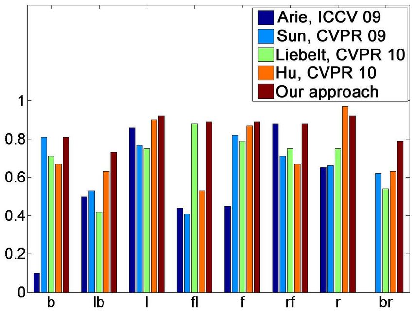
in Proc. 13th International Conference on Computer Vision (ICCV), Barcelona, Spain, 2011

Figure 4. Examples of our contour detection and 3D object pose estimation. Upper left: 3D object car dataset. Upper right: Table Top
stapler dataset. Lower left: ETHZ dataset. Lower right: car show dataset. We are successfully detecting the contours of the objects, and
we correctly estimate their 3D pose. The viewpoint label of the best matching template is taken as a discrete estimate of object pose, e.g.
right-front for the stapler. Example matches between image and shape templates BOBs are also shown. (Best viewed in color.)

                                                                                  visual recognition. Cog. Psych., 20(1):38–64, 1988.
                                                                              [4] S. J. Dickinson, R. Bergevin, I. Biederman, J.-O. Eklundh,
                                                                                  R. Munck-Fairwood, A. K. Jain, and A. Pentland. Panel re-
                                                                                  port: the potential of geons for generic 3-D object recogni-
                                                                                  tion. Image and Vision Computing, 15(4):277–292, 1997.
                                                                              [5] V. Ferrari, T. Tuytelaars, and L. Van Gool. Object detection
                                                                                  by contour segment networks. In ECCV, 2006.
                                                                              [6] C. Gu and X. Ren. Discriminative mixture-of-templates for
                                                                                  viewpoint classification. In ECCV, 2010.
                                                                              [7] W. Hu and S.-C. Zhu. Learning a probabilistic model mixing
                                                                                  3D and 2D primitives for view invariant object recognition.
                                                                                  In CVPR, 2010.
                                                                              [8] H. Jiang and S. X. Yu. Linear solution to scale and rotation
                                                                                  invariant object matching. In CVPR, 2009.
                                                                              [9] H. Li, E. Kim, X. Huang, and L. He. Object matching with
                                                                                  a locally affine-invariant constraint. In CVPR, 2010.
                                                                             [10] J. Liebelt and C. Schmid. Multi-view object class detection
                                                                                  with a 3D geometric model. In CVPR, 2010.
                                                                             [11] J. Liebelt, C. Schmid, and K. Schertler.          Viewpoint-
                                                                                  independent object class detection using 3D feature maps.
                                                                                  In CVPR, 2008.
                                                                             [12] A. Nemirovski. Sums of random symmetric matrices and
                                                                                  quadratic optimization under orthogonality constraints. In
                                                                                  Mathematical Programming, 2007.
                                                                             [13] M. Ozuysal, V. Lepetit, and P. Fua. Pose estimation for cate-
Figure 6. Viewpoint classification results. Top: cars in the 3D ob-               gory specific multiview object localization. In CVPR, 2009.
ject dataset. Middle: bikes in the 3D object dataset. Bottom: mice-          [14] Z. W. Pylyshyn. Mental imagery: In search of a theory. Be-
staplers-mugs in the Table Top dataset. Left: confusion matrices.                 havioral and Brain Sciences, 25(2):157–182, 2002.
Right: diagonal elements of our confusion matrices are compared              [15] N. Razavi, J. Gall, and L. V. Gool. Backprojection revisited:
with the state of the art.                                                        Scalable multi-view object detection and similarity metrics
                                                                                  for detections. In ECCV, 2010.
References                                                                   [16] S. Savarese and L. Fei-Fei. 3D generic object categorization,
                                                                                  localization and pose estimation. In ICCV, 2007.
 [1] M. Arie-Nachimson and R. Basri. Constructing implicit 3D                [17] H. Su, M. Sun, L. Fei-Fei, and S. Savarese. Learning a dense
     shape models for pose estimation. In ICCV, 2009.                             multi-view representation for detection, viewpoint classifica-
 [2] S. Belongie, J. Malik, and J. Puzicha. Shape matching                        tion and synthesis of object categories. In ICCV, 2009.
     and object recognition using shape contexts. IEEE TPAMI,                [18] M. Sun, G. Bradski, B. Xu, and S. Savarese. Depth-encoded
     24(4):509–522, 2002.                                                         hough voting for joint object detection and shape recovery.
 [3] I. Biederman. Surface versus edge-based determinants of                      In ECCV, 2010.

                                                                         8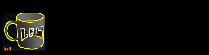
in Proc. 13th International Conference on Computer Vision (ICCV), Barcelona, Spain, 2011

[19] M. Sun, H. Su, S. Savarese, and L. Fei-Fei. A multi-view
     probabilistic model for 3d object classes. In CVPR, 2009.
[20] M. J. Tarr and I. Gauthier. Do viewpoint-dependent mech-
     anisms generalize across members of a class? Cognition,
     67(1-2):73–110, 1998.
[21] A. Thomas, V. Ferrari, B. Leibe, T. Tuytelaars, B. Schiel, and
     L. Van Gool. Towards multi-view object class detection. In
     CVPR, 2006.
[22] P. Yan, S. Khan, and M. Shah. 3D model based object class
     detection in an arbitrary view. In ICCV, 2007.
[23] Q. Zhu, L. Wang, Y. Wu, and J. Shi. Contour context se-
     lection for object detection: A set-to-set contour matching
     approach. In ECCV, 2008.

                                                                         9
You can also read