From metrology to digital data - Intelligent Embedded Systems

Advanced Research
                    Intelligent
                    Embedded
                    Systems

                                  From metrology to digital data

                                     Intelligence for Embedded Systems
                                                      Ph. D. and Master Course
                                                                  Manuel Roveri
                                                Politecnico di Milano, DEIB, Italy

Measure and measurements

§ The operation of measuring an unknown quantity xo
   can be modeled as taking an instance -or measurement-
   xi at time i with an ad-hoc sensor S
§ Even though S has been suitably designed and realized,
   the physical elements composing it are far from being
   ideal and introduce sources of uncertainty in the
   measurement process
§ As a consequence, xi represents only an estimate of xo

        This is a crucial point for the application
                   processing the data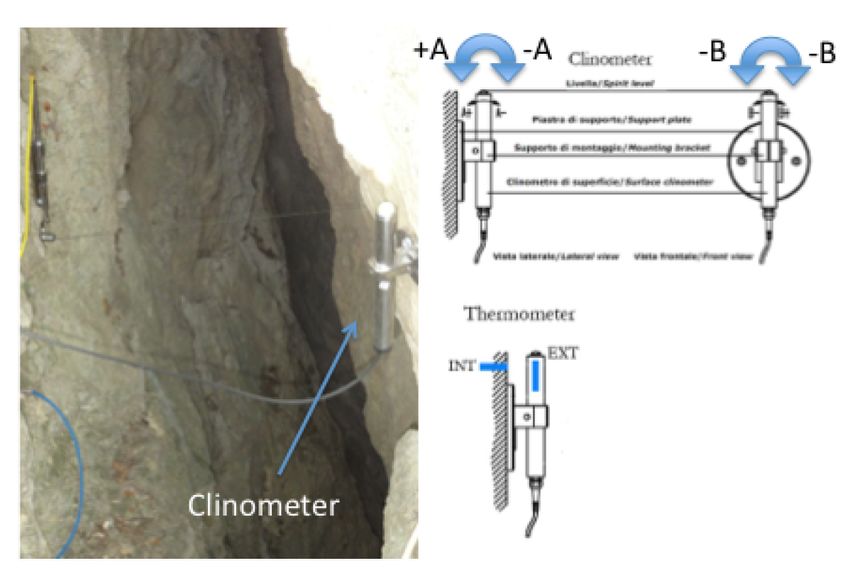

Environmental monitoring: rock collapse forecasting

                                        Towers
                                        of Rialba

Environmental monitoring: rock collapse forecasting

                                  Pluviometers
In addition:
Many temperature
sensors                                          High precision
                                                 inclinometers

                           Strain gauges

                                                 Mid precision
                                                 inclinometers

                                                 MEMS
                                                 accelerometer
                   Flow meters

Is xi an accurate and reliable estimate of x0 ?

§ Despite the formalization of the measurement process,
   several major aspects need to be investigated and
   addressed before claiming that a generic measurement xi
   is a an accurate and reliable estimate of xo.
§ For instance:
   • the sensor could be noisy;
   • the sensor or the processing electronics could be
     faulty;
   • the temperature could affect the sensor inducing bias in
     the measurements;
               How can we say that xi is an
           accurate and reliable estimate of x0 ?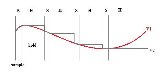

Some properties…

§ We would require subsequent measurements xi to be
   somehow centered around xo: an accurate sensor does
   not introduce some bias error (accuracy property).
§ Each measurement represents only an estimate of the
   true unknown value, the discrepancy between the two -
   or error- depends on the quality of the sensor and the
   working conditions under which the measure was taken
   (precision property).
§ We hope that the sensor is able to provide a long
   sequence of correct digits of the number associated
   with the acquired data (resolution property).

The measurement chain

     The functional chain representing the most common model
               describing a modern electronic sensor

The transducer: from x0 to xe

The transducer

§ A transducer is a device transforming a form of energy
   into another, here converting a physical quantity xo into
   an electric or electric-related quantity xe
§ E.g., a force transducer

Transducer (2)

§ Sensors can be active or passive in their transduction
   mechanism: an active sensor requires energy to carry out
   the operation and needs to be powered, whereas a
   passive sensor does not
      Required Energy to measure xe
§ Another relevant information is related to the time re-
   quested to produce a stable measurement. Such a
   time depends, for instance, on the dynamics of the
   transduction mechanisms or the time needed to complete
   the self calibration/compensation phase introduced to
   improve the quality of the sensor outcome.
      Required Time to measure xe

The conditioning circuit: from xe to xc

The conditioning circuit

§ The aim of the conditioning circuit is to provide an
   enhanced electrical quantity xc of xe.
§ Why do I need a conditioning circuit?
   ü the sensitivity of the sensor is amplified,

   ü the effect of the noise mitigated,

   ü the interval of definition of the electrical entity
     adapted to the requirements of the subsequent
     analog to digital converter.

The conditioning circuit (2)

§ What is the conditioning circuit?
   • It is an analog circuit juxtaposed to the transducer
     module
§ How does it work?
   • at first it usually amplifies xe

   • then, it filters its output (e.g., with a low pass filter) to
     improve the signal to noise ratio and the quality of
     the signal xc to be passed to the analog to digital
     conversion stage.

The conditioning circuit (3)

§ The conditioning circuit
   might also encompass a
   module designed to:
   • help compensating
     parasitic thermal effects,
     which influence the
     readout value
   • introduce corrections to
     linearize the relationship
     between the input xo
     and xc.                       Effect of the temperature on
                                          a strain gauge

ADC: from xc to xb (binary)

The analog to digital converter

§ The input to the module is the analog electrical signal
   xc and the output is a codeword xb represented in a
   binary format.
§ There is a large variety of architectures for ADCs, all of
   them having in common:
   • the sampling rate
   • the resolution (the number of bits of the codeword)

§ The conversion introduces an error associated with the
   quantization level, whose statistical properties may
   depend on the specific ADC architecture.

The analog to digital converter (2)

§ During the conversion phase, the input xc must be kept
   constant, operation carried out by the ”sample and hold”
   mechanism (the analog value is sampled and kept to
   avoid dangerous fluctuations in the input signal)

Sampling rates and resolution

             (3 bits per sample)
                                    100
Resolution

                                    011

                                    010

                                    001

                                           Sampling Period
                                   (Sampling Frequency, Spectrum Analysis,
                                    Maximum Frequency, Nyquist theorem)

Data Estimation: from xb to xi

The data estimation module (for smart sensors)

§ The final module (when present) introduces further
   corrections on xb by operating at the digital level.
§ In particular, it generally carries out a further calibration
   phase aiming at improving the quality of the final data xi
§ When a microprocessor is present to address the data
   estimation module needs, the sensor is defined to be a
   ”smart sensor”.
§ The microprocessor can carry out a more sophisticated
   processing relying on simple but effective algorithms,
   generally aimed at introducing corrections and
   structural error compensations.

Data Estimation Module:
 an example of smart clinometer sensor

                                    For instance, a thermal sensor
                                    can be onboard, in addition
                                    to the principal sensor, to
                                    compensate the thermal effect
                                    on the principal sensor readout.

The microprocessor carries
out the thermal compensation
by reading the temperature value,
comparing it with the rated
working temperature defined at
design time and introducing a
correction on the readout value

The data estimation module: averaging

§ When the dynamics of the signal are known not to
   change too quickly (compared with the time requested
   by the ADC to convert a value) or the signal is constant,
   the microcontroller can instruct the sensor to take a burst
   of n readings over time.
§ The outcome data sequence xb,j, j = 1,...,n can be used to
   provide an improved final estimate of xo by averaging

Now it’s time for a quick brainstorming…

Please, try to answer the following question:
how can all these uncertainties in the measurement
process affect the application/theory/technique I’m
studying or considering?

Abstracting the measurement chain …

        Create a model of the
       measurement process …

Modeling the measurement process:
the additive or “signal plus noise” model

§ The whole measurement process can now be seen as a
   black box, suitably described by an input-output model
   whose simplest, but generally effective form, is

                                                            Considered
                                                              Model

      where

                                         independent and identically
                                         distributed (i.i.d.) random variable

              The model implicitly assumes that the noise does
                    not depend on the working point xo

Modeling the measurement process:
the multiplicative model

§ Another common model for the sensor is the multiplicative
   one where

       In this way, the noise depends on the working point xo.
   In absolute terms, the impact of the noise on the signal is xoη,
     but the relative contribution is η and does not depend on xo

Now we have all the theoretical tools to define

1) Accuracy
2) Precision
3) Resolution

          These are crucial properties to
             assess the quality of a
             measurement process

1) Accuracy

§ We say that a measure is accurate when the expectation
   taken w.r.t. the noise satisfies

§ In order to have an accurate measurement, the instrument
   and the measurement process have not to introduce any
   bias contribution
                            bias term

Accuracy: how to remove the bias?

§ When the measurement process is biased we need to
   subtract the expected value (or its estimate) from the read
   value.
§ However, since k is unknown, we must rely on a reference
   value to estimate it
§ E.g., if we are able to drive the sensor to a controlled state
   where the expected value is known, say xo, then

               SENSOR CALIBRATION

Example: Sensor Calibration

§ We bought a low cost temperature sensor and are not
   sure about its accuracy. We wish to quantify the potential
   bias value so as to zero center subsequent measurements.
§ To this purpose, we drive our sensor to operate at a
   known reference value xo and wait until the dynamics
   effect associated with the change of state vanishes.
§ In the steady state the sensor shares the same temperature
   as the environment:

§ We iterate the process for different xo values to get a
   calibration curve

2) Precision

§ Under the signal plus noise framework, each taken
   measurement is seen as a realization of a random
   variable.
§ Measurements will then be spread around a given value
   (xo in the case of accurate sensors, xo + k in case of an
   inaccurate one), with the standard deviation defining a
   scattering level index
§ Precision is a measure of such scattering and is
   function of the standard deviation of the noise

Given a confidence level δ, precision defines an interval I for xo within
    which all values are indistinguishable due to the presence of
    uncertainty η: all values x ∈ I are equivalent estimates of xo

An example of precision: Gaussian Distribution

§ Gaussian distribution fη(0,ση2). The Gaussian hypothesis
   holds in many off-the-shelf integrated sensors
§ Under the Gaussian assumption and a confidence level δ,
   we have that a realization xi of xo lies in
   • I = [xo − 2ση , xo + 2ση ] with probability 0.95

   • I = [xo − 3ση , xo + 3ση ] with probability 0.997
§ The interval defines the precision (interval) of the measure
   at a given confidence δ.
§ For example, the precision of the sensor (sensor
   tolerance) could be defined as 3ση , so that x = xo ± 3ση

Precision: Unknown Distribution

§ When fη is unknown, we cannot use the strong results
   valid for the Gaussian distribution
§ In this case, we need to define an interval I function of δ
   within a pdf-free framework
§ The issue can be solved by invoking the Tchebychev
   theorem which, given a positive λ value and a confidence
   δ , grants the inequality

§ By selecting a wished confidence δ, e.g., δ = 0.95, we
   select the consequent value λ
§ The precision interval I is now x = xo ± λση

Precision: Unknown Distribution (2)

§ The lack of priors about the distribution is a cost we pay in
   terms of a larger tolerance interval

            By having a priori information about the noise
           distribution, the precision interval can be easily
                 characterized with a better precision

3) Resolution

§ Whereas precision is a property associated with a
   measure, resolution is associated with an instrument/
   sensor and represents the smallest value that can be
   perceived and differentiated by others given a
   confidence level
§ Example: if our instrument has a resolution of 1g, we will
   not be able to measure values of 1mg due to the limits of
   the instrument: the scale will make sense in steps of 1g
   (and all values in such interval will be equivalent and
   indistinguishable)
§ But …

Question

    Does a high resolution sensor imply
       high precision or accuracy?

    No, having a high resolution neither
    implies that the measure is accurate
                 nor precise

A real sensor example:
a temperature sensor for aquatic monitoring

§ The resolution of the instrument is high, but the impact of the noise
   on the readout value is high as well.
§ The sensor provides values within a [−4oC,36oC] interval with an
   additive error model influencing up to ±0.3.
§ We immediately derive that ση = 0.1 since the sensor is ruled by a
   Gaussian distribution from data-sheet information and
   we consider λ = 3

Last but not least…

§ Designing an embedded application for real-world
   applications requires to:
     identify the number of significant digits
        available within the given codeword
                   or (in other words)
   if the output of the data estimation module xi is
    represented by means of n bits, uncertainty is
                 affecting the readout,
    how many bits p are relevant out of the n?

A deterministic representation: noise-free data

§ The case covers the situation where acquired data are
   error-free and belong to the closed interval [a,b].
§ If n bits are made available to represent the data and no
   noise affects them, then each of the 2n available
   codewords are worth to be used
§ ∆ x between two subsequent data is
§ In this way the 2n code words are assigned as
               x1=a, x2=a+∆x , ... , x2n =b
§ Given a value xo, the maximum representation error is
   ∆x/2 and the average error is zero. If values are uniformly
   distributed in the interval [xo − ∆x/2 , xo + ∆x/2 ], then the
   variance of the error representation is ∆x2/12

A stochastic representation: noise-affected data

§ As we have seen in the measurement chain, data
   acquired from a sensor are noise-affected.
§ Obviously, we are not interested in spending bits to
   represent the noise when writing a number.
§ Precision introduces a constraint on the
   indistinguishable values we can acquire:
   • two data are distinguishable and deserve distinct
     codewords only if their distance is above the
     precision interval I which, as we have seen,
     depends on a predefined confidence level δ

A stochastic representation of noise-affected data

§ The number of independent values can be written as the
   ratio between the domain interval of the data and the
   value Im = 2λ ση of the probabilistic indistinguishability
   interval (ση being the uncertainty standard deviation
   associated with the measurement process)
§ The number of independent points Ip is
                                           The signal is bounded

                                            Interval introduced
                                              by the precision
§ The number of significant bits is

Example: the impact of a normally distributed noise

§ Figure shows how values around xo = 6 are affected by
   noise under the assumption that the noise is normal (zero
   mean, unitary standard deviation and λ = 3).

• Codewords are xo =
  0,6,12,18 but the error
  distribution is shown
  only in correspondence
  of codewords xo = 6 and
  xo = 12.
• Given the tails of the
  distribution, we might
  erroneously assign with
  probability 1 − δ a
  wrong codeword to a
  given value.

Unbounded signal: the signal to noise ratio (SNR)

§ Consider now the case where the signal is not bounded in
   deterministic terms
§ Measurements are modeled as instances drawn from
   a stationary -possibly unknown- pdf.
§ A probabilistic interval can be identified for xo whose
   probabilistic extremes are associated with λxσx, being
   σx the standard deviation of the signal and λx the term
   modulating the width of the interval, chosen to grab
   confidence level δ.

The signal to noise ratio (SNR) – cont.

§ In this case, the number of independent values Ip depends
   on the interval between two distinct codewords, which are
   distinguishable according to δ

§ By considering the same λs both for the noise and signal
   we define the Signal to Noise ratio (SNR)

The signal to noise ratio (SNR) – cont.

§ The SNR is pdf-free and applies to any distribution
   thanks to the Tchebychev inequality, provided that the
   same λ value is considered.
§ The number of relevant bits p of the binary codeword
   finally becomes

§ If p ≥ n, all bits present in xi are statistically relevant;
   otherwise, only p out of n are relevant and n − p are
   associated with noise

Let’s play with MATLAB

§ Download the examples related to Lecture 2
§ In the ZIP file:
   • Example 2_A.m
      − About the accuracy and the calibration of a sensor

   • Example 2_B.m
      − About the precision and Tchebychev inequality

   • Example 2_C.m
      − About the noise-free and the noise-affected representation of
        data