GeoChronR - an R package to model, analyze, and visualize age-uncertain data
←
→
Page content transcription
If your browser does not render page correctly, please read the page content below
Geochronology, 3, 149–169, 2021
https://doi.org/10.5194/gchron-3-149-2021
© Author(s) 2021. This work is distributed under
the Creative Commons Attribution 4.0 License.

geoChronR – an R package to model, analyze, and visualize
age-uncertain data
Nicholas P. McKay1 , Julien Emile-Geay2 , and Deborah Khider3
1 School of Earth and Sustainability, Northern Arizona University, Flagstaff, AZ, USA
2 Department  of Earth Sciences, University of Southern California, Los Angeles, CA, USA
3 Information Sciences Institute, University of Southern California, Marina del Rey, CA, USA

Correspondence: Nicholas P. McKay (nicholas.mckay@nau.edu)

Received: 11 August 2020 – Discussion started: 7 September 2020
Accepted: 10 December 2020 – Published: 12 March 2021

Abstract. Chronological uncertainty is a hallmark of the           termination, it is impossible to properly assess the extent to
paleoenvironmental sciences and geosciences. While many            which past changes occurred simultaneously across regions,
tools have been made available to researchers to quantify age      accurately estimate rates of change or the duration of abrupt
uncertainties suitable for various settings and assumptions,       events, or attribute causality – all of which limit our capac-
disparate tools and output formats often discourage integra-       ity to apply paleogeoscientific understanding to modern and
tive approaches. In addition, associated tasks like propagat-      future processes. The need for better solutions to both char-
ing age-model uncertainties to subsequent analyses, and vi-        acterize uncertainty, and to explicitly evaluate how age un-
sualizing the results, have received comparatively little at-      certainty impacts the interpretation of records of past climate,
tention in the literature and available software. Here, we de-     ecology or landscapes, has been long recognized (e.g., Noren
scribe geoChronR, an open-source R package to facilitate           et al., 2013; National Academies of Sciences, Engineering,
these tasks. geoChronR is built around an emerging data            and Medicine, 2020, and reference therein). In response
standard (Linked PaleoData, or LiPD) and offers access to          to this need, the paleoenvironmental sciences and geoscien-
four popular age-modeling techniques (Bacon, BChron, Ox-           tific communities have made substantial advances toward im-
Cal, BAM). The output of these models is used to conduct           proving geochronological accuracy by
ensemble data analysis, quantifying the impact of chrono-
logical uncertainties on common analyses like correlation,          1. improving analytical techniques that allow for more pre-
regression, principal component, and spectral analyses by re-          cise age determination on smaller and context-specific
peating the analysis across a large collection of plausible age        samples (e.g., Eggins et al., 2005; Santos et al., 2010;
models. We present five real-world use cases to illustrate how         Zander et al., 2020);
geoChronR may be used to facilitate these tasks, visualize
the results in intuitive ways, and store the results for further    2. refining our understanding of how past changes in
analysis, promoting transparency and reusability.                      the Earth system impact chronostratigraphy, for exam-
                                                                       ple, improvements to the radiocarbon calibration curve
                                                                       (Reimer et al., 2011, 2013, 2020) and advances in our
                                                                       understanding of spatial variability in cosmogenic pro-
1     Introduction
                                                                       duction rates used in exposure dating (Balco et al.,
1.1    Background                                                      2009; Masarik and Beer, 2009; Charreau et al., 2019);
                                                                       and
Quantifying chronological uncertainties, and how they in-
fluence the understanding of past changes in Earth systems,         3. dramatically improving the level of sophistication and
is a unique and fundamental challenge of the paleoenviron-             realism in age–depth models used to estimate the ages
mental sciences and geosciences. Without robust error de-              of sequences between dated samples (e.g., Parnell et al.,

Published by Copernicus Publications on behalf of the European Geosciences Union.
150                                                                                N. P. McKay et al.: The geoChronR package

      2008; Bronk Ramsey, 2009; Blaauw, 2010; Blaauw and              2. For studies of new and individual records, few tools for
      Christen, 2011).                                                   ensemble analysis are available, and those that are re-
                                                                         quire a degree of comfort with coding languages and
   Over the past 20 years, these advances have been widely,              scientific programming that is rare among paleoenviron-
but not completely, adopted. Indeed, despite the progress                mental scientists and geoscientists.
made in quantifying uncertainty in both age determinations
and age models, comparatively few studies have formally               3. There is a disconnect between age-model develop-
evaluated how chronological uncertainty may have affected                ment and time-uncertain analysis. Published approaches
the inferences made from them. For instance, whereas the al-             have utilized either simplified age-modeling approaches
gorithms mentioned above have been broadly used, studies                 (e.g., Haam and Huybers, 2010; Routson et al., 2019) or
typically calculate a single “best” estimate (often the poste-           specialized approaches not used elsewhere in the com-
rior median or mean), use this model to place measured pa-               munity (e.g., Marcott et al., 2013; Tierney et al., 2013).
leoclimatic or paleoenvironmental data on a timescale, and              Extracting the relevant data from commonly used age-
then proceed to analyze the record with little to no reference       modeling algorithms, creating time-uncertain ensembles,
to the uncertainties generated as part of the age-modeling           then reformatting those data for analysis in available tools
exercise, however rigorous in its own right. In addition,            typically requires the development of extensive custom
few studies have evaluated sensitivity to the choice of age-         codes. geoChronR presents an integrative approach to facili-
modeling technique or choice of parameters, so that the typ-         tate this work.
ical discussion of chronological uncertainties remains partial
and qualitative.
                                                                     1.2   Design principles
   This paradigm is beginning to change. The vast major-
ity of modern age-uncertainty quantification techniques es-          geoChronR was built to lower the barriers to broader adop-
timate uncertainties by generating an “ensemble” of plausi-          tion of these emerging methods. Thus far, geoChronR has
ble age models, hundreds or thousands of plausible alternate         been primarily designed with Quaternary datasets in mind,
age–depth relationships that are consistent with radiometric         for which a variety of chronostratigraphic methods are avail-
age estimates, the depositional or accumulation processes of         able: radiometric dating (14 C, 210 Pb, U/Th), exposure dating,
the archive, and the associated uncertainties. In recent years,      layer counting, flow models (for ice cores), orbital alignment,
some studies have taken advantage of these age ensembles,            and more. Nevertheless, the primary uncertainty quantifica-
evaluating how the results of their analyses and conclusions         tion device is age ensembles, regardless of how they were
vary across the ensemble members (e.g., Blaauw et al., 2007;         produced. As such, geoChronR’s philosophy and methods
Parnell et al., 2008; Blaauw, 2012; Khider et al., 2014, 2017;       can be broadly applicable to any dataset for which age en-
Bhattacharya and Coats, 2020). By applying an analysis to all        sembles can be generated.
members of an age ensemble, the impact of age uncertainties             geoChronR provides an easily accessible, open-source,
on the conclusion of a study may be formally evaluated.              and extensible software package of industry-standard and
   Despite its potential to substantially improve uncertainty        cutting-edge tools that provides users with a single environ-
quantification for the paleoenvironmental sciences and geo-          ment to create, analyze, and visualize time-uncertain data.
sciences, this framework is not widely utilized. The majority        geoChronR is designed around emerging standards that con-
of studies utilizing this approach have been regional (e.g.,         nect users to growing libraries of standardized datasets for-
Tierney et al., 2013; Khider et al., 2017; Deininger et al.,         matted in the Linked PaleoData (LiPD) format (McKay
2017; McKay et al., 2018; Bhattacharya and Coats, 2020) or           and Emile-Geay, 2016), including thousands of datasets
global-scale (e.g., Shakun et al., 2012; Marcott et al., 2013;       archived at the World Data Service for Paleoclimatology
Kaufman et al., 2020a) syntheses. Some primary publica-              (WDS-Paleo) and lipdverse.org, those at the LinkedEarth
tions of new records incorporate time-uncertain analysis into        wiki (http://wiki.linked.earth, last access: 22 February 2021),
their studies (e.g., Khider et al., 2014; Boldt et al., 2015; Fal-   and Neotoma (Williams et al., 2018) via the neotoma2lipd
ster et al., 2018), but this remains rare. We suggest that there     package (McKay, 2020). Furthermore, several utilities ex-
are several reasons for the lack of adoption of these tech-          isting to convert or create datasets in the LiPD format.
niques:                                                              The most user-friendly and widely used platform to cre-
                                                                     ate LiPD datasets is the “LiPD Playground” (http://lipd.net/
  1. For synthesis studies, the necessary geochronological           playground, last access: 22 February 2021), a web-based
     data are not publicly available for the vast majority           platform that guides users through the process of format-
     of records. Even when they are available, the data are          ting LiPD datasets. For the conversion of large collections of
     archived in diverse and unstructured formats. Together,         data, a variety of useful tools are available in R, Python, and
     this makes what should be a simple process of aggre-            MATLAB as part of the LiPD utilities (https://github.com/
     gating and preparing data for analysis prohibitively time       nickmckay/lipd-utilities, last access: 22 February 2021), in-
     consuming.                                                      cluding an Excel-template converter in Python. geoChronR

Geochronology, 3, 149–169, 2021                                                      https://doi.org/10.5194/gchron-3-149-2021
N. P. McKay et al.: The geoChronR package                                                                                   151

reuses existing community packages, for which it provides         of these algorithms through their R packages (Parnell et al.,
a standardized interface, with LiPD as input/output format.       2008; Blaauw et al., 2020; Martin et al., 2018), standardiz-
Central to the development of the code and documentation          ing and streamlining the input and the extraction of the age
were two workshops carried out in 2016 and 2017 at North-         ensembles from the MCMC results for further analysis.
ern Arizona University, gathering a total of 33 participants.        In addition to working with ensembles from tie-point age
The workshop participants were predominantly early career         models, geoChronR connects users to probabilistic models of
researchers with > 50 % participation of women, who are           layer-counted chronologies. The banded age model (BAM)
underrepresented in the geosciences. Exit surveys were con-       (Comboul et al., 2014) was designed to probabilistically
ducted to gather feedback and to suggest improvements and         simulate counting uncertainty in banded archives, such as
extensions, which were integrated into subsequent versions        corals, ice cores, or varved sediments, but can be used to
of the software.                                                  crudely simulate age uncertainty for any record and is useful
                                                                  when the data or metadata required to calculate an age–depth
1.3    Outline of the paper                                       model are unavailable (e.g., Kaufman et al., 2020a). Here, we
                                                                  briefly describe the theoretical basis and applications of each
This paper describes the design, analytical underpinnings,        of the four approaches integrated in geoChronR.
and most common use cases of geoChronR. Section 2 de-
scribes the integration of age-modeling algorithms with
                                                                  2.1   Bacon
geoChronR. Section 3 details the methods implemented for
age-uncertainty analysis. Section 4 goes through the princi-      The Bayesian ACcumulatiON (Bacon) algorithm (Blaauw
ples and implementation of age-uncertain data visualization       and Christen, 2011) is one of the most broadly used age-
in geoChronR, and Sect. 5 provides five real-world examples       modeling techniques and was designed to take advantage
of how geoChronR can be used for scientific workflows.            of prior knowledge about the distribution and autocorrela-
                                                                  tion structure of sedimentation rates in a sequence to better
2     Age-uncertainty quantification in geoChronR                 quantify uncertainty between dated levels. Bacon divides a
                                                                  sediment sequence into a parameterized number of equally
geoChronR does not introduce any new approaches to                thick segments; most models use dozens to hundreds of these
age-uncertainty quantification; rather, it integrates existing,   segments. Bacon then models sediment deposition, with uni-
widely used packages while streamlining the acquisition of        form accumulation within each segment, as an autoregressive
age ensemble members. Fundamentally, there are two types          gamma process, where both the amount of autocorrelation
of age models used in the paleoenvironmental sciences and         and the shape of the gamma distribution are given prior esti-
geosciences: tie-point and layer-counted models. Most of          mates. The algorithm employs an adaptive MCMC algorithm
the effort in age-uncertainty quantification in the commu-        that allows for Bayesian learning to update these variables
nity has been focused on tie-point modeling, where the goal       given the age–depth constraints and converge on a distribu-
is to estimate ages (and their uncertainties) along a depth       tion of age estimates for each segment in the model. Bacon
profile given chronological estimates (and their uncertain-       has two key parameters: the shape of the accumulation prior
ties) at multiple depths downcore. Over the past 20 years,        and the segment length, which can interact in complicated
these algorithms have progressed from linear or polyno-           ways (Trachsel and Telford, 2017). In our experience, the
mial regressions with simple characterizations of uncer-          segment length parameter has the greatest impact on the ul-
tainty (Heegaard et al., 2005; Blaauw, 2010) to more rig-         timate shape and amount of uncertainty simulated by Bacon,
orous techniques, particularly Bayesian approaches: as of         as larger segments result in increased flexibility of the age–
writing, the three most widely used algorithms are Bacon          depth curve and increased uncertainty between dated levels.
(Blaauw and Christen, 2011), BChron (Parnell et al., 2008),       Bacon is written in C++ and R, with an R interface. More
and OxCal (Bronk Ramsey, 2008), which are all Bayesian            recently, the authors released an R package called “rbacon”
age-deposition models that estimate posterior distributions       (Blaauw et al., 2020), which geoChronR leverages to pro-
on age–depth relationships using different assumptions and        vide access to the algorithm. Bacon will optionally return a
methodologies. Trachsel and Telford (2017) reviewed the           thinned subset of the stabilized MCMC accumulation rate
performance of these three algorithms, as well as a non-          ensemble members, which geoChronR uses to form age en-
Bayesian approach (Blaauw, 2010), and found that the three        semble members for subsequent analysis.
Bayesian approaches generally outperform previous algo-
rithms, especially when appropriate parameters are chosen         2.2   BChron
(although choosing appropriate parameters can be challeng-
ing). Bacon, BChron, and OxCal all leverage Markov chain          BChron (Haslett and Parnell, 2008; Parnell et al., 2008) uses
Monte Carlo (MCMC) techniques to sample the posterior             a similar approach, using a continuous Markov monotone
distributions, thereby quantifying age uncertainties as a func-   stochastic process coupled to a piecewise linear deposition
tion of depth in the section. geoChronR interfaces with each      model. This simplicity allows semi-analytical solutions that

https://doi.org/10.5194/gchron-3-149-2021                                                  Geochronology, 3, 149–169, 2021
152                                                                              N. P. McKay et al.: The geoChronR package

make BChron computationally efficient. BChron was origi-           to be treated as a variable, and the model will estimate the
nally intended to model radiocarbon-based age–depth mod-           most likely values of k given a prior estimate and the data.
els in lake sedimentary cores of primarily Holocene age, but       The downside of this flexibility is that this calculation can
its design allows broader applications. In particular, model-      greatly increase the convergence time of the model. OxCal is
ing accumulation as additive independent gamma increments          written in C++, with an interface in R (Martin et al., 2018).
is appealing for the representation of hiatuses, particularly      OxCal does not typically calculate posterior ensembles for a
for speleothem records, where accumulation rate can vary           depth sequence but can optionally output MCMC posteriors
quite abruptly between quiescent intervals of near-constant        at specified levels in the sequence. geoChronR uses this fea-
accumulation (Parnell et al., 2011; Dee et al., 2015; Hu et al.,   ture to extract ensemble members for subsequent analysis.
2017). The downside of this assumption is that BChron is
known to exaggerate age uncertainties in cases where sedi-         2.4   BAM
mentation varies smoothly (Trachsel and Telford, 2017).
   Bchron has several key parameters which allow a user            BAM (Comboul et al., 2014) is a probabilistic model of age
to encode their specific knowledge about their data. In par-       errors in layer-counted chronologies. The model allows a
ticular, the outlierProbs parameter is useful in giving            flexible parametric representation of such errors (either as
less weight to chronological tie points that may be consid-        Poisson or Bernoulli processes) and separately considers the
ered outliers, either because they create a reversal in the        possibility of double counting or missing a band. The model
stratigraphic sequence, or because they were flagged dur-          is parameterized in terms of the error rates associated with
ing analysis (e.g., contamination). This is extremely use-         each event, which are intuitive parameters to geoscientists,
ful for radiocarbon-based chronologies where the top age           and may be estimated via replication (DeLong et al., 2013).
may not be accurately measured for modern samples. The             In cases where such rates can be estimated from the data
thetaMhSd, psiMhSd, and muMhSd parameters control                  alone, an optimization principle may be used to identify a
the Metropolis–Hastings standard deviation for the age pa-         more likely age model when a high-frequency common sig-
rameters and compound Poisson gamma scale and mean, re-            nal can be used as a clock (Comboul et al., 2014). As of now,
spectively, which influence the width of the ensemble be-          BAM does not consider uncertainties about such parameters,
tween age control tie points. geoChronR uses the same de-          representing a weakness of the method. Bayesian generaliza-
fault values as the official Bchron package, and we recom-         tions have been proposed (Boers et al., 2017), which could
mend that users only change them if they have good cause           one day be incorporated into geoChronR if the code is made
for doing so.                                                      public. BAM was coded in MATLAB, Python, and R, and it
                                                                   is this latter version that geoChronR uses.

2.3   OxCal
                                                                   2.5   Data storage
The OxCal software package has a long history and ex-
                                                                   geoChronR archives the outcome of all of these models in
tensive tools for the statistical treatment of radiocarbon
                                                                   the LiPD format (McKay and Emile-Geay, 2016). One of the
and other geochronological data (Bronk Ramsey, 1995).
                                                                   primary motivations for LiPD was to facilitate age-uncertain
In Bronk Ramsey (2008), age–depth modeling was intro-
                                                                   analysis, and geoChronR is designed to leverage these capa-
duced with three options for modeling depositional pro-
                                                                   bilities. LiPD can store multiple chronologies (called “chron-
cesses that are typically useful for sedimentary sequences:
                                                                   Data” in LiPD), each of which can contain multiple mea-
uniform, varve, and Poisson deposition models, labeled
                                                                   surement tables (which house the measured chronological
the U-sequence, V-sequence and P-sequence models, re-
                                                                   constraints) and any number of chronological models (which
spectively. The Poisson-based model is the most broadly
                                                                   comprise both the results produced of the analysis, as well
applicable for sedimentary or other accumulation-based
                                                                   as metadata about the method used to produce those results)
archives (e.g., speleothems), and although any sequence
                                                                   (Fig. 1). In LiPD, chronological models include up to three
type can be used in geoChronR, most users should use
                                                                   types of tables:
a P sequence, which is the default. Analogously to seg-
ment length parameter in Bacon, the k parameter (called             1. ensemble tables, which store the output of an algorithm
eventsPerUnitLength in geoChronR) controls how                         that produces age-model ensembles, and a reference
many events are simulated per unit of depth and has a strong           column (typically depth);
impact on the flexibility of the model, as well as the ampli-
                                                                    2. summary tables, which describe summary statistics pro-
tude of the resulting uncertainty. As the number of events
                                                                       duced by the algorithm (e.g., median and 2σ uncertainty
increases, the flexibility of the model, and the uncertainties,
                                                                       ranges); and
decreases. Trachsel and Telford (2017) found that this pa-
rameter has a large impact on the accuracy of the model,            3. distribution tables, which store age–probability distri-
more so than the choices made in Bacon or Bchron. Fortu-               butions for calibrated ages, typically only used for cali-
nately, Bronk Ramsey et al. (2010) made it possible for k              brated radiocarbon ages.

Geochronology, 3, 149–169, 2021                                                    https://doi.org/10.5194/gchron-3-149-2021
N. P. McKay et al.: The geoChronR package                                                                                          153

                                                                        tionally, ensembles of climate proxy or paleoenvironmental
                                                                        data) to propagate uncertainties through all steps of an anal-
                                                                        ysis. Effectively, this is done by randomly sampling ensem-
                                                                        ble members and then repeating the analysis many (typically
                                                                        hundreds to thousands) times, each time treating a different
                                                                        ensemble member as a plausible realization. This builds an
                                                                        output ensemble that quantifies the impact of those uncer-
                                                                        tainties on a particular inference. These output ensembles
                                                                        rarely lend themselves to binary significance tests (e.g., a
                                                                        p value below 0.05) but are readily used to estimate prob-
                                                                        ability densities or quantiles, and thus they provide quantita-
                                                                        tive evidence about which results are robust to age and proxy
                                                                        uncertainty (and which are not). Version 1.0.0 of geoChronR
                                                                        implemented ensemble analytical techniques for four of the
                                                                        most common analyses in the paleoenvironmental sciences
                                                                        and geosciences: correlation, regression, spectral, and prin-
                                                                        cipal component analyses.

                                                                        3.1   Correlation

                                                                        Correlation is the most common measure of a relation-
                                                                        ship between two variables (X and Y ). Its computation is
                                                                        fast, lending itself to ensemble analysis, with a handful of
                                                                        pretreatment and significance considerations that are rele-
                                                                        vant for ensembles of paleoenvironmental and geoscientific
                                                                        data. geoChronR implements three methods for correlation
                                                                        analysis: Pearson’s product moment, Spearman’s rank, and
Figure 1. Schematic representation of a Linked PaleoData (LiPD)         Kendall’s tau. Pearson correlation is the most common cor-
dataset, with a focus on chronological data. A LiPD dataset can con-    relation statistic but assumes normally distributed data. This
tain one or more instances of all of the data objects and structures.   assumption is commonly not met in paleoenvironmental or
The PaleoData structure mirrors that of the chronData but is not
                                                                        geoscientific datasets but can be can be overcome by map-
shown for clarity.
                                                                        ping both datasets to a standard normal distribution prior to
                                                                        analysis (Emile-Geay and Tingley, 2016; van Albada and
                                                                        Robinson, 2007). Alternatively, the Spearman and Kendall
   LiPD can also store relevant metadata about the modeling
                                                                        correlation methods are rank based and do not require nor-
exercise, including the values of the parameters used to gen-
                                                                        mally distributed input data, and they are useful alternatives
erate the data tables. This storage mechanism allows for an
                                                                        in many applications.
efficient sweep over the function parameters and comparison
                                                                           All correlation analyses for time series are built on the
of the results.
                                                                        assumption the datasets can be aligned on a common time-
   The capability of geoChronR to structure the output of the
                                                                        line. Age-uncertain data violate this assumption. We over-
popular age-modeling algorithms described in this section
                                                                        come this by treating each ensemble member from one or
into LiPD is a key value proposition of geoChronR. Once
                                                                        more age-uncertainty time series as valid for that iteration,
structured as a LiPD object in R, these data and models can
                                                                        then “bin” each of the time series into coeval intervals. The
be written out to a LiPD file and readily analyzed, shared,
                                                                        “binning” procedure in geoChronR sets up an interval, which
and publicly archived.
                                                                        is typical evenly spaced, over which the data are averaged.
                                                                        Generally, this intentionally degrades the median resolution
3   Age-uncertain data analysis in geoChronR                            of the time series, for example, a time series with 37-year
                                                                        median spacing could be reasonably “binned” into 100- or
Some theoretical work has attempted to quantify how                     200-year bins. The binning procedure is repeated for each en-
chronological uncertainty may affect various paleoenviron-              semble member, meaning that between different ensembles,
mental and geoscientific inferences (e.g., Huybers and Wun-             different observations will be placed in different bins.
sch, 2004); however, such efforts are hard to generalize given             Following binning, the correlation is calculated and
the variety of age-uncertainty structures in real-world data.           recorded for each ensemble member. The standard way to as-
Consequently, geoChronR follows a general, pragmatic, and               sess correlation significance is using a Student’s t test, which
broadly used approach that leverages age ensembles (and op-             assumes normality and independence. Although geoChronR

https://doi.org/10.5194/gchron-3-149-2021                                                         Geochronology, 3, 149–169, 2021
154                                                                             N. P. McKay et al.: The geoChronR package

can overcome the normality requirement, as discussed above,       in R by Ventura et al. (2004). FDR explicitly controls for
paleoenvironmental time series are often highly autocorre-        spurious discoveries arising from repeatedly carrying out the
lated and not serially independent, leading to spurious assess-   same test. At a 5 % level, one would expect a 1000-member
ments of significance (Hu et al., 2017). geoChronR addresses      ensemble to contain 50 spurious “discoveries” – instances
this potential bias using three approaches:                       of the null hypothesis (here “no correlation”) being rejected.
                                                                  FDR takes this effect into account to minimize the risk of
 1. The simplest approach is to adjust the test’s sample          identifying such spurious correlations merely on account of
    size to reflect the reduction in degrees of freedom           repeated testing. In effect, it filters the set of “significant”
    due to autocorrelation. Following Dawdy and Matalas           results identified by each hypothesis test (effective N, isop-
    (1964), the effective number of degrees of freedom is         ersistent, or isospectral).
           1−φ φ1,X
    ν = n 1+φ1,X
              1,X φ1,X
                       , where n is the sample size (here, the
    number of bins) and where φ1,X , φ1,X are the lag-1 au-
                                                                  3.2   Regression
    tocorrelation of two time series (X and Y , respectively).
    This approach is called “effective n” in geoChronR. It is     Linear regression is a commonly used tool to model the re-
    an extremely simple approach, with no added computa-          lationships between paleoenvironmental data and instrumen-
    tions by virtue of being a parametric test using a known      tal or other datasets. One application is calibration in time
    distribution (t distribution). A downside is that the cor-    (Grosjean et al., 2009), whereby a proxy time series is cal-
    rection is approximate and can substantially reduce the       ibrated to an instrumental series with an linear regression
    degrees of freedom (Hu et al., 2017) to less than 1 in        model over their period of overlap. This approach is par-
    cases of high autocorrelation, which is common in pa-         ticularly vulnerable to age uncertainties, as both the devel-
    leoenvironmental time series. This may result in overly       opment of the relationship and the reconstruction are af-
    conservative assessment of significance, so this option       fected. geoChronR propagates age (and optionally proxy)
    is therefore not recommended.                                 uncertainties through both the fitting of the ordinary least
                                                                  squares regression model and the reconstruction “forecast”
 2. A parametric alternative is to generate surrogates, or
                                                                  using the ensemble model results and age uncertainty. In
    random synthetic time series, that emulate the persis-
                                                                  the calibration-in-time use cases, ordinary linear regression,
    tence characteristics of the series. This “isopersistent”
                                                                  which only considers uncertainty in Y is appropriate, as un-
    test generates M (say, 500) simulations from an autore-
                                                                  certainty in the time axis is estimated from the ensemble.
    gressive process of order 1 (AR(1)), which has been fit-
                                                                  Like the correlation algorithm, ensemble regression uses an
    ted to the data. These random time series are then used
                                                                  ensemble binning procedure that is analogous to correlation.
    to obtain the null distribution and compute p values,
                                                                  geoChronR then exports uncertainty structure of the modeled
    which therefore measure the probability that a correla-
                                                                  parameters (e.g., slope and intercept), as well as the ensem-
    tion as high as the one observed (ro ) could have arisen
                                                                  ble of reconstructed calibrated data through time. Although
    from correlating X or Y with AR(1) series with identi-
                                                                  calibration in time is the primary application of regression in
    cal persistence characteristics as the observations. This
                                                                  geoChronR, users should be aware that in other applications,
    approach is particularly suited if an AR model is a sensi-
                                                                  the use of ordinary linear regression may result in biases if
    ble approximation to the data, as is often the case (Ghil
                                                                  the uncertainties in X are not considered.
    et al., 2002). However, it may be overly permissive or
    overly conservative in some situations.
                                                                  3.3   Principal component analysis
 3. A non-parametric alternative is the approach of
    Ebisuzaki (1997), which generates surrogates by scram-        geoChronR implements the age-uncertain principal compo-
    bling the phases of X and Y , thus preserving their power     nent analysis (PCA) procedure introduced by Anchukaitis
    spectrum. To generate these “isospectral” surrogates,         and Tierney (2013), with some minor modifications and ad-
    geoChronR uses the make_surrogate_data func-                  ditions. Like correlation and regression, PCA (or empiri-
    tion from the rEDM package (Park et al., 2020). This          cal orthogonal function (EOF) analysis) requires temporally
    method makes the fewest assumptions as to the struc-          aligned observations, and geoChronR uses a binning proce-
    ture of the series, and its computational cost is moder-      dure to achieve this across multiple ensembles. This differs
    ate, making it the default in geoChronR.                      from the implementation of Anchukaitis and Tierney (2013),
                                                                  who interpolated the data to a common time step. In addition,
   In addition to the impact of autocorrelation on this analy-    traditional singular-value decomposition approaches to PCA
sis, repeating the test over multiple ensemble members raises     require a complete set of observations without any miss-
the issue of test multiplicity (Ventura et al., 2004), also       ing values. For paleoclimate data, especially when consider-
known as the “look elsewhere effect”. To overcome this prob-      ing age uncertainty, this requirement is often prohibitive. To
lem, we control for this false discovery rate (FDR) using the     overcome this, geoChronR implements multiple options for
simple approach of Benjamini and Hochberg (1995), coded           PCA using the pcaMethods package (Stacklies et al., 2007).

Geochronology, 3, 149–169, 2021                                                   https://doi.org/10.5194/gchron-3-149-2021
N. P. McKay et al.: The geoChronR package                                                                                    155

The default and most rigorously tested option is a proba-         Lisiecki, 2010), or characterizing the continuum of climate
bilistic PCA (PPCA) approach that uses expectation maxi-          variability (Huybers and Curry, 2006; Zhu et al., 2019). Yet,
mization algorithms to infill missing values (Roweis, 1998).      spectral analysis in the paleoenvironmental sciences and geo-
This algorithm assumes that the data and their uncertainties      sciences faces unique challenges: chronological uncertain-
are normally distributed, which is often (but not always) a       ties, of course, as well as uneven sampling, which both vio-
reasonable assumption for paleoenvironmental data. As in          late the assumptions of classical spectral methods (Ghil et al.,
the other analytical approaches in geoChronR, users can op-       2002). To facilitate the quantification of chronological un-
tionally transform each series to normality using the inverse     certainties in such assessments, geoChronR implements four
Rosenblatt transform (van Albada and Robinson, 2007). This        spectral approaches:
is the recommended, and the default, option but does not
                                                                      1. the Lomb–Scargle periodogram (VanderPlas, 2018),
guarantee that the uncertainties will be Gaussian. As in cor-
                                                                         which uses an inverse approach to the harmonic anal-
relation and regression, geoChronR propagates uncertainties
                                                                         ysis of unevenly spaced time series;
through the analysis by repeating the analysis across ran-
domly sampled age and/or proxy ensemble members to build              2. REDFIT, a version of the Lomb–Scargle periodogram
output ensembles of the loadings (eigenvectors), variance ex-            tailored to paleoclimatic data (Schulz and Mudelsee,
plained (eigenvalues), and principal component time series.              2002; Mudelsee, 2002; Mudelsee et al., 2009);
Because the sign of the loadings in PCAs is arbitrary and                geoChronR uses the implementation of REDFIT from
vulnerable to small changes in the input data, geoChronR                 the dplR package (Bunn, 2008);
reorients the sign of the loadings for all principal compo-
nents (PCs) so that the mean of the loadings is positive. For         3. the wavelet-based method of Mathias et al. (2004),
well-defined modes, this effectively orients ensemble PCs,               called “nuspectral”, which is a wavelet version the
but loading orientation may be uncertain for lower-order, or             Lomb–Scargle method, similar to the weighted wavelet
more uncertain, modes.                                                   Z-transform algorithm of Foster (1996), though it is
   As in Anchukaitis and Tierney (2013), we use a modified               prohibitively slow in this implementation, and the fast
version of Preisendorfer’s “Rule N” (Preisendorfer and Mob-              version using a compact-support approximations of the
ley, 1988) to estimate which modes include more variabil-                mother wavelet did not perform well in our tests; and
ity than those that can arise from random time series with            4. the multi-taper method (MTM) of Thomson (1982), a
comparable characteristics to the data. geoChronR uses a rig-            mainstay of spectral analysis (Ghil et al., 2002) de-
orous “red” noise null hypothesis, modified from Neumaier                signed for evenly spaced time series. geoChronR uses
and Schneider (2001), where following the selection of the               the MTM implementation of Meyers (2014), which cou-
age ensemble in each iterations, a synthetic autoregressive              ples MTM to efficient linear interpolation, together with
time series is simulated based on parameters fit from each               various utilities to define autoregressive and power-law
dataset. This means that the characteristics of the null time            benchmarks for spectral peaks.
series, including the temporal spacing, autocorrelation, and,
optionally, the first-order trend, match those of each dataset      As described in Sect. 3.1, mapping to a standard nor-
and vary between locations and ensemble iterations. For each      mal is applied by default to avoid strongly non-normal
iteration, the ensemble PCA procedure is replicated with the      datasets from violating the methods’ assumptions. This
synthetic null dataset, using the same age ensemble member        can be relaxed by setting gaussianize = FALSE in
randomly selected for the real data. This effectively propa-      computeSpectraEns.
gates the impact of age uncertainty into null hypothesis test-
ing. Following the analysis, the distribution of eigenvalues      4    Visualization with geoChronR
calculated by the ensemble PCA is typically compared with
the 95th percentile of the synthetic eigenvalue results in a      One of the challenges of ensembles is that they add
scree plot. Only modes whose eigenvalues exceed this thresh-      at least one additional dimension to the results, which
old should be considered robust.                                  can be difficult to visualize. geoChronR aims to facili-
                                                                  tate simple creation of intuitive, publication-quality figures
3.4   Spectral analysis
                                                                  that provide multiple options for visualizing the impacts
                                                                  of age uncertainty, while maintaining flexibility for users
Many research questions in paleoclimatology and related           to customize their results as needed. To meet the mul-
geosciences revolve around spectral analysis: describing          tiple constraints of simplicity, quality, and customization,
phase leads and lags among different climate system compo-        geoChronR relies heavily on the ggplot2 package (Wick-
nents over the Pleistocene (e.g., Imbrie et al., 1984; Lisiecki   ham, 2016). High-level plotting functions in geoChronR
and Raymo, 2005; Khider et al., 2017), the hunt for astro-        (e.g., plotTimeseriesEnsRibbons and plotPca)
nomical cycles over the Holocene (Bond et al., 2001) or in        produce complete figures as ggplot2 objects, which can be
deep time (Meyers and Sageman, 2007; Meyers, 2012, 2015;          readily customized by adding or changing ggplot2 layers.

https://doi.org/10.5194/gchron-3-149-2021                                                    Geochronology, 3, 149–169, 2021
156                                                                             N. P. McKay et al.: The geoChronR package

   The figures in Sect. 5 are all produced by geoChronR and       this reference frame. geoChronR implements this conven-
generally fall into three categories: time series, mapping, and   tion by default, although the scales can be readily mod-
spectra. The default graphical mode is used throughout the        ified using ggplot2. In addition, the abscissa (log10 f )
figures of this paper; this aesthetic is what geoChronR pro-      is labeled according to the corresponding period, which is
duces by default but is readily modified by the user as de-       more intuitive than frequency to scientists reading the plot.
sired.                                                            To help identify significant periodicities, confidence limits
                                                                  can be superimposed, based on user-specified benchmarks
4.1   Time series
                                                                  (see Sect. 5). The plotSpectrum function visualizes sin-
                                                                  gle ensemble members (e.g., corresponding to a median
The most common figure that users produce with geoChronR          age model), while plotSpectraEns visualizes the quan-
are ensemble time series. geoChronR uses two complemen-           tiles of a distribution of age-uncertain spectra as ribbons.
tary approaches to visualize these ensembles. The first is        periodAnnotate allows us to manually highlight periods
the simplest, where a large subset of the ensemble mem-           of interest, layered onto an existing plot.
bers are plotted as semi-transparent lines. This approach,
implemented in plotTimeseriesEnsLines, provides                   5     Use cases
a faithful representation of the data, while the overlapping
semi-transparency provides a qualitative sense of the ensem-      We now illustrate the use of these tools on five use cases.
ble uncertainty structure. The second approach uses con-          The first example shows how a user might create age ensem-
tours to visualize the distributions spanned by the ensembles.    bles on different archives, and how to visualize the timing
plotTimeseriesEnsRibbons shows the quantiles of                   of abrupt events with appropriate uncertainty quantification.
the ensembles at specified levels as shaded bands. This ap-       The second example walks through ensemble correlation of
proach provides the quantitative uncertainty structure but        age-uncertain records. The third introduces the topic of age-
tends to smooth out the apparent temporal evolution of the        uncertain calibration in time. The fourth provides an exam-
data. Since the two approaches are complementary, a sensible      ple of regional age-uncertain principal components analyses,
approach is often to plot the ensemble distribution with rib-     and the fifth deals with spectral analysis. The complete de-
bons in the background and then overlap them with a handful       tails needed to reproduce these use cases are available in the
of ensemble lines to illustrate the temporal structure of rep-    R Markdown source code for this paper and are elaborated
resentative ensemble members.                                     upon with additional detail and customization options in the
                                                                  “vignettes” included within the geoChronR package, as well
4.2   Maps                                                        as at http://lipdverse.org/geoChronR-examples/ (last access:
                                                                  22 February 2021).
geoChronR incorporates simple mapping capabilities that
rely on the maps (Becker et al., 2018) and ggmap (Kahle
                                                                  5.1    Creating an age ensemble
and Wickham, 2013) packages. The mapLipd and mapTs
functions provide quick geospatial visualization of one or        A common first task when using geoChronR is to create an
more datasets but also serve as the basis for the visualization   age ensemble, either because the user is developing a new
of ensemble spatial data produced by ensemble PCAs. In pa-        record or because the age ensemble data for the record they
leoclimate studies, the loadings (eigenvectors) of a PCA are      are interested in is unavailable. As described in Sect. 2, work-
often portrayed as dots on a map, with a color scale that high-   flows for four published age quantification software pack-
lights the sign and amplitude of the loadings. In ensemble        aged are integrated into geoChronR. All four methods can
PCA, the additional dimension of uncertainty in the loadings      be used simply in geoChronR with a LiPD file loaded into R
needs to be visualized as well. In geoChronR, the median of       that contains the chronological measurements, and the high-
the loadings is shown as a color, and the size of the sym-        level functions runBacon, runBchron, runOxcal, and
bol is inversely proportional to the spread of the ensemble (a    runBam. These functions take LiPD objects as inputs and
measure of uncertainty). Consequently, large symbols depict       return updated LiPD objects that include age ensemble data
loadings that are robust to the uncertainties, whereas small      generated by the respective software packages, with these
symbols show datasets whose loadings change substantially         data stored in the appropriate tables described in Sect. 2.5.
across the analysis. An example is shown in Sect. 5.4.            Typically, additional information (e.g., reservoir age correc-
                                                                  tion) is needed to optimally run the algorithms. When these
4.3   Spectra
                                                                  inputs are not specified, geoChronR will run in interactive
                                                                  mode, asking the user which variables and other input values
It is customary to plot spectra on a log–log scale, which         they would like to use in their model. These input choices
helps separate the low powers and low frequencies. This           are printed to the screen while the program runs or saved for
choice also naturally highlights scaling laws (Lovejoy and        later with the function getLastVarString. By specify-
Schertzer, 2013; Zhu et al., 2019) as linear structures in        ing these inputs, age-model creation can be scripted and auto-

Geochronology, 3, 149–169, 2021                                                     https://doi.org/10.5194/gchron-3-149-2021
N. P. McKay et al.: The geoChronR package                                                                                       157

                                                                      5.2   Abrupt climate change in Greenland and China

                                                                      Now that the user has generated age ensembles for the two
                                                                      datasets, they wish to see if a correlation between the two
                                                                      datasets is robust to the age uncertainty modeled here. On
                                                                      multi-millennial timescales, the two datasets display such
                                                                      similar features that the well-dated Hulu Cave record, and
                                                                      other similar records from China and Greenland, has been
                                                                      used to argue for atmospheric teleconnections between the
                                                                      regions and support the independent chronology of GISP2
                                                                      (Wang et al., 2001). In this use case, we revisit this relation
                                                                      quantitatively and use the age models created above, as well
                                                                      as geoChronR’s corEns function, to calculate the impact of
Figure 2. Age–depth model generated by BChron for a speleothem        age uncertainty on the correlation between these two iconic
from Hulu Cave. Relative age probability distributions are shown in   datasets. Because these datasets are not normally distributed,
purple. Median age–depth relationship is in black, with 50th and      we use Spearman’s rank correlation to avoid the assump-
95th percentile highest-density probability ranges shown in dark      tion of linearity. Kendall’s tau method, or Pearson correlation
and light gray, respectively. Five random age–depth ensemble mem-     used after gaussianizing the input (the geoChronR default),
bers are shown in red.                                                is also a reasonable option that in most cases, including this
                                                                      one, produces comparable results. Any correlation approach
                                                                      to address this question is, in many ways, simplistic. Cor-
                                                                      relating the two age-uncertain datasets will characterize the
                                                                      relationship but ignores ancillary evidence that may support
                                                                      a mechanistic relationship between two time series. Still, it
                                                                      illustrates how age uncertainty can affect apparent alignment
                                                                      between two datasets, which is the purpose of this example.
                                                                         Here, we calculate correlations during the period of over-
                                                                      lap in 200-year steps, determining significance for each pair
                                                                      of ensemble members while accounting for autocorrelation.
                                                                      geoChronR includes four built-in approaches to estimate the
                                                                      significance of correlations (Sect. 3.1). Here, we examine the
                                                                      correlation results as histograms, with color shading to high-
                                                                      light significance, for each of the three methods that include
                                                                      a correction for autocorrelation (Fig. 4). The r values are the
Figure 3. Impact of age uncertainty on reconstructed temperature at   same for all the results; only the assessment of significance
GISP2 over the past 50 000 years. The median ensemble member is       changes. The two time series exhibit consistently negative
shown in black, with the 50 % and 95 % highest-density probability    correlations, although 30.8 % of the ensemble members are
ranges shown in dark and light gray, respectively. Five random age-   positive. In this example, the isopersistent approach finds the
uncertain temperature ensemble members are shown in red.              most significant correlations, with 7.8 % significant ensem-
                                                                      ble members, and 0.8 % remain significant after adjusting for
                                                                      false discoveries. In this instance, the isospectral approach
mated. In this use case, we will use geoChronR and BChron             is more conservative, with only 0.7 % significant members,
(Parnell et al., 2008) to calculate an age ensemble for the           none of which remain significant with FDR. Lastly, the ef-
Hulu Cave δ 18 O speleothem record (Wang et al., 2001) and            fective sample size approach of Dawdy and Matalas (1964)
BAM (Comboul et al., 2014) to simulate age uncertainties              is most conservative, finding no significant correlations.
for the Greenland Ice Sheet Project 2 (GISP2) ice core δ 18 O            As mentioned above, there are many reasons to believe
dataset (Alley, 2000). The plotChronEns function will                 that there are teleconnections that link Greenland tempera-
plot an age–depth model and uncertainties derived from the            tures to the dynamic monsoon circulation in Asia, especially
age ensemble (Fig. 2).                                                during abrupt climate changes during glacial periods (e.g.,
   After an age ensemble has been added to a LiPD object,             Liu et al., 2013; Duan et al., 2016; Zhang et al., 2019). Fur-
the user can visualize the ensemble time series using the             thermore, this question has been deeply investigated with
plotTimeseriesEnsRibbons                                  and         large compilations of speleothem data (Corrick et al., 2020)
plotTimeseriesEnsLines functions. GISP2 δ 18 O is                     and improved ice-core chronologies (e.g., Andersen et al.,
plotted with age uncertainty, using both functions, in Fig. 3.        2006; Wolff et al., 2010). Yet this simple correlation exercise

https://doi.org/10.5194/gchron-3-149-2021                                                      Geochronology, 3, 149–169, 2021
158                                                                                    N. P. McKay et al.: The geoChronR package

                                                                       Figure 5. Distribution of age-uncertain correlation between Hulu
                                                                       Cave speleothem δ 18 O and itself, treating the age uncertainty as if
                                                                       it was independent. Conventions are as in Fig. 4.

                                                                       random chance. One way to get a sense of the vulnerability of
                                                                       a time series to false negatives is to perform an age-uncertain
                                                                       correlation of a dataset with itself. It is appropriate to con-
                                                                       sider the results of this analysis as a best-case scenario and
                                                                       to consider the correlation results in this light. For illustra-
                                                                       tion, we perform this calculation with the Hulu Cave δ 18 O
                                                                       record (Fig. 5).
                                                                          The impact of age uncertainty on the correlation of this
                                                                       record is apparent; even when correlated against itself, only
                                                                       3.5 % of the ensembles have r values greater than 0.9, and the
                                                                       median correlation is 0.8. However, all of the correlations re-
                                                                       main significant, even after accounting for autocorrelation,
                                                                       indicating that age uncertainty and the structure of the time
                                                                       series does not preclude the possibility of significant correla-
                                                                       tions.
Figure 4. Distribution of age-uncertain correlation between Hulu          Second, correlations are spectrally blind: they lump to-
Cave speleothem and GISP2 ice core δ 18 O. Significant (insignifi-     gether all timescales without regard for the dynamics that
cant) correlations are shown in green (gray). Correlations that re-    govern them. Because dynamical systems with large spa-
main significant after adjusting for false discovery rate (FDR) are
                                                                       tial scales tend to have long timescales as well, it is nat-
shown in orange. Quantiles of the distribution are indicated by ver-
tical red lines.
                                                                       ural to expect that the GISP2 and Hulu records may vary
                                                                       in concert over millennial-scale events but not necessarily
                                                                       shorter ones. Lastly, since age uncertainties will dispropor-
                                                                       tionately affect high-frequency oscillations (e.g., Comboul
does not affirm such a link, and we offer several reason why           et al., 2014), they would obfuscate such correlations even in
this may be the case.                                                  perfectly synchronous records.
   We first note that evaluating the significance of age-                 If the goal is to align features of interest, one solution
uncertainty correlation remains somewhat subjective, as                would be to extract such features via singular spectrum anal-
there is no theoretical justification for what fraction of en-         ysis (Vautard and Ghil, 1989; Vautard et al., 1992), then cor-
semble correlation results should be expected to pass such             relate such features only using the tools above. Another ap-
a significance test. Indeed, two correlated time series, when          proach is to test for the synchronicity of abrupt events ex-
afflicted with age uncertainty, will commonly return some              plicitly. Blaauw et al. (2010) used this approach, calculat-
fraction of insignificant results when random ensemble mem-            ing “event probabilities” for specific time intervals between
bers are correlated against each other. The frequency of these         individual records, then calculating the probability of syn-
“false negatives” depends on the structure of the age uncer-           chronous changes in two records as the product of these two
tainties and the time series and will vary to some extent by           probabilities for each interval. Yet another solution would

Geochronology, 3, 149–169, 2021                                                          https://doi.org/10.5194/gchron-3-149-2021
N. P. McKay et al.: The geoChronR package 159
be to use dedicated methods from the time series alignment (2015), and we refer readers to that study for a full discussion
(e.g., dynamic time warping) literature. of the implications of their results.
Generally, age uncertainties obscure relationships between We note that there are use cases where regressing
records, while in rare cases creating the appearance of spu- one age-uncertain variable onto another is called for, and
rious correlations. It is appropriate to think of the ensemble regressEns supports such applications as well.
correlation results produced by geoChronR as a first-order
estimate of the age-uncertain correlation characteristics be- 5.4 Arctic spatiotemporal variability over the Common
tween time series rather than a binary answer to the question Era
of whether these two datasets are significantly correlated.
However, as a rule of thumb, if more than half of the en- The previous use cases have highlighted age-uncertain anal-
semble correlation results are significant, it is reasonable to yses at one or two locations. Yet quantifying the effects of
characterize that correlation as robust to age uncertainty. age uncertainty can be even more impactful over larger col-
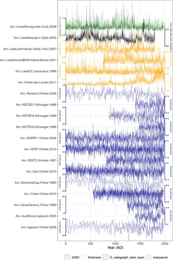
lections of sites. Here, we showcase how to use geoChronR
5.3 Age-uncertain calibration
to perform age-uncertain PCA (Sect. 3.3). When seeking to
analyze a large collection of datasets, the first, and often most
A natural extension of ensemble correlation is ensemble re- time-intensive, step is to track down, format, and standardize
gression, for which a common use case is calibrating a pa- the data. Fortunately, the emergence of community-curated
leoenvironmental proxy “in time” by regressing it against an standardized data collections (e.g., PAGES2K Consortium,
instrumental series using a period of overlapping measure- 2013; Emile-Geay et al., 2017; Kaufman et al., 2020b; Ko-
ments (Grosjean et al., 2009). We illustrate this by reproduc- necky et al., 2020) can greatly simplify this challenge. In this
ing the results of Boldt et al. (2015), who calibrated a spec- example, we examine the Arctic 2k database (McKay and
tral reflectance measure of chlorophyll abundance, relative Kaufman, 2014) and use geoChronR and the LiPD utilities to
absorption band depth (RABD), to instrumental temperature filter the data for temperature-sensitive data from the Atlantic
in northern Alaska. For each iteration in the analysis, a ran- Arctic with age ensembles relevant to the past 2000 years.
dom age ensemble member is chosen and used to bin the Once filtered, the data can be visualized using
RABD data onto a 3-year interval. The instrumental temper- plotTimeseriesStack, which is an option to quickly
ature data, here taken from the nearest grid cell of the NASA plot all of the time series, on their best-estimate age models,
Goddard Institute for Space Studies (GISS) Surface Tem- aligned on a common horizontal timescale (Fig. 7). Although
perature Analysis (GISTEMP) reanalysis product (Hansen all of the datasets are relevant to Arctic temperatures over
et al., 2010), are also binned onto the same timescale, ensur- the past 2000 years, they span different time intervals, with
ing temporal alignment between the two series. geoChronR variable temporal resolution. It is also clear that there is a lot
then fits an ordinary least squares model and then uses that of variability represented within the data, but it is difficult
model to “hindcast” temperature values from 3-year binned to visually extract shared patterns of variability. Ensemble
RABD data back in time. This approach propagates the age PCA identifies the modes of variability that explain the most
uncertainties both through the regression (model fitting) and variance within a dataset, while accounting for the impact of
prediction process. age uncertainty.
The function plotRegressEns produces multiple plots As in correlation and regression, aligning the data onto a
that visualize the key results of age-uncertain regression and common timescale is required for ensemble PCA. All but two
additionally creates an overview “dashboard” that showcases of these datasets are annually resolved, and the other two
the key results (Fig. 6). The first row of Fig. 6 illustrates have 5-year resolution, so it is reasonable to average these
the impact of age uncertainty on the regression modeling. data into 5-year bins. Furthermore, since many of the records
In this example, the distributions of the modeled parameters do not include data before 1400 CE, we only analyze the pe-
(the slope and intercept of the regression equation) show pro- riod from 1400 to 2000 CE. The data are now prepared for
nounced modes near 150 ◦ C−1 and −130 ◦ C, respectively, the ensemble PCA calculation, following a few choices in
but with pronounced tails that include models with much methodology and parameters. Because the data analyzed here
lower slopes. This is also apparent in the scatterplot in the have variable units, and we are not interested in the magni-
central panel of the top row, which illustrates the distribu- tude of the variance (only the relative variability between the
tion of modeled relationships. Although the tendency for ro- datasets), we choose to use a correlation, rather than covari-
bust relationships is clear, models with slopes near zero also ance, matrix. Next, we choose the number of components to
occur, suggesting that in this use case, age uncertainty can estimate. After the analysis, a scree plot is used to determine
effectively destroy the relationship with instrumental data. the number of significant components. We want to estimate
The impact of this variability in modeled parameters, as well several more components than we anticipate will be mean-
as the effects of age uncertainty on the timing of the recon- ingful. For this use case, we estimate eight components.
struction are shown in the bottom panel of Fig. 6. The results We now conduct the ensemble PCA, including null hy-
shown here are consistent with those presented by Boldt et al. pothesis testing, for 100 ensemble members. For a final anal-
https://doi.org/10.5194/gchron-3-149-2021 Geochronology, 3, 149–169, 2021You can also read