GPTuneBand: Multi-task and Multi-fidelity Autotuning for Large-scale High Performance Computing Applications
←
→
Page content transcription
If your browser does not render page correctly, please read the page content below
GPTuneBand: Multi-task and Multi-fidelity Autotuning for Large-scale High
                   Performance Computing Applications

                Xinran Zhu† , Yang Liu‡ , Pieter Ghysels‡ , David Bindel† , Xiaoye S. Li‡

Abstract                                                        In contrast, Bayesian optimization methods [21, 49, 17]
This work proposes a novel multi-task and multi-fidelity        typically model the tuning objective as a Gaussian pro-
autotuning framework, GPTuneBand, for tuning large-scale        cess (GP) [46], adaptively sample the objective to update
expensive high performance computing (HPC) applications.        the GP, and use the posterior GP as a surrogate model to
GPTuneBand combines a multi-task Bayesian optimization          search for new promising samples. When tuning expen-
algorithm with a multi-armed bandit strategy, well-suited       sive and noisy objectives, e.g., performance of large-scale
for tuning expensive HPC applications such as numerical         HPC applications, both methods face significant chal-
libraries, scientific simulation codes and machine learning     lenges due to the high cost of reliable samples. Strategies
(ML) models, particularly with a very limited tuning budget.    to address these challenges include:
Our numerical results show that compared to other state-             Multi-task tuning. In many tuning scenarios,
of-the-art autotuners, which only allows single-task or         there are correlated tuning tasks, and one can use such
single-fidelity tuning, GPTuneBand obtains significantly        correlation to improve performance on each task. Multi-
better performance for numerical libraries and simulation       task tuning has been used for continuous sets of tasks
codes, and competitive validation accuracy for training ML      [39, 38] and discrete tasks [31, 54, 44, 13, 35]. In the
models. When tuning the Hypre library with 12 parameters,       discrete case, one can use a multi-output GP model, such
GPTuneBand wins over its single-fidelity predecessor GPTune     as the linear coregionalization model (LCM) [3, 22] or the
on 62.5% tasks, with a maximum speedup of 1.2x, and wins        intrinsic model of coregionalization (IMC) [3, 18, 9], to
over a single-task, multi-fidelity tuner BOHB on 72.5% tasks.   model performance across correlated tasks [54, 44, 13, 35].
When tuning the MFEM library on large numbers of CPU            Some works further extended acquisition functions in
cores, GPTuneBand obtains a 1.7x speedup when compared          BO to multi-task settings [31, 54, 44, 13].
with the default code parameters.                                    Multi-fidelity tuning. Many applications can ex-
                                                                ecute at multiple fidelity levels, where the highest-fidelity
1    Introduction                                               runs correspond to the true, but most expensive objec-
                                                                tive function, and lower-fidelity ones are less accurate
Autotuning aims at automatically finding code param-
                                                                but computationally inexpensive. A multi-fidelity au-
eters that optimize the runtime, memory, communica-
                                                                totuner can run many low-fidelity evaluations (applica-
tion cost, or accuracy for complex, black-box functions.
                                                                tion runs) with smaller cost, quickly identify promis-
Specifically, this technique can be applied to hyperparam-
                                                                ing samples (parameter configurations), and then al-
eter tuning of ML models such as neural networks and
                                                                locate more resources for high-fidelity evaluations (ap-
support vector machines [7, 50, 8, 54, 29, 36, 30, 16, 57],
                                                                plication runs) with those samples (parameter config-
as well as tuning of performance-critical parameters for
                                                                urations). Some works focused on extending BO algo-
large-scale numerical libraries and first-principle simu-
                                                                rithms to multi-fidelity settings and adapted various
lation software packages [37, 35, 47]. Model-free opti-
                                                                acquisition functions in BO to multi-fidelity settings
mization and Bayesian optimization (BO) are two main
                                                                [19, 32, 23, 24, 45, 30, 57, 55]. Another line of work
families of black-box tuning methods. Model-free op-
                                                                is to use multi-armed bandit strategy for multi-fidelity
timization methods include global approaches such as
                                                                sampling to better balance low-fidelity evaluations and
simulated annealing [28], genetic algorithms [52] and par-
                                                                high-fidelity evaluations [33, 56].
ticle swarm optimization [26], and local approaches such
                                                                     To further improve tuner performance for large-scale
as Nelder–Mead simplex [41] and Orthogonal Search [11].
                                                                HPC applications, we propose GPTuneBand, a publicly
                                                                available autotuner allowing both multi-task and multi-
     † Cornell University, Ithaca, NY 14850, USA (xz584,        fidelity tuning. GPTuneBand is specially designed for
bindel@cornell.edu).
     ‡ Scalable Solvers Group, Lawrence Berkeley National       large-scale HPC applications, where application runs are
Laboratory, Berkeley, CA 94720, USA (liuyangzhuan, pghy-        expensive and limited to a relatively small number, but it
sels, xsli@lbl.gov).

                                                                                                    Copyright © 2022 by SIAM
                                                                            Unauthorized reproduction of this article is prohibited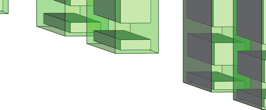
is also well suited for tuning any applications that needs optimization algorithms. OpenTuner does not support
multi-task tuning and allows multi-fidelity evaluations. multi-task or multi-fidelity tuning. Hyperband (HB) [33]
     Our main contributions are summarized below:            is a model-free multi-fidelity tuner based on the bandit
                                                             strategy and random sampling. It balances the number
   • GPTuneBand is an autotuning framework that of objective evaluations and the fidelity by using the ban-
      allows both multi-task and multi-fidelity tuning. dit strategy, and it will be described in detail in Section
      The key idea is to build LCM models across both 3.2. HpBandSter (BOHB) [16] is a BO variant of HB. It
      tasks and fidelity levels to guide sampling and differs from HB in that it builds Tree Parzen Estimator
      then use a multi-armed bandit strategy to select (TPE) [7] models to guide sampling. These tuners do
      potentially strong candidates from lower-fidelity not support multi-task tuning. Similarly, HB-ABLR [56]
      samples. Compared to neural network-based multi- is a multi-task and multi-fidelity tuning algorithm that
      task and multi-fidelity autotuners [56], our LCM- combines HB with adaptive Bayesian linear regression
      based lightweight autotuner requires much smaller (ABLR) [42]. However, it relies on neural networks, and
      numbers of samples to build informative models.        thus requires large number of evaluations, to build task
   • GPTuneBand applies to HPC codes on a variety correlation. GPTune [35] is a multi-task autotuning soft-
      of shared-memory or distributed-memory, CPU or ware package targeted at exascale applications, which
      CPU-based machine. In addition, GPTuneBand relies on LCM surrogate models to efficiently learn task
      itself is also distributed-memory parallel for the correlations. GPTune does not support multi-fidelity
      efficient modeling process.                            tuning, and it will be desribed in detail in Section 3.1. In
                                                             addition, a multi-task search space refinement algorithm
   • GPTuneBand is an extension of the publicly avail- [43] is also developed.
      able multi-task, single-fidelity autotuning frame-
      work GPTune [35], and therefore it is also publicly Algorithm 1 Bayesian optimization-based MLA
      available and inherits all salient features of GPTune, 1: Sampling: Evaluate y(x, ti ) at n = ntot /2 initial
      such as a historical database, crowd tuning, user-          random samples for each task ti ∈ T .
      provided performance models, and reverse communi- 2: while n < ntot do
      cation interface (RCI) to improve tuning efficiency. 3:         Modeling: Update hyperparameters of the
                                                                  LCM of {y(x, ti )}i≤m using all available data.
   • Our empirical study shows that GPTuneBand out-
                                                               4:     Search: Search for an optimizer x∗i for the EI
      performs several other state-of-the-art autotuners
                                                                  of task ti ∈ T . Let X ∗ = [x∗1 , x∗2 , . . . , x∗m ].
      on a wide range of large-scale scientific applications
                                                               5:     Evaluate y(x, ti ) for ti ∈ T at the new tuning
      as well as ML models.
                                                                  parameter configurations X ∗ .
     The paper is organized as follows. Section 2 discusses    6:     n ← n + 1.
related state-of-the-art work as our reference algorithms.     7: end  while
Section 3 introduces the notations of the general tuning       8: Return  the optimal tuning parameter configurations
problem, the multi-task tuning problem in the BO                  and  objective  function values for each task.
framework, and the multi-fidelity tuning problem in
the multi-armed bandit framework. Section 4 describes 3 Background
the GPTuneBand algorithm with an illustrative example. The goal of tuning is to find the parameter configurations
Section 5 shows the empirical study of GPTuneBand on that optimize an application’s performance such as
tuning various HPC and machine learning applications runtime, accuracy, or memory use. The tuning objective
and compare with the other state-of-the-art autotuners. is a function f : X → R over a d-dimensional tuning
                                                            parameter space X ⊂ Rd (discrete and categorical
2 Related work                                              parameters are mapped to R if needed). We model
In Section 1, we discussed related work in the general observations of the objective, which may be noisy, by
                                                                                                    2
autotuning literature, and related work specifically in the y(x) = f (x) +  where  ∼ N (0, σnoise     ). In the
multi-task tuning literature and multi-fidelity tuning lit- following, we describe the multi-task tuning algorithm
erature. Here, we highlight some specific stat-of-the-art of GPTune [35], and the multi-fidelity tuning algorithm
autotuners as the reference algorithms. OpenTuner [5] is of Hyperband [33], both of which are closely related to
one of the state-of-the-art model-free autotuners, which our GPTuneBand algorithm.
combines most of the model-free optimization algorithms
mentioned in Section 1 and then solves a multi-armed 3.1 Multi-task tuning in the BO framework
bandit problem [25] to allocate workloads to different In a multi-task setting, one has several tuning tasks

                                                                                                 Copyright © 2022 by SIAM
                                                                         Unauthorized reproduction of this article is prohibited
for an application, for example tuning the runtime of
a linear algebra solver on several different matrix sizes.                 µ∗ = Σ(X ∗ , X)Σ(X, X)−1 Y,
We parameterize tasks by t ∈ T ⊂ Rα , where T is an                       σ ∗2 = diag(Σ(X ∗ , X ∗ ) − Σ(X ∗ , X)Σ(X, X)−1 Σ(X, X ∗ )),
α-dimensional task space. The objective can then be                       which can be used to construct the EI acquisition
written as f (x, t) with one task argument t. We denote                   function. The EI is then optimized to select the next
by T = {t1 , t2 , . . . , tm } ⊂ T a set of m tuning tasks.               point X ∗ for each task. We refer to the GPTune paper
      The Efficient Global Optimization (EGO) [21] is                     [35] for more details on the search phase.
a classical BO algorithm that builds a Gaussian pro-                           One iteration finishes when a new sample X ∗ is
cess (GP) [46] as a surrogate model and then optimizes                    evaluated and it repeats until the sample budget ntot is
the Expected Improvement (EI) [40] acquisition func-                      exhausted. Algorithm 1 summarizes the MLA iterations.
tion to determine the next sample. The multi-task BO
algorithm used in GPTune, called the Multi-task Learn-
                                                                          Algorithm 2 Hyperband using SuccessiveHalving (SH)
ing Autotuning (MLA) algorithm, extends EGO to the
                                                                          as a subroutine
multi-task setting. MLA consists of three main phases:
                                                                          Inputs: η, fidelity bounds bmin and bmax
sampling, modeling and search [35].                                                            j          k
                                                                                                    b
      Sampling. MLA evaluates a set of n initial sam-                      1: compute smax = logη bmax .
                                                                                                      min
ples for each task. We let Xi ∈ Rd×n and Yi =                              2:   for s ∈ {smax , smax −1, . . . , 0} do
[yi,1 , . . . , yi,n ] ∈ Rn denote initial samples and evaluated                                       smax + 1 s
objective values for task ti , and X = [X1 , X2 , . . . , Xm ] ∈           3:      compute N (s) =                     η .
                                                                                                          s+1
Rd×nm and Y = [Y1 ; Y2 ; . . . ; Ym ] ∈ Rmn denote initial                 4:      compute B(s) = bmax η −s .
samples and evaluated objective values for all m tasks.                    5:      generate N (s) random samples at fidelity B(s)
      Modeling. MLA models the joint distribution                               and run SH on them.
across tasks by LCM [3, 22] which generalizes GPs to the                   6:   end for
multi-task setting. Specifically, LCM models objective
f (x, ti ) for each task ti ∈ T by linear combinations of
Q ≤ m latent random functions:
                                                                          3.2 Multi-fidelity tuning in the multi-armed
                                   Q
                                   X                                      bandit framework
                    f (x, ti ) =         ai,q uq (x),
                                                                          In a multi-fidelity setting, the application can be run with
                                   q=1
                                                                          different fidelity parameters, such as the discretization
where ai,q are hyperparameters to learn and uq (x) are                    level in a partial differential equation (PDE) solver, or
latent functions. Each latent function is an independent                  the number of iterations in an iterative algorithm. Lower
zero-mean GP with e.g., a squared exponential (SE)                        fidelity runs are less accurate, but are also less expensive.
kernel                                                                    We parameterize fidelities by b ∈ [bmin , bmax ], where
                               d
                                               !
                0     2
                              X
                                         0 2 q                            bmin , bmax are given minimum and maximum fidelity
        kq (x, x ) = σq exp −    (xi − xi ) /li ,
                                                                          levels. Here we assume the function evaluation time
                                       i=1
                                                                          is linear with the fidelity b. In this way, the objective
where σq2 is the variance and liq are length scales.                      function can be augmented as f (x, b) with one more
Thus, the covariance matrix for all samples of all tasks,                 fidelity input argument b. The tuning goal is to find
Σ(X, X) ∈ Rmn×mn , has entries                                            tuning parameters x to optimize the objective at the
                     Q
                     X                                                    highest fidelity, i.e., f (x, bmax ). Evaluations at a low
  Σ(xi,j , xi ,j ) =
             0  0      (ai,q ai0 ,q + bi,q δi,i0 )kq (xi,j , xi0 ,j 0 )
                      q=1
                                                                          fidelity f (x, b) where b < bmax serve as approximations
                                                                          of f (x, bmax ).
                      + di δi,i0 δj,j 0 ,                                      Hyperband (HB) [33] (Algorithm 2) is a recent
where δi,j is the Kronecker delta function, and bi,q                      model-free multi-fidelity tuning algorithm. Based on
and di are regularization parameters. The LCM model                       bandit strategy, it collects sets of random samples at
hyperparameters can then be estimated by maximizing                       different fidelity levels and then calls successive halv-
the log-likelihood using gradient-based optimization                      ing (SH) [20] (Algorithm 3) to promote promising sam-
methods such as L-BFGS [34].                                              ples to higher fidelity evaluations. Given a fidelity
      Search. The LCM predicts the joint distribution                     bound [bmin , bmax ] and a “halving” factor η, Hyperband’s
at new points [x∗1 , x∗2 , . . . , x∗m ] with posterior mean              multi-armed bandit strategy prescribes multiple brackets
µ∗ = [µ∗1 , µ∗2 , . . . , µ∗m ] and posterior variance σ ∗2 =             {0, 1, . . . , smax }, where 0 corresponds to the highest fi-
[σ1∗2 , σ2∗2 , . . . , σm
                        ∗2
                           ] as:                                          delity and smax = blogη bmax /bmin c. Thus, the associated
                                                                          fidelity levels are {bmax ' η smax bmin , . . . , ηbmin , bmin }, a

                                                                                                               Copyright © 2022 by SIAM
                                                                                       Unauthorized reproduction of this article is prohibited
geometrically decreasing sequence. Here bracket s re-       can execute multiple passes to collect more samples and
quires N (s) initial samples at fidelity B(s). Note that    build more informative LCMs. Using correlations across
bmin , bmax and η are designed for approximately equal      fidelities and tasks, GPTuneBand needs significantly
evaluation costs across brackets. After a bracket s col-    fewer total samples.
lects all initial samples, it evaluates all existing samples     Since LCM is used across both brackets and tasks,
in the bracket, keeps the best η ones, and evaluates them  we use “task” to refer to a user-specified tuning task, and
at a fidelity η times larger. This process repeats until   “LCM-task” to refer to a sub-task used to construct LCMs.
the highest fidelity bmax is reached in bracket s. Finally, Specifically, an “LCM-task” is a bracket associated with
Hyperband selects the best sample at the highest fidelity   a given fidelity level and a given tuning task. See Section
among all brackets.                                        4.1 for more details and examples.
     By using the multi-armed bandit strategy, Hyper-            Algorithm 4 summarizes the GPTuneBand algo-
band achieves good balance between the exploration via      rithm. The inputs are: a fidelity function B(·) mapping
low fidelity sampling and the exploitation via high fi-     a bracket variable s to a fidelity level B(s), a constant
delity sampling. Instead of generating random samples       smax determining the number of brackets, a constant
for SH, HpBandSter (BOHB) [16] generates samples for       “halving” factor η determining the number of samples
SH using BO methods via TPE [7] models. However,            of each bracket and the selection rate later in the SH
neither HB nor BOHB supports a multi-task tuning set-       run [20], and task parameters {ti }m      i=1 indicating tuning
ting. Moreover, even for single-task tuning, they do not    tasks. We explain Algorithm 4 in three stages:
exploit correlations among different fidelity levels during      Initialization stage. In this stage, we determine
sample collection.                                          the number of samples N (s) and the fidelity B(s) for each
                                                            bracket and each task. Given the constant smax , there
Algorithm 3 SuccessiveHalving                              will  be smax + 1 brackets indexed by bracket variables
Inputs: B(·), s, η, a set C containing N (s) configuration  s =  0, 1, . . . , smax . For bracket s, the number of samples
samples.                                                    N  (s) is geometrically-spaced:
 1:   for i ∈ {s, s − 1, . . . , 1} do                                     N (s) = b(smax + 1)/(s + 1)cη s .
 2:       Evaluate all configuration samples from C at
      B(i).                                                    The fidelity function B(·) maps a bracket variable s to
 3:       Select the top b|C|/ηc samples and form a new        a fidelity B(s), satisfying bmax = B(0) > B(1) · · · >
      sample set C.                                            B(smax ) = bmin . In this way, different from Hyperband
 4:   end for                                                  (Algorithm 2), we provide a more flexible way of bandit
 5:   Evaluate the current configuration sample set C at       sampling, but it reduces to the Hyperband setup by
      B(0).                                                    setting B(s) = bmax η −s and smax = blogη (bmax /bmin )c.
 6:   Return C containing selected samples at the highest      In the remaining part of this paper, for clarity we use
      fidelity.                                                the same setup as Hyperband and we refer to one input
                                                               tuple [bmin , bmax , η] as one specific bandit structure.
                                                                    Sampling stage. The next stage is to sample for
4     The GPTuneBand algorithm                                 all brackets of all tasks. The main for-loop in Algorithm
In this section, we introduce the proposed multi-task and      4 details the sampling approach. Specifically, it builds
multi-fidelity tuning algorithm GPTuneBand. Similar            LCMs across both brackets and tasks to guide the
to HpBandSter (BOHB), GPTuneBand has three stages.             sampling. We use the notation LCM(p, n) to represent
First, the bandit strategy prescribes the total number         one LCM with p LCM-tasks and n target samples for
of brackets, where bracket s requires N (s) samples at         each LCM-task. In line 5 of Algorithm 4, “build or
starting fidelity B(s). Second, BO algorithms are used         update LCM” works the same way as the MLA algorithm
to generate the N (s) samples in each bracket. Third,          (Algorithm 1) iteratively build and update an LCM.
each bracket runs the SH [20] algorithm (Algorithm 3)               Selection stage. When a bracket of one task has
to find the best one(s) in each bracket.                       finished the sampling stage, i.e., a bracket s reaches the
     We highlight several key differences between Hp-          target number of samples N (s), it will be removed from
BandSter and GPTuneBand: (a) While HpBandSter                  the LCM and enter the selection stage. It then calls an
build TPE models within each bracket to guide sam-             SH [20] run to identify the best one(s) at the highest
pling, GPTuneBand uses LCMs across fidelities in dif-          fidelity. At the end of the for-loop, after each bracket
ferent brackets to facilitate sampling. (b) GPTuneBand         identifies the best ones, GPTuneBand then reports the
extends well to the multi-task setting by using LCMs           best among them.
across both fidelity brackets and tasks. (c) GPTuneBand

                                                                                                   Copyright © 2022 by SIAM
                                                                           Unauthorized reproduction of this article is prohibited
s=0                    s=1                     s=2                       s=3

                   b=27
                   n=4      b=27           b=9
                            n=4            n=6
                                                       b=9         b=3
                                                       n=6         n=9
                 LCM(8,4)                                                     b=3
                                                                              n=9
                                                                                            b=1
                                                                                            n=27
                                      LCM(6,6)                                                        b=1
                                                                                                      n=27
                                                        LCM(4,9)
                                                                          LCM(2,27)
                                           b=27                    b=9
                                           n=2                     n=3                         b=3
                                                                                b=9
                   arm s user-task t SH                b=27
                                                       n=2                      n=3            n=9
                                                                                                         b=3
                                                  SH               b=27                                  n=9
                                                                   n=1          b=27           b=9
                                                              SH                n=1            n=3
                          samples n                                      SH                    b=27
                                                                                                         b=9
                                                                                                         n=3
                                                                                               n=1
                                                                                       SH                b=27
                                                                                                 SH      n=1

Figure 1: Illustrution of the proposed GPTuneBand algorithm with bmin = 1, bmax = 27, η = 3 and m = 2 tasks.
Number of samples and corresponding fidelity are denoted by n and b respectively.

4.1 Illustrative example of GPTuneBand                        Algorithm 4 GPTuneBand Algorithm (one pass)
In this section, we use a graphical example in Figure 1 to    Inputs: fidelity function B(·), smax , η, tasks: t1 , . . . ,tm
illustrate Algorithm 4. This example uses the bmin = 1,        1: Compute the starting number of samples N (s) for
bmax = 27, η = 3 bandit structure and m = 2 tasks. Each           each bracket     s:
solid vertical block represents one set of n samples at

                                                                                smax + 1 s
fidelity level b for one task. Each transparent horizontal     2: N (s) =                      η for s = 0, 1, . . . , smax .
                                                                                  s+1
block corresponds to one LCM (in gray, pink, orange            3: for s ∈ {0, . . . , smax } do
and blue). Each transparent vertical block represents          4:       build the current LCM-task set T = {Tij : i =
one SH run (in green).                                            1, . . . , m, j = s, . . . , smax }, where an LCM-task Tij
     From line 1 of Algorithm 4, for each of the two tasks,       means task ti with starting fidelity B(j).
it generates 4 brackets s = {0, . . . , 3}, with fidelities    5:
                                                                                                                 †
                                                                        build or update LCM(|T |, N (s)) , where |T | =
B(0) = 27, B(1) = 9, B(2) = 3, B(3) = 1, and number               m(smax − s + 1), until N (s) configuration samples
of samples N (0) = 4, N (1) = 6, N (2) = 9, N (3) = 27            for each task Tij ∈ T are obtained.
respectively. The main for-loop of Algorithm 4 contains        6:       run sucessive halving (SH) on each task Tij in
the sampling stage (LCM sampling) and the selection               bracket s, i.e. on T s = {Tij : i = 1, . . . , m, j = s}
stage (SH runs). We explain the LCM sampling and               7: end for
the SH runs separately even though they are done               8: Return Configuration with the optimal objective
concurrently in Algorithm 4.                                      value for each task ti .
     For the LCM sampling (Algorithm 4, lines 4 and 5),       † LCM(p, n) means an LCM model with p LCM-tasks, with
GPTuneBand first builds an LCM with m(smax + 1) = 8           n target samples for each LCM-task.
LCM-tasks and 4 samples each, using samples from all
brackets and tasks. Next, bracket s = 0 is removed from
LCM sampling and starts an SH run (Algorithm 4, line 6).      SH runs in total, 3 brackets s = 1, 2, 3 multiplied with 2
Without bracket s = 0, an LCM with msmax = 6 LCM-             tasks t = 1, 2 (bracket s = 0 requires no SH runs since
tasks and 6 samples each is then updated, which only          it collects samples at the highest fidelity bmax directly).
requires 2 more samples per LCM-task from 2 additional        For one task, each SH starts using N (s) samples at the
MLA search iterations (same as the MLA’s search phase         starting fidelity B(s), then boosts the fidelity for the top
in line 4 of Algorithm 1) as there exist 4 samples per        1/η = 1/3 configurations until the highest fidelity bmax
LCM-task from the previous LCM sampling. This LCM             is reached.
sampling process continues until all the brackets and              Algorithm 4 and Figure 1 only show one pass of
tasks have collected the target number of samples.            GPTuneBand, while in fact GPTuneBand can do multi-
     For the SH runs (Algorithm 4, line 6), it performs 6     pass tuning, with number of passes np > 1. In the first

                                                                                                      Copyright © 2022 by SIAM
                                                                              Unauthorized reproduction of this article is prohibited
pass, each LCM(p, n) generates n new samples per LCM- To compare multi-fidelity tuners GPTuneBand and
task from scratch. In the following passes, however, each BOHB, we use the same multi-armed bandit structure
LCM(p, n) generates n new samples per LCM-task on in both cases. To compare with single-fidelity tuners
top of all the historical data from previous passes, i.e., (GPTune, OpenTuner and TPE), which always run the
data generated by previous LCM sampling and SH runs. application at the highest fidelity, we use the same,
Therefore, more passes np could significantly improve normalized, total evaluation cost. Specifically, let the
the model quality of each LCM. highest fidelity evaluation have unit cost, an evaluation
at fidelity b would have normalized cost b/bmax . We
ensure the total sum of these normalized costs over all
samples at all fidelities for one task remains the same
across all autotuners.
Performance metrics. In multi-task settings, we
define three metrics to evaluate the tuning performance
of an autotuner. The absolute performance is the
final optimal objective values found by an autotuner,
while the relative performance is the ratio of the
optimal objective values found by an autotuner to the
optimal among all autotuners. Specifically, let {Ai }5i=1
be 5 autotuners. With tasks {tj }m j=1 , the absolute
performance of autotuner Ai is defined as
h i
RAi = oA Ai Ai
1 , o2 , . . . , om ,
i
and its relative performance is then
Figure 2: Example of multi-fidelity demo objective h
∗ Ai ∗ ∗
i
function for t ∈ [1, 1.5, 2, 2.5] with fidelity level b ∈ R̃Ai = oA Ai
1 /o1 , o2 /o2 , . . . , om /om ,
i
[1, 9, 27] and bmax = 27. where o∗j = min1≤i≤5 {oA j } is the best objective value of
i
task tj among all autotuners. Therefore, the closer each
entry of R̃Ai is to 1, the better the relative performance
5 Experiments autotuner Ai shows. For tuning with a relatively large
We run multi-task and multi-fidelity (MTMF) tuning number of tasks, we evaluate tuning performance by
to evaluate the tuning performance of GPTuneBand on comparing the distribution of R̃ over tasks {tj }m j=1 and
one synthetic function and four real numerical applica- use R̄ = (mean(R̃) + median(R̃))/2 as a metric to
tions: hypre [15], fast kernel ridge regression (KRR), evaluate the relative performance, the closer to 1 the
NIMROD [51], MFEM [4], and one machine learning model: better. In addition, for tuning with a small number
graph convolutional network (GCN). Experiments are of tasks, it is more straightforward to evaluate the
run on the Cori machine at NERSC1 : a Cray XC40 sys- tuning history, which is an array of historical best
tem with 2388 Haswell nodes, each of which consists of objective values found by an autotuner during objective
two 16-core Intel Xeon E5-2698v3 processors. Codes are evaluations on one task. We plot and compare the tuning
available online [1], and more experiment details can be history (on the highest fidelity) versus thus-far the total
found in the supplement2 . normalized evaluation cost (using all fidelities).
We compare with other state-of-the-art tuners:
GPTune [35], HpBandSter (BOHB) [16], TPE [7] and 5.1 Synthetic function
OpenTuner (OT) [5]. GPTune supports multi-task and We first run MTMF tuning on a 1D demo function. The
single-fidelity tuning; BOHB supports single-task and true objective is
multi-fidelity tuning; TPE is the single-fidelity version t+1 X 3
y(x, t) = 1 + e−(x+1) cos(2πx) sin 2πx(t + 2)i ,
of BOHB, i.e., a single-task BO algorithm based on
TPE models; OpenTuner supports single-task and single- i=1
fidelity tuning. where x ∈ [0, 1] and t > 0. This function is highly non-
convex, representing a very hard problem for black-box
1 http://www.nersc.gov/users/computational-systems/ optimization. The tuning goal is to minimize y(x, t) for
cori/ multiple tasks t. To enable multi-fidelity evaluations, we
2 https://drive.google.com/file/d/ add noise to the true objective, with a constant e = 0.1
1naLrGS73gBaDOQ83wpg7FzBHnb0JNCXJ/view?usp=sharing
Copyright © 2022 by SIAM
Unauthorized reproduction of this article is prohibited0.9 0.8
GPTuneBand, R = 1.010 2.5 0.9 0.7 GPTuneBand, R = 1.027
Optimal objective value Optimal objective value
0.6 BOHB GPTune 0.6
Optimal hypre time
0.95 GPTune 0.3 0.1 0.1 GPTuneBand, 9 wins GPTuneBand, 7 wins 0.3 0.2
GPTuneBand, 6 wins 0 2.0 0
0.1
0.85 0.9 BOHB, R = 1.082 1.5 0.9 BOHB, R = 1.343
0.6 0.5 0.6
0.3 0.3 0.2 0.3 0.10.1 0.10.1 0.10.10.10.1 0.10.1
0.75 BOHB 0 1.0 0
GPTuneBand, 9 wins 0.9 0.9
0.65 0.6 0.6 GPTune, R = 1.043 0.5 0.6 0.4 GPTune, R = 1.241
0.3 0.3 2.5 0.3
0.1 OpenTuner TPE 0.1 0.20.10.1 0.1
0 0
Optimal hypre time
GPTuneBand, 10 wins GPTuneBand, 8 wins
0.95 0.9 2.0 0.9
0.6 OpenTuner, R = 1.079 0.6 OpenTuner, R = 1.445
0.4 0.3
0.85 0.3 0.1 0.2 1.5 0.3 0.1 0.10.1 0.10.10.1 0.3 0.1
0 0
0.75 0.9 TPE, R = 1.112 1.0 0.9 TPE, R = 1.169
OpenTuner TPE 0.6 0.6 0.6
GPTuneBand, 9 wins GPTuneBand, 10 wins 0.3 0.3 0.3 0.3 0.20.10.1 0.20.1
0.65 1 2 3 4 5 6 7 8 9 10 0.1 0.5
1 2 3 4 5 6 7 8 9 10 0 1 1.05 1.1 1.15 1.2 1 2 3 4 5 6 7 8 9 10 1 2 3 4 5 6 7 8 9 10 0 1 1.2 1.4 1.6 1.8
Task ID Task ID Relative performance Task ID Task ID Relative performance
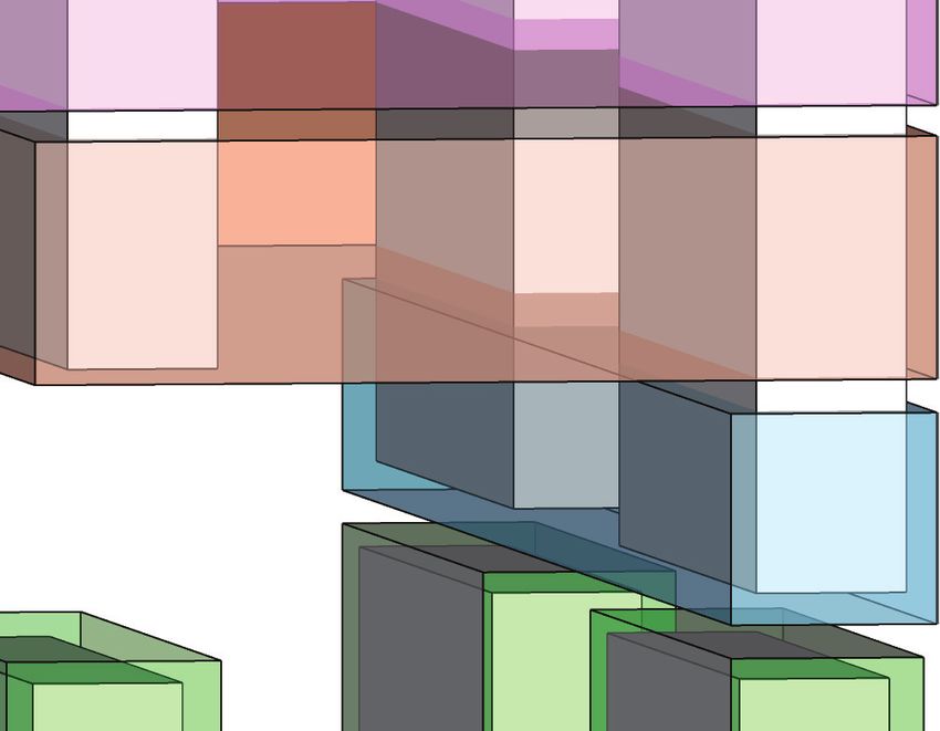
Ai
Figure 3: Detailed tuning results: 1) pair-wise comparison of absolute performance metric R and 2) histogram
plot of relative performance metric R̃Ai , where i = 1, ..., 5 correspond to five autotuners. Left: 10 demo tasks
corresponding to ID 1 of Table 1. Right: 10 hypre tasks corresponding to ID 3 of Table 2.
Bandit structure
ID Task range GPTuneBand BOHB GPTune OpenTuner TPE
[bmin ,bmax ,η]
1 [1, 1.45] [1, 8, 2] 1.010 1.082 1.043 1.079 1.112
2 [1, 1.45] [1, 16, 2] 1.018 1.064 1.039 1.054 1.094
3 [1, 1.45] [1, 9, 3] 1.022 1.088 1.023 1.092 1.114
4 [1, 1.45] [1, 27, 3] 1.017 1.017 1.050 1.060 1.051
5 [1, 1.45] [1, 16, 4] 1.016 1.025 1.030 1.086 1.084
6 [1, 5.5] [1, 27, 3] 1.013 1.090 1.107 1.131 1.090
Table 1: MTMF tuning of 10 demo tasks with different task ranges and different multi-armed bandit structures.
The relative performance metric R̄ of each autotuner is shown, the closer to 1 the better.
controlling the maximum noise level: structures, which work the best here.
ỹ(x, t, b) = y(x, t) (1 + e cos(ax)(1 − b/bmax )) .
5.2 HPC application: Hypre
Hence, ỹ(x, t, bmax ) = y(x, t) is an exact evaluation, The package hypre [15] contains several families of par-
while ỹ(x, t, bmin ) approximates y(x, t) with the least allel algebraic multigrid preconditioners and solvers for
accuracy. Figure 2 shows plots of demo function for large-scale sparse linear systems. Here we tune the
t ∈ [1, 1.5, 2, 2.5] with different fidelity levels b ∈ [1, 9, 27]. runtime of GMRES with the BoomerAMG precondi-
Specifically, b = bmax = 27 provides exact evaluation of tioner for solving the convection-diffusion equation on
the demo function y(x, t), while b = bmin = 1 and b = 9 structured 3D grids. Task parameters are defined by
provide approximate evaluations with different accuracy. the a, c coefficients in the convection-diffusion equation:
Using this demo, we study how different bandit −c∆u + a∇ · u = f. There are 12 tuning parameters of
structures affect the performance of GPTuneBand. We integer, real and categorical types, for example processor
select 10 tasks uniformly from a range of t and different topology parameters, total number of MPIs, the AMG
bandit structures. Each experiment uses np = 1 pass strength threshold, the type of the parallel coarsening
and is repeated for 5 runs. Table 1 compares the relative algorithm and the type of parallel interpolation operator.
performance, where GPTuneBand shows the best relative Details on tuning parameters can be found at [1].
performance for all experiments (rows). As for the The fidelity level is defined by the discretization
absolute performance, averaging over all 6 experiments, with k 3 grid points, where k ranges from kmin = 10 to
GPTuneBand wins over BOHB on 73% tasks, over kmax = 100. Given the O(k 3 ) computational complexity
GPTune on 67% tasks, over OT on 85% tasks, over of the algebraic multigrid algorithm, the fidelity mapping
TPE on 95% tasks. For more details, see Figure 3 (Left) 3
from b to k is a linear function interpolating [bmin , kmin ]
for the pair-wise comparison of absolute performance 3
and [bmax , kmax ]. Experiments are run on 2 NERSC
RAi and the histogram of relative performance R̃Ai for Cori nodes, with 5 repeated runs and np = 1 pass. Each
ID 1 in Table 1. We conclude that, for this example, highest-fidelity evaluation takes 5 seconds on average,
GPTuneBand performs the best and is not sensitive depending on the value of the tuning parameter.
to the choice of bandit structure. Therefore, in the Using hypre, we study how the multi-task setting
following, we mainly use the [1, 8, 2] and [1, 27, 3] affects the performance of GPTuneBand. We randomly
Copyright © 2022 by SIAM
Unauthorized reproduction of this article is prohibitedBandit structure
ID Task groups GPTuneBand BOHB GPTune OpenTuner TPE
[bmin , bmax , η]
1 10 [1, 8, 2] 1.20 1.25 1.02 1.49 1.23
2 10 [1, 27, 3] 1.11 1.16 1.01 1.35 1.10
3 5+5 [1, 27, 3] 1.03 1.34 1.24 1.46 1.17
4 3+2+3+2 [1, 27, 3] 1.03 1.27 1.13 1.53 1.19
5 3+3+4 [1, 27, 3] 1.09 1.29 1.08 1.39 1.14
6 3+3+4 [1, 8, 2] 1.10 1.19 1.10 1.34 1.13
Table 2: MTMF tuning of 10 hypre tasks with different task groups: m1 + m2 represents one m1 -task tuning and
one m2 -task tuning. Each task group performs an independent GPTune/GPTuneBand multi-task tuning. The
relative performance metric R̄ of each autotuner is shown, the closer to 1 the better.
select 10 tasks with a, c ∈ [0, 1] and break tasks into simultaneously without any grid search as in [12].
different groups for multi-task tuning. This task group Given the linear-complexity of HSS-enhanced KRR,
division only affects multi-task tuners GPTune and we define the fidelity by the percentage p of total training
GPTuneBand, which perform an independent multi-task data, where pmin = 0.5 to pmax = 1. Therefore, the
tuning per group. fidelity level is linear with evaluation cost. With the
A comparison of relative performance is summarized validation set fixed to 1K, a low-fidelity evaluation uses
in Table 2. From Table 2, GPTuneBand outperforms partial training data, while a highest-fidelity evaluation
almost all tuners but GPTune in 10-task tuning (ID uses all training data. Given a bandit structure
1&2). However, if the same 10 tasks are divided into [bmin , bmax , η], the fidelity mapping from b to p is a linear
smaller multi-task groups (ID 3,4,5,6) with each group function interpolating [bmin , pmin ] and [bmax , pmax ]. We
containing tasks of similar coefficients a, c, GPTuneBanduse the [bmin , bmax , η] = [1, 27, 3] bandit structure with
then performs the best or nearly best. As for the np = 3 passes. Each highest-fidelity evaluation requires
absolute performance, with smaller groups, on average about 5 seconds on 2 NERSC Cori nodes.
GPTuneBand wins over BOHB on 72.5% tasks, over A comparison of the tuning history is summarized
GPTune on 62.5% tasks, over OT on 85% tasks, and over in Figure 4. Tuning histories are averaged over 5 runs,
TPE on 65% tasks. For more details, see Figure 3 (Right) with the shaded area being the standard error. We
for the pair-wise comparison of absolute performance note that, on average, GPTuneBand outperforms its
RAi and the histogram plot of relative performance R̃Ai single-fidelity counterpart GPTune. For the first task
for ID 3 in Table 2. On hypre, BOHB, however, cannot on the left, all tuners, except TPE, find a good enough
even outperform its single-fidelity version TPE, whereas objective value fairly quickly and they also reach very
GPTuneBand shows effective multi-fidelity tuning. similar final results. TPE performs the worst on the
For the observation that smaller groups improve first task. For the second task, though all tuners reach
GPTuneBand to outperform GPTune, one intuitive similar final results, earlier tuning performance differs
reason is that, for the same set of tasks, GPTuneBand a lot. Noticeably, GPTuneBand outperforms all tuners,
builds more and larger size of LCMs than GPTune, which except only TPE; BOHB cannot even outperform its
is more difficult to fit due to more LCM hyperparameters,single-fidelity counterpart TPE and showed very large
especially for large task counts. performance variances. Generally, on the two tasks
among all tuners, GPTuneBand performs stably well
5.3 HPC-ML application: linear-complexity with small variances, and consistently outperforms its
kernel ridge regression (KRR) single-task counterpart GPTune.
We run MTMF tuning of the KRR validation accuracy
on datasets from the public repository [14]. We consider 5.4 ML application: graph convolutional net-
two tasks/datasets SUSY [6] and Occupancy [10], with work (GCN)
N = 10K and N = 8K training data respectively. We We run MTMF tuning on another ML application us-
use a linear-complexity (in N ) KRR algorithm using the ing GPUs. The tuning goal is the validation accuracy
distributed-memory numerical software STRUMPACK[53] of a graph convolutional network (GCN) [27] for semi-
with the HSS compression algorithm. The tuning setting supervised graph node classification. We tune four GCN
is similar to Algorithm 5 of [12] with two real-valued hyperparameters3 : number of hidden units, initial learn-
tuning parameters: the length scale h in the Gaussian
kernel and the regularization parameter λ in ridge re- 3 We use the GCN implementation in https://github.com/
gression. Here we use the 5 autotuners to tune h and λ tkipf/pygcn.
Copyright © 2022 by SIAM
Unauthorized reproduction of this article is prohibitedFigure 4: Tuning history of KRR on 2 tasks/datasets: SUSY (Left) and Occupancy (Right). Averaged over 5 runs.
Plots are the historically best function values at the highest fidelity versus thus-far the total normalized evaluation
cost using all fidelities.
ing rate, dropout rate for all layers, and weight decay (the of one function evaluation is proportional to t, we map
L2 regularization factor in the GCN loss). We set up two a fidelity level b to number of time steps t by linearly
graph datasets Cora [48] and Citeseer [48] as two tasks. interpolating between [bmin , tmin ] and [bmax , tmax ].
The fidelity is defined by the number of training epochs For fast and reliable evaluations of the tuning
K ranging from Kmin = 100 to Kmax = 500. Given objective, we use the so-called reverse communication
a bandit structure [bmin , bmax , η], the fidelity mapping interface (RCI, see Section 3.2.2 of [2]). However,
from b to K is a linear function interpolating [bmin , Kmin ] other autotuners (OpenTuner, BOHB or TPE) do not
and [bmax , Kmax ]. We use the [bmin , bmax , η] = [1, 27, 3] support RCI, and therefore we only apply GPTune
bandit structure with np = 4 passes. Each evaluation at and GPTuneBand to tune NIMROD. Tuning histories
highest fidelity requires several seconds using 1 NERSC are plotted in Figure 6 (left). GPTuneBand is able
Cori GPU (NVIDIA Tesla V100 GPU). to find better runtime faster than GPTune, and the best
A comparison of the tuning history is summarized runtime is about 7% faster than the default parameter
in Figure 5. Tuning histories are averaged over 10 runs, configuration (the first sample in Figure 6).
with the shaded area being the standard error. We note
that, on average, GPTuneBand not only finds the best 5.6 HPC Application: MFEM
final objective value, but also optimizes the performance We also run single-task and multi-fidelity tuning on an-
faster than other tuners. For this example, GPTuneBand other large-scale HPC application MFEM. MFEM [4] is a
shows efficient multi-task and multi-fidelity tuning. high-performance scalable finite element discretization
library, containing a collection of discretization algo-
5.5 HPC Application: NIMROD rithms, linear system solvers, and application drivers.
In addition, we run single-task, multi-fidelity tuning Here we focus on using first order Nédélec elements on
on a large-scale HPC application NIMROD for modeling tetrahedral mesh to discretize a unit cube for solving
reactor-scale tokamaks. NIMROD is a time-marching code highly indefinite Maxwell equations. Once the linear
for modeling extended magnetohydrodynamic equations, system is constructed, we solve it with the multi-frontal
whose most computationally expensive component is sparse solver STRUMPACK[53] with block low-rank (BLR)
solving multiple nonsymmetric sparse linear systems compression algorithms.
using SuperLU DIST at each time step. In this experiment, we consider single-task tuning of
In this experiment, we consider single-task tuning total MFEM runtime using 16 NERSC Cori nodes. There
of the marching time by fixing a geometry model and are three tuning parameters indicating the number of
discretization with 16 NERSC Cori nodes and a total OpenMP threads per MPI, cutoff size of BLR compressed
of 512 MPIs. We pick four integer tuning parameters fronts, and leaf sizes in BLR compression. The fidelity
affecting computation granularity of matrix assembly in level is defined by the mesh resolution on the geometry.
NIMROD and matrix factorization in SuperLU DIST. The Specifically, we use the [bmin , bmax , η] = [1, 8, 8] bandit
fidelity level is defined by the number of time steps t, structure, corresponding to linear systems of size N =
where tmin = 3 to tmax = 30. Given that the runtime 1872064 (high fidelity) and N = 238688 (low fidelity).
Copyright © 2022 by SIAM
Unauthorized reproduction of this article is prohibitedFigure 5: Tuning history of GCN on 2 tasks/datasets Cora (Left) and Citeseer (Right). Averaged over 10 runs.
Plots are the historically best function values at the highest fidelity versus thus-far the total normalized evaluation
cost using all fidelities.
Figure 6: (Left) Tuning history of NIMROD: single task, bandit structure [bmin , bmax , η] = [1, 8, 2]. Averaged
over 4 runs with the shaded area being the standard error. (Right) Tuning history of FMEM: single task, bandit
structure [bmin , bmax , η] = [1, 8, 8]. Averaged over 7 runs with the shaded area being the standard error.
Same as NIMROD, we only use the RCI-enabled GPTune multi-fidelity setting, inherits all features of GPTune,
and GPTuneBand to tune MFEM. Tuning results are and is also publicly available. Limitations, and there-
plotted in Figure 6 (right). GPTuneBand is able to fore future developing directions of GPTuneBand may
find better runtime faster than GPTune, and the best include: 1) a more rigorous investigation on task correla-
runtime is about 1.7x (1.7 times) faster than the default tions, 2) an improvement of GPTuneBand on multi-task
parameter configuration (the first sample in Figure 6). tuning for a large number of tasks, 3) a relaxation of
the multi-task modeling, to allow different number of
6 Conclusion samples for each task in the LCM modeling.
We developed GPTuneBand, a gernal tuning framework
that supports both multi-task and multi-fidelity (MTMF) Acknowledgement
tuning, well-suited for tuning large-scale HPC applica- This research was supported by the Exascale Computing
tions when the number of application runs is limited. Project (17-SC-20-SC), a collaborative effort of the U.S.
GPTuneBand outperforms other state-of-the-art auto- Department of Energy Office of Science and the National
tuners on the MTMF tuning of a wide range of numer- Nuclear Security Administration, and by the National
ical software packages and machine learning methods. Science Foundation under CCF-1934985 and the Simons
GPTuneBand is implemented within the framework of foundation. We used resources of the National Energy
GPTune, which is a recently developed, publicly avail- Research Scientific Computing Center (NERSC), a U.S.
able, multi-task autotuner. Therefore, GPTuneBand Department of Energy Office of Science User Facility
essentially extends the GPTune tuning framework to a operated under Contract No. DE-AC02-05CH11231.
Copyright © 2022 by SIAM
Unauthorized reproduction of this article is prohibitedReferences [12] Gustavo Chávez, Yang Liu, Pieter Ghysels, Xi-
[1] GPTune. https://github.com/gptune/GPTune. aoye Sherry Li, and Elizaveta Rebrova. Scalable and
memory-efficient kernel ridge regression. In 2020 IEEE
[2] GPTune user guide. https://gptune.lbl.gov/ International Parallel and Distributed Processing Sym-
documentation/gptune-user-guide. posium (IPDPS), pages 956–965, 2020.
[3] Mauricio A. Alvarez, Lorenzo Rosasco, and Neil D.
[13] Sihui Dai, Jialin Song, and Yisong Yue. Multi-task
Lawrence. Kernels for vector-valued functions: A review.
Bayesian optimization via Gaussian process upper
Foundations and Trends in Machine Learning, 4(3):195–
confidence bound. In ICML 2020 Workshop on Real
266, 2012.
World Experiment Design and Active Learning, 2020.
[4] Robert Anderson, Julian Andrej, Andrew Barker, Jamie
Bramwell, Jean-Sylvain Camier, Jakub Cerveny, Veselin [14] Dheeru Dua and Casey Graff. UCI Machine Learning
Dobrev, Yohann Dudouit, Aaron Fisher, Tzanio Kolev, Repository. Irvine, CA: University of California, School
Will Pazner, Mark Stowell, Vladimir Tomov, Ido of Information and Computer Science, 2017.
Akkerman, Johann Dahm, David Medina, and Stefano
Zampini. MFEM: A modular finite element methods [15] Robert D. Falgout and Ulrike Meier Yang. hypre:
library. Computers and Mathematics with Applications, A library of high performance preconditioners. In
81:42–74, 2021. International Conference on Computational Science
(ICCS), pages 632–641. Springer Berlin Heidelberg,
[5] Jason Ansel, Shoaib Kamil, Kalyan Veeramachaneni, 2002.
Jonathan Ragan-Kelley, Jeffrey Bosboom, Una-May
O’Reilly, and Saman Amarasinghe. Opentuner: An [16] Stefan Falkner, Aaron Klein, and Frank Hutter. BOHB:
extensible framework for program autotuning. In Pro- Robust and efficient hyperparameter optimization at
ceedings of the 23rd International Conference on Parallel scale. In Proceedings of the 35th International Confer-
Architecture and Compilation Techniques (PACT), pages ence on Machine Learning, volume 80, pages 1437–1446.
303–315, 2014. PMLR, 2018.
[6] Pierre Baldi, Peter Sadowski, and Daniel Whiteson. [17] Peter I Frazier. Bayesian optimization. In Recent Ad-
Searching for exotic particles in high-energy physics vances in Optimization and Modeling of Contemporary
with deep learning. Nature Communications, 5:4308, Problems, pages 255–278. INFORMS, 2018.
2014.
[7] James Bergstra, Rémi Bardenet, Yoshua Bengio, and [18] Pierre Goovaerts et al. Geostatistics for natural resources
Balázs Kégl. Algorithms for hyper-parameter optimiza- evaluation. Oxford University Press on Demand, 1997.
tion. In Advances in Neural Information Processing
Systems, volume 24, page 2546–2554. Curran Associates, [19] Deng Huang, Theodore T Allen, William I Notz,
Inc., 2011. and R Allen Miller. Sequential kriging optimization
using multiple-fidelity evaluations. Structural and
[8] James Bergstra, Daniel Yamins, and David Cox. Making Multidisciplinary Optimization, 32(5):369–382, 2006.
a science of model search: Hyperparameter optimization
in hundreds of dimensions for vision architectures. In [20] Kevin Jamieson and Ameet Talwalkar. Non-stochastic
Proceedings of the 30th International Conference on best arm identification and hyperparameter optimiza-
Machine Learning, volume 28, pages 115–123. PMLR, tion. In Proceedings of the 19th International Conference
2013. on Artificial Intelligence and Statistics, volume 51, pages
240–248. PMLR, 2016.
[9] Edwin V Bonilla, Kian Chai, and Christopher Williams.
Multi-task Gaussian process prediction. In Advances [21] Donald R Jones, Matthias Schonlau, and William J
in Neural Information Processing Systems, volume 20, Welch. Efficient global optimization of expensive black-
pages 153–160. Curran Associates, Inc., 2008. box functions. Journal of Global Optimization, 13(4):455–
[10] Luis M Candanedo and Véronique Feldheim. Accurate 492, 1998.
occupancy detection of an office room from light,
temperature, humidity and CO2 measurements using [22] Andre G Journel and Charles J Huijbregts. Mining
statistical learning models. Energy and Buildings, 112:28– geostatistics. Academic Press, 1976.
39, 2016.
[23] Kirthevasan Kandasamy, Gautam Dasarathy, Junier
[11] Timothy M Chan, Kasper Green Larsen, and Mihai Oliva, Jeff Schneider, and Barnabás Póczos. Gaussian
Pătraşcu. Orthogonal range searching on the RAM, process bandit optimisation with multi-fidelity evalua-
revisited. In Proceedings of the twenty-seventh annual tions. In Advances in Neural Information Processing
symposium on Computational geometry (SOCG), pages Systems, volume 29, page 1000–1008. Curran Associates,
1–10, 2011. Inc., 2016.
Copyright © 2022 by SIAM
Unauthorized reproduction of this article is prohibited[24] Kirthevasan Kandasamy, Gautam Dasarathy, Jeff [36] Hector Mendoza, Aaron Klein, Matthias Feurer, Jost To-
Schneider, and Barnabás Póczos. Multi-fidelity Bayesian bias Springenberg, and Frank Hutter. Towards
optimisation with continuous approximations. In Inter- automatically-tuned neural networks. In Workshop on
national Conference on Machine Learning, volume 70, Automatic Machine Learning, pages 58–65. PMLR, 2016.
pages 1799–1808. PMLR, 2017.
[37] Harshitha Menon, Abhinav Bhatele, and Todd Gamblin.
[25] Michael N Katehakis and Arthur F Veinott Jr. The Auto-tuning parameter choices in HPC applications us-
multi-armed bandit problem: decomposition and compu- ing Bayesian optimization. In 2020 IEEE International
tation. Mathematics of Operations Research, 12(2):262– Parallel and Distributed Processing Symposium (IPDPS),
268, 1987. pages 831–840. IEEE, 2020.
[26] James Kennedy and Russell Eberhart. Particle swarm [38] Jan Hendrik Metzen. Minimum regret search for single-
optimization. In Proceedings of the International and multi-task optimization. In Proceedings of The
Conference on Neural Networks (ICNN), volume 4, pages 33rd International Conference on Machine Learning,
1942–1948. IEEE, 1995. volume 48, pages 192–200. PMLR, 2016.
[27] Thomas N. Kipf and Max Welling. Semi-supervised [39] Jan Hendrik Metzen, Alexander Fabisch, and Jonas
classification with graph convolutional networks. In Hansen. Bayesian optimization for contextual policy
Proceedings of the 5th International Conference on search. In Proceedings of the Second Machine Learning
Learning Representations (ICLR), 2017. in Planning and Control of Robot Motion Workshop.
[28] Scott Kirkpatrick, C Daniel Gelatt, and Mario P IROS Hamburg, 2015.
Vecchi. Optimization by simulated annealing. Science, [40] Jonas Močkus. On Bayesian methods for seeking
220(4598):671–680, 1983. the extremum. In Proceedings of the IFIP Technical
[29] Aaron Klein, Simon Bartels, Stefan Falkner, Philipp Conference, pages 400–404. Springer, 1975.
Hennig, and Frank Hutter. Towards efficient Bayesian
[41] John A Nelder and Roger Mead. A simplex method for
optimization for big data. In NIPS 2015 Bayesian
function minimization. The Computer Journal, 7(4):308–
Optimization Workshop, 2015.
313, 1965.
[30] Aaron Klein, Stefan Falkner, Simon Bartels, Philipp
[42] Valerio Perrone, Rodolphe Jenatton, Matthias Seeger,
Hennig, Frank Hutter, et al. Fast Bayesian hyperparam-
and Cédric Archambeau. Scalable hyperparameter trans-
eter optimization on large datasets. Electronic Journal
fer learning. In Proceedings of the 32nd International
of Statistics, 11(2):4945–4968, 2017.
Conference on Neural Information Processing Systems,
[31] Andreas Krause and Cheng Ong. Contextual Gaussian pages 6846–6856, 2018.
process bandit optimization. In Advances in Neural
Information Processing Systems, volume 24, pages 2447– [43] Valerio Perrone, Huibin Shen, Matthias W Seeger,
2455. Curran Associates, Inc., 2011. Cedric Archambeau, and Rodolphe Jenatton. Learning
search spaces for bayesian optimization: Another view
[32] Rémi Lam, Douglas L Allaire, and Karen E Willcox. of hyperparameter transfer learning. Advances in Neural
Multifidelity optimization using statistical surrogate Information Processing Systems, 32:12771–12781, 2019.
modeling for non-hierarchical information sources. In
56th AIAA/ASCE/AHS/ASC Structures, Structural [44] Matthias Poloczek, Jialei Wang, and Peter I Frazier.
Dynamics, and Materials Conference, page 0143, 2015. Warm starting Bayesian optimization. In 2016 Winter
Simulation Conference (WSC), pages 770–781. IEEE,
[33] Lisha Li, Kevin Jamieson, Giulia DeSalvo, Afshin Ros- 2016.
tamizadeh, and Ameet Talwalkar. Hyperband: A novel
bandit-based approach to hyperparameter optimization. [45] Matthias Poloczek, Jialei Wang, and Peter I Frazier.
The Journal of Machine Learning Research, 18(1):6765– Multi-information source optimization. In Advances
6816, 2017. in Neural Information Processing Systems, volume 30,
pages 4291–4301. Curran Associates, Inc., 2017.
[34] Dong C Liu and Jorge Nocedal. On the limited memory
BFGS method for large scale optimization. Mathematical [46] Rasmussen, Carl Edward and Williams, Christopher K.
Programming, 45(1):503–528, 1989. I. Gaussian Processes for Machine Learning. The MIT
Press, 2006.
[35] Yang Liu, Wissam M Sid-Lakhdar, Osni Marques,
Xinran Zhu, Chang Meng, James W Demmel, and [47] Rohan Basu Roy, Tirthak Patel, Vijay Gadepally, and
Xiaoye S Li. GPTune: Multitask learning for autotuning Devesh Tiwari. Bliss: Auto-Tuning Complex Appli-
exascale applications. In Proceedings of the 26th ACM cations Using a Pool of Diverse Lightweight Learning
SIGPLAN Symposium on Principles and Practice of Models, page 1280–1295. Association for Computing
Parallel Programming, pages 234–246, 2021. Machinery, New York, NY, USA, 2021.
Copyright © 2022 by SIAM
Unauthorized reproduction of this article is prohibited[48] Prithviraj Sen, Galileo Namata, Mustafa Bilgic, Lise
Getoor, Brian Galligher, and Tina Eliassi-Rad. Col-
lective classification in network data. AI Magazine,
29(3):93, 2008.
[49] Bobak Shahriari, Kevin Swersky, Ziyu Wang, Ryan P
Adams, and Nando De Freitas. Taking the human out
of the loop: A review of Bayesian optimization. In
Proceedings of the IEEE, volume 104, pages 148–175.
IEEE, 2016.
[50] Jasper Snoek, Hugo Larochelle, and Ryan P Adams.
Practical bayesian optimization of machine learning al-
gorithms. In Advances in Neural Information Processing
Systems, volume 25, page 2951–2959. Curran Associates,
Inc., 2012.
[51] C.R. Sovinec, A.H. Glasser, T.A. Gianakon, D.C. Barnes,
R.A. Nebel, S.E. Kruger, S.J. Plimpton, A. Tarditi, M.S.
Chu, and the NIMROD Team. Nonlinear magnetohy-
drodynamics with high-order finite elements. Journal
of Computational Physics, 195:355, 2004.
[52] Mandavilli Srinivas and Lalit M Patnaik. Genetic
algorithms: A survey. Computer, 27(6):17–26, 1994.
[53] STRUMPACK – STRUctured Matrix PACKage, version
5.1.1, 2021.
[54] Kevin Swersky, Jasper Snoek, and Ryan Prescott Adams.
Multi-task Bayesian optimization. In Advances in Neural
Information Processing Systems, volume 26, pages 2004–
2012. Curran Associates, Inc., 2013.
[55] Shion Takeno, Hitoshi Fukuoka, Yuhki Tsukada,
Toshiyuki Koyama, Motoki Shiga, Ichiro Takeuchi, and
Masayuki Karasuyama. Multi-fidelity Bayesian opti-
mization with max-value entropy search and its par-
allelization. In Proceedings of the 37th International
Conference on Machine Learning, volume 119, pages
9334–9345. PMLR, 2020.
[56] Lazar Valkov, Rodolphe Jenatton, Fela Winkelmolen,
and Cédric Archambeau. A simple transfer-learning
extension of hyperband. In NIPS Workshop on Meta-
Learning, 2018.
[57] Jian Wu, Saul Toscano-Palmerin, Peter I Frazier,
and Andrew Gordon Wilson. Practical multi-fidelity
Bayesian optimization for hyperparameter tuning. In
Proceedings of the 35th Uncertainty in Artificial Intelli-
gence Conference, volume 115, pages 788–798. PMLR,
2020.
Copyright © 2022 by SIAM
Unauthorized reproduction of this article is prohibitedYou can also read