Herbaceous perennial plants with short generation time have stronger responses to climate anomalies than those with longer generation time - Nature
←
→
Page content transcription
If your browser does not render page correctly, please read the page content below
ARTICLE
                  https://doi.org/10.1038/s41467-021-21977-9                 OPEN

                  Herbaceous perennial plants with short generation
                  time have stronger responses to climate anomalies
                  than those with longer generation time
                  Aldo Compagnoni 1,2 ✉, Sam Levin1,2, Dylan Z. Childs 3, Stan Harpole 1,2,4, Maria Paniw5, Gesa Römer6,7,
                  Jean H. Burns 8, Judy Che-Castaldo9, Nadja Rüger2,10,11, Georges Kunstler 12, Joanne M. Bennett 1,2,13,
                  C. Ruth Archer14,15, Owen R. Jones 6,7, Roberto Salguero-Gómez16,18 & Tiffany M. Knight 1,2,17,18
1234567890():,;

                  There is an urgent need to synthesize the state of our knowledge on plant responses to
                  climate. The availability of open-access data provide opportunities to examine quantitative
                  generalizations regarding which biomes and species are most responsive to climate drivers.
                  Here, we synthesize time series of structured population models from 162 populations of 62
                  plants, mostly herbaceous species from temperate biomes, to link plant population growth
                  rates (λ) to precipitation and temperature drivers. We expect: (1) more pronounced demo-
                  graphic responses to precipitation than temperature, especially in arid biomes; and (2) a
                  higher climate sensitivity in short-lived rather than long-lived species. We find that pre-
                  cipitation anomalies have a nearly three-fold larger effect on λ than temperature. Species with
                  shorter generation time have much stronger absolute responses to climate anomalies. We
                  conclude that key species-level traits can predict plant population responses to climate, and
                  discuss the relevance of this generalization for conservation planning.

                  1 Martin Luther University Halle-Wittenberg, Halle (Saale), Germany. 2 German Centre for Integrative Biodiversity Research (iDiv) Halle-Jena-Leipzig,

                  Leipzig, Germany. 3 Department of Animal and Plant Sciences, University of Sheffield, Sheffield, UK. 4 Department of Physiological Diversity, Helmholtz-
                  Centre for Environmental Research—UFZ, Leipzig, Germany. 5 Department of Evolutionary Biology and Environmental Studies, University of Zurich,
                  Winterthurerstrasse 190, Zurich CH-8057, Switzerland. 6 Interdisciplinary Center on Population Dynamics, University of Southern Denmark, Odense
                  M, Denmark. 7 Department of Biology, University of Southern Denmark, Odense M, Denmark. 8 Department of Biology, Case Western Reserve University,
                  Cleveland, OH, USA. 9 Alexander Center for Applied Population Biology, Conservation & Science Department, Lincoln Park Zoo, Chicago, IL, USA.
                  10 Smithsonian Tropical Research Institute, Apartado, Balboa, Ancón, Panama. 11 Department of Economics, University of Leipzig, Leipzig, Germany. 12 Univ.

                  Grenoble Alpes, INRAE, UR LESSEM, Grenoble, France. 13 Centre for Applied Water Science, Institute for Applied Ecology, The University of Canberra,
                  Canberra, Australian Capital Territory, Canberra, Australia. 14 Centre for Ecology and Conservation, College of Life and Environmental Sciences, University of
                  Exeter, Penryn, UK. 15 Institute of Evolutionary Ecology and Conservation Genomics, University of Ulm, Ulm, Germany. 16 Department of Zoology, University
                  of Oxford, Oxford, UK. 17 Department of Community Ecology, Helmholtz Centre for Environmental Research–UFZ, Halle (Saale), Germany. 18These authors
                  jointly supervised this work: Roberto Salguero-Gómez, Tiffany M. Knight. ✉email: aldo.compagnoni@idiv.de

                  NATURE COMMUNICATIONS | (2021)12:1824 | https://doi.org/10.1038/s41467-021-21977-9 | www.nature.com/naturecommunications                                    1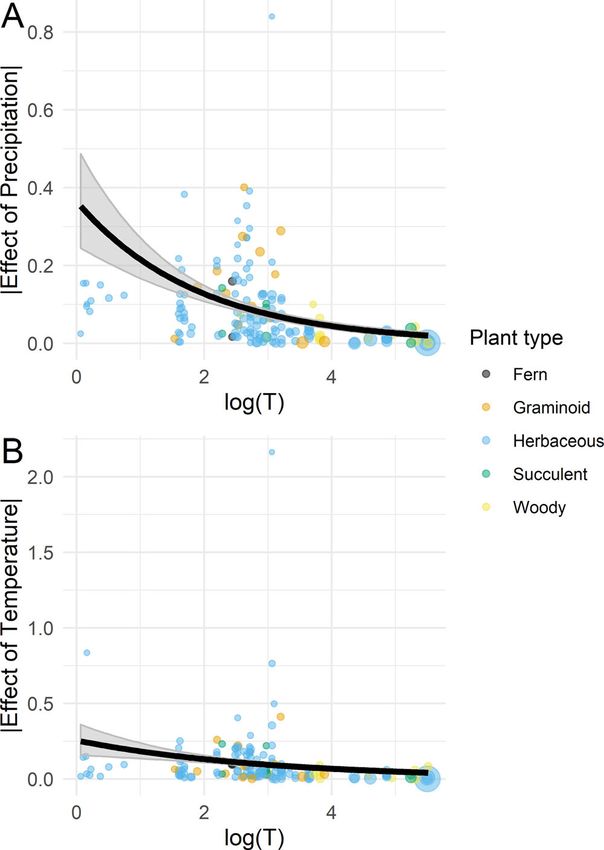
ARTICLE NATURE COMMUNICATIONS | https://doi.org/10.1038/s41467-021-21977-9
C
limate change is altering the mean as well as the variance generation time to respond more weakly to temperature and
in temperature and precipitation worldwide1. These precipitation anomalies. We show that the effect of precipitation
changes in climate are widely recognized as a prime global is three times larger than that of temperature (H1). Moreover,
threat to biodiversity2 because temperature and precipitation larger generation times are associated with weaker responses to
ultimately drive the demographic processes that determine the climate (H4). Both of these findings will inform ecological fore-
size and long-term viability of natural populations3. Hence, it is casts, and the result on generation time emphasizes the impor-
critical to evaluate which species are most responsive to climatic tance of this life-history trait to conservation assessments.
drivers, and in which biomes4. The urgency to understand the
response of species to climate is particularly high for species that Results
cannot buffer against the effects of climate change by migrating, Our model selection provided little evidence for nonlinear
such as sessile species. Among sessile species, numerous plants responses to climate, and little evidence of interactions between
have short-distance dispersal, and cannot, therefore, shift their climatic and non-climatic factors. A nonlinear model was selected
ranges fast enough to keep up with the current pace of climate in eight of the 38 populations for which we tested nonlinear
change5,6. relationships (Supplementary Figs. 3–5). We, therefore, con-
Assuming plant productivity is a proxy of population perfor- sidered a linear relationship for the remaining 154 populations;
mance, we expect that precipitation, or its interaction with tem- we present these linear relationships in the online repository that
perature, predicts plant population growth better than also contains the data and code related to this study21. Only two
temperature alone. Most plant physiological processes, such as populations showed a substantial effect of the interaction between
seed germination, tissue growth, floral induction, and seed set, are climate anomalies and covariates: our only population of Astra-
affected by water availability7. Accordingly, precipitation is a key galus cremnophylax var. cremnophylax, and one of Dicerandra
driver of vegetation productivity worldwide8. Temperature can frutescens (Supplementary Data 1). These interactions increased
also influence these processes, but typically by modulating water the estimates of the climatic effect by 40 times (from 0.001 to
availability9, as plant growth occurs across a wide range of tem- 0.052) and decreased it by 16% (from −0.189 to −0.158),
peratures (namely between 5 and 40 °C7,10). The effect of tem- respectively.
poral fluctuations on the growth rate of a population should be
proportional to precipitation or temperature anomalies, where The overall effect of climate on plant population growth rate.
anomalies are deviations from mean values. As predicted (H1), the overall effect of precipitation anomalies on
Precipitation and temperature anomalies are expected to have a log(λ) was strong (β = 0.031, 95% CI: 0.007–0.054) relative to
more pronounced effects in arid and cold biomes than in wet and that of temperature (η = −0.013, 95% CI: −0.036 to 0.009) and
temperate ones. While species should be adapted to their their interaction (θ = −0.008, 95% CI: −0.029 to 0.011), which
respective environment, extreme environments impose hard were centered around zero. On average, a year with precipitation
physiological limitations. In arid environments, plants experience one standard deviation above the mean changed λ by +3.3%.
water limitation more frequently11. Similarly, in cold biomes
plants should more frequently experience temperatures that are
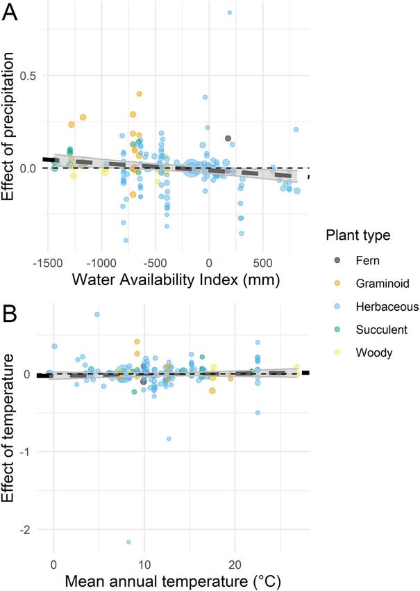
too low to allow tissue growth10,12. Accordingly, as water avail- The effect of biome on the response of plants to climate. The
ability decreases, precipitation becomes the main factor limiting meta-regressions testing the response of plant populations to
plant physiological processes13,14. On the other hand, in cold precipitation (H2) and temperature (H3) anomalies were both
biomes temperature anomalies can be disproportionately nonsignificant (Fig. 1). When testing the correlation between
important. For example, the temperature has a positive effect on WAI and the response of plant populations to precipitation
tree growth that increases in explanatory power with altitude15,16. anomalies, only 90.5% of our bootstrap samples had slopes below
Similarly, in the tundra temperature anomalies can dramatically zero (βmeta = −3.83 × 10⁻⁵, 95% CI: −9.47 × 10⁻⁵, 1.99 × 10⁻⁵).
change the length of the growing season17. However, because Similarly, we did not find evidence that the mean annual tem-
plant functional composition is filtered by biome18, it is impor- perature (H3) of the site predicted the response of plant popu-
tant to consider whether differences in the responses of plants lations to temperature anomalies (Fig. 1b; βmeta = −1.42 × 10⁻³,
across biomes might be due to the different composition of plant 95% CI: −6.62 × 10⁻³, 1.00 × 10⁻²).
functional types (graminoids, herbs, ferns, woody species, and
succulents) that occur in those biomes. The effect of generation time on the response of plants to
The life-history theory also provides expectations for how climate. We found strong support for the effect of generation
natural plant populations may respond to climate drivers. The time (H4) on the absolute response of plant populations to cli-
key life-history trait defining plant life-history strategy is gen- mate. As expected, the response of species to climate correlated
eration time, which describes how fast individuals in a population negatively with generation time (Fig. 2). In these meta-regres-
are substituted and is correlated with life expectancy19. The sions, 100% of simulated βmeta values referring to the effect of
population growth of long-lived species should respond weakly to precipitation (βmeta = −0.54, 95% CI: −0.63 to −0.44]), and
climatic anomalies compared to short-lived species. We expect temperature (βmeta = −0.40, 95% CI: −0.50 to −0.30]) were
this because the long-run population growth rate of long-lived below zero.
species responds less strongly to increases in the temporal var-
iation of survival, growth, and reproduction20. Here, we capitalize The effect of plant types on estimates of climate effects. The
on the recent availability of large volumes of demographic data to effect of precipitation (P < 0.01), but not temperature (P = 0.97),
quantitatively test how to plant population growth rate, λ, changed based on organism type according to the ANOVA tests.
responds to temperature and precipitation anomalies. We expect Tukey’s honestly significant difference test showed a significant
(H1) λ to be more strongly associated with precipitation than difference in the effect of precipitation between herbaceous and
temperature anomalies, because we expect water availability to graminoid species (Supplementary Tables 2 and 3, Supplementary
having stronger physiological effects than temperature; (H2) λ of Fig. 6). We, therefore, re-run separate tests of H2, and H4
plants in water-limited biomes to be more responsive to pre- excluding the precipitation effect sizes of graminoid species. We
cipitation anomalies; (H3) λ of plants in cold biomes to be more excluded graminoid species only because herbaceous species
responsive to temperature anomalies; (H4) species with greater comprised 127 of our 162 populations so that excluding them
2 NATURE COMMUNICATIONS | (2021)12:1824 | https://doi.org/10.1038/s41467-021-21977-9 | www.nature.com/naturecommunicationsNATURE COMMUNICATIONS | https://doi.org/10.1038/s41467-021-21977-9 ARTICLE
Fig. 1 The effect of precipitation and temperature anomalies as a function Fig. 2 The absolute effect of precipitation and temperature anomalies as
of site mean aridity and temperature. Effect of precipitation (A) and a function of logged generation time (T). We show the effect sizes of
temperature (B) anomalies on the logged asymptotic population growth precipitation and temperature anomalies as a function of log(T) (panels A
rate (λ) as a function of water availability index (A) and mean annual and B, respectively). The uncertainty of these effect sizes is shown by the
temperature (B). The y-axis represents the effect sizes of yearly anomalies size of circles, which are inversely proportional to the standard error (SE) of
in precipitation and temperature. The uncertainty of these effect sizes is effect sizes (1/SE). The thick black lines show the mean prediction of the
shown by the size of circles, which are inversely proportional to the meta-regressions. The shaded areas represent the 95% confidence interval
standard error (SE) of effect sizes (1/SE). The thick black lines show the of 1000 bootstrapped gamma regressions. The color of individual data
mean prediction of the meta-regressions; these lines are dashed because points shows five separate plant types.
these relationships are nonsignificant. The shaded areas represent the 95%
confidence interval of 1000 bootstrapped linear regressions. The color of
individual data points shows five separate plant types. more strongly to climate. These generalizations, especially the one
on generation time, are relevant to conservation planning and
would not provide meaningful inferences. In these additional tests evolutionary theory. However, because the available data is biased
discarding graminoid data, H2 was not supported, and H4 was towards herbaceous perennials of temperate regions, our results
upheld. In H2, the percentage of simulated βmeta values lower than might not be universal.
zero was 72%, well below the 90.4% of the full dataset (Supple- The large, positive effect of precipitation on a log(λ) and the
mentary Methods, Supplementary Fig. 7). On the other hand, H4 negative, smaller effects of temperature and its interaction
was upheld, with 100% of βmeta below zero (Supplementary with precipitation are consistent with the importance of water
Methods, Supplementary Fig. 8). availability on plant population performance25 and productivity8.
The importance of precipitation as a driver of plant popula-
tion growth implies highly uncertain ecological forecasts. Climate
Discussion change projections involving precipitation are much more
While quantifying population responses to climate drivers has a uncertain than those involving temperature23. Moreover, pre-
long history in plant ecology22, there is an urgent need to syn- diction uncertainty in climate projections is not expected to
thesize our knowledge due to on-going climate change4,23. The improve much in the coming decades27. As a result, accounting
availability of open-access data24, a solid understanding of phy- for this uncertainty will be a fundamental step when crafting
siological ecology25, and a mature evolutionary theory of life ecological forecasts of plant populations (e.g., model
histories26 provide opportunities to produce quantitative gen- uncertainty28).
eralizations regarding plant population responses to climate. In To our knowledge, our results are the first to show that gen-
our global synthesis, we found that (H1) precipitation has a eration time is linked to population responses to climatic drivers
stronger effect on population growth rates than temperature and across a large number of species. To our knowledge, the only
that (H4) plant species with shorter generation time respond other study to test for this hypothesis found a similar pattern for
NATURE COMMUNICATIONS | (2021)12:1824 | https://doi.org/10.1038/s41467-021-21977-9 | www.nature.com/naturecommunications 3ARTICLE NATURE COMMUNICATIONS | https://doi.org/10.1038/s41467-021-21977-9
three amphibian species29. We formulated our hypothesis linking characteristic of graminoids, or, as we originally expected (H2), of
generation time to population responses to climate because in a arid biomes. In future studies, disentangling the role of biomes
sample of long-lived plants and animals, Morris et al20. found and taxonomic bias on plant climate sensitivity will require study
that the long-run population growth rate responds little to designs that stratify plant types across biomes.
increases in the variation of survival and reproduction. Our The predictive ability of our results, which use as predictors of
results are complementary to this seminal study, in that the low annual climatic anomalies calculated from gridded climatic data,
sensitivity to climate drivers we found in long-lived species could be improved in the future by mechanistic models that use
should minimize the variation in yearly population growth rates. increasingly more available microclimatic information44. Gridded
Such minimized variation in yearly population growth rates is climatic data are adequate to estimating climatic means registered
linked to higher long-run population growth rates30–32. Hence, by weather stations over long time periods, such as years45.
we demonstrated that it is possible to use plant traits to predict However, the temperature experienced by plant tissues can
which species will be most sensitive to climate change4. Inter- sometimes be substantially different from the air temperature
estingly, generation time is a fundamental quantity in identifying registered by weather stations46,47. We note, however, that this
extinction probability33,34. It is, therefore, a good news that this fact does not invalidate the use of gridded climatic data, because
trait can also predict the climatic sensitivity of herbaceous plants. annual anomalies observed at the microclimatic and weather
The fact that responses to climate do not change based on station level should be similar. For example, a previous study
biome suggests that plant populations are demographically shows a tight linear relationship between air temperature and the
adapted to cope with climate variation regardless of the average microclimate at the leaf surface in alpine vegetation47. Never-
climate. In extreme environments, the stronger effect of climate theless, microclimatic data will be required to test mechanistic
on the variation of ecosystem processes such as productivity14,35 models of climatic effects, such as those linked to thresholds.
or biomass accumulation15,16 is not reflected in demographic Examples of these thresholds are growing degree days48
patterns. It is, therefore, plausible that adaptations such as (Mcmaster 1997) or frost damage49. Similarly, microclimatic
investment in survival36 or dormancy37 are sufficient to de- anomalies could help understand why different populations of the
couple physiological processes from demographic patterns. Such same species respond differently to comparable climatic
de-coupling is crucial because if climate drove larger variance in anomalies50.
population growth rates, this would decrease the chances of Our findings on the link between short generation times and
population persistence. However, because plants appear adapted climatic sensitivity do not automatically translate into climate
to local climatic variation, these results do not mean that all vulnerability. The observational nature of our data imposes to
biomes will be equally vulnerable to climatic change. Rather, interpret our findings in light of two caveats. First, our data did
vulnerability to climate change will likely depend on how changes not address several of the concurrent factors that contribute to
in climate compare to pre-existing climatic variability38. the effects of climate on populations. These include factors such
The geographic and taxonomic bias of our dataset might as density-dependence3, trophic interactions51, and anthro-
amplify the relevance of precipitation anomalies, and it therefore pogenic drivers52. Second, our results are more relevant to
may affect the generality of our findings. First, geographic bias changes in climatic variability than changes in climatic means.
potentially underemphasizes the role of temperature, because of When predicting the effects of large changes in climatic means,
our dataset under-samples extremely cold and hot biomes. For our nonlinear results (Supplementary Figs. 3–5) show that
example, in cold biomes such as montane or boreal forests, the extrapolation might not be warranted. Besides these two caveats,
influence of temperature on growth is larger as the mean annual the conservation literature links short generation times to lower,
temperature decreases15,16. On the other hand, the interaction rather than higher climate vulnerability as indicated by our
between precipitation and temperature may be larger in hot than results53,54. These studies reflect conservation assessments which
in colder biomes9. Therefore, we might expect a strong interac- posit that short generation time should be linked to lower
tion between precipitation and temperature anomalies where extinction probability33. Short-generation time should also
mean precipitation is low and mean temperature high. These increase the probability of evolutionary rescue55. However, the
conditions should occur, for example, in the subtropical desert or advantages provided by short generation time might be over-
tropical savannas, but only a handful of our studies occur in these ridden by the rapid rates of climate change expected. Thus,
biomes (Supplementary Fig. 1). Similarly, the taxonomic bias in weighing the positive and negative effects of generation time will
our data could also amplify the importance of precipitation leverage our findings to improve the quality of climate change
anomalies. For example, our dataset contained only two trees and vulnerability assessments.
five shrubs. However, woody species have surprisingly effective
adaptations to cope with water shortages39, and they could
therefore be susceptible only to extreme precipitation anomalies. Methods
Demographic data. To address our hypotheses, we used matrix population models
Nevertheless, we note that inferences dominated by herbaceous (MPMs) or integral projection models (IPMs) from the COMPADRE Plant Matrix
perennials have high significance globally. At least 40% of ter- Database (v. 5.0.156) and the PADRINO IPM Database57, which we amended with
restrial habitats are dominated by grasslands40, herbaceous spe- a systematic literature search. First, we selected density-independent models from
cies comprise most of the biodiversity in temperate forests41, and COMPADRE and PADRINO which described the transition of a population from
1 year to the next. Among these, we selected studies with at least six annual
they have a critical role in the carbon cycle42. transition matrices, to balance the needs of adequate yearly temporal replicates and
Our data on graminoids exemplify that the covariation between sufficient sample size for a quantitative synthesis. This yielded data from 48 species
taxonomies and biomes complicates the interpretation of global and 144 populations.
comparative studies. In our results, the response of graminoids to We then performed a systematic literature search for studies linking climate
drivers to structured population models in the form of either MPMs or IPMs. We
precipitation anomalies is larger than other plant types, and this performed this search on ISI Web of Science for studies published between 1997
response drives the positive correlation between WAI and the and 2017. We used a Boolean expression containing keywords related to plant
effect of precipitation (Fig. 1a). Moderately arid climates favor form, structured demographic models, and environmental drivers (Supplementary
grasses43, which might have an inherent advantage in exploiting Methods). We only considered studies linking macro-climatic drivers to natural
populations (e.g., transplant experiments and studies focused on local climatic
precipitation or at least precipitation pulses that increase the factors such as soil moisture, light due to treefall gaps, etc. were excluded). Finally,
moisture of shallow soil horizons11. As a result, we cannot we used the same criteria used to filter studies in COMPARE and PARDINO, by
establish whether sensitivity to precipitation anomalies is selecting studies with at least six, density-independent, annual projection models.
4 NATURE COMMUNICATIONS | (2021)12:1824 | https://doi.org/10.1038/s41467-021-21977-9 | www.nature.com/naturecommunicationsNATURE COMMUNICATIONS | https://doi.org/10.1038/s41467-021-21977-9 ARTICLE
This search brought two additional species, belonging to three additional these metrics, we downloaded data at 1 km2 resolution for mean annual potential
populations, which we entered in the COMPADRE database. evapotranspiration, mean annual precipitation, and mean annual temperature
One of the studies we excluded from the literature search because it contained referred to the 1970–2000 period. We obtained potential evapotranspiration data
density-dependent IPMs, also provided raw data with high temporal replication from the CGIAR-CSI consortium (http://www.cgiar-csi.org/). This dataset
(14–32 years of sampling) for 12 species from 15 populations58. Therefore, we re- calculates potential evapotranspiration using the Hargreaves method69. We
analyzed these freely available data to produce density-independent MPMs that obtained mean annual precipitation and mean annual temperature from
were directly comparable to the other studies in our dataset (Supplementary Worldclim70. Here, we used WorldClim rather than CHELSA climatic data because
Methods). the CGIAR-CSI potential evapotranspiration data were computed from the former.
The resulting dataset consisted of 46 studies, 62 species, 162 populations, and a We calculated the WAI values at each of our sites by subtracting mean annual
total of 3761 MPMs and 52 IPMs (Supplementary Data 1). The analyzed plant potential evapotranspiration from the mean annual precipitation. Such proxy is a
populations were tracked for a mean of 16 (median of 12) annual transitions. To coarse measure of plant water availability that ignores information such as soil
our knowledge, this is the largest open-access dataset of long-term structured characteristics and plant rooting depth. However, WAI is useful to compare water
population projection models. However, this dataset is taxonomically and availability among disparate environments, so that it is often employed in global
geographically biased. Specifically, among our 62 species, this dataset contains 54 analyses68,71. As our proxy of temperature limitation, we use mean annual
herbaceous perennials (11 of which graminoids), and eight woody species: five temperature. While growing degree days would be a more mechanistic measure of
shrubs, two trees, and one woody succulent (Opuntia imbricata). Moreover, almost temperature limitation48, this requires daily weather data. However, we could not
all of these studies were conducted in North America and Europe (Supplementary find a global, downscaled, daily gridded weather dataset to calculate this metric.
Fig. 1), in temperate biomes that are cold, dry, or both cold and dry
(Supplementary Fig. 1, inset). Our geographic and taxonomic bias reflects the rarity
The overall effect of climate on plant population growth rate. To test H1, we
of long-term plant demographic data in general. This dearth of long-term
estimated the overall effect sizes of responses to anomalies in temperature, pre-
demographic data is particularly evident in the tropics. The ForestGEO network59
cipitation, and their interaction with a linear mixed-effect model.
is an exception to this rule, but to date, no matrix population models or integral
projection models using these data have been published. logðλÞ ¼ α þ βP þ ηT þ θPxT þ ε ð1Þ
We used the MPMs and IPMs in this dataset to calculate the response variable
of our analyses: the yearly asymptotic population growth rate (λ). This measure is where log(λ) is the log of the asymptotic population growth rate of plant popu-
one of the most widely used summary statistics in population ecology60, as it lation P is precipitation, T is temperature. We included random population effects
integrates the response of multiple interacting vital rates. Specifically, λ reflects the on the intercept and the slopes to account for the nonindependence of measure-
population growth rate that a population would attain if its vital rates remained ments within populations. We then compared the mean absolute effect size of
constant through time61. This metric therefore distills the effect of underlying vital precipitation, temperature, and their interaction. This final model did not include a
rates on population dynamics, free of other confounding factors (e.g., transient quadratic term of temperature and precipitation because these additional terms led
dynamics arising from population structure62). We calculated λ of each MPM or to convergence issues. This likely occurred because single data sets did not include
IPM with standard methods61,63. Because our MPMs and IPMs described the enough years of data.
demography of a population transitioning from one year to the next, our λ values
were comparable in time units. Finally, we identified and categorized any non- Population-level effect of climate on plant population growth rates. To test our
climatic driver associated with these MPMs and IPMs. Data associated with 21 of remaining three hypotheses, we carried out meta-regressions where the response
our 62 species explicitly quantified a non-climatic driver (e.g., grazing, neighbor variable was the slope (henceforth “effect size”) of climatic anomalies on the
competition), for a total of 60 of our 162 populations. Of the datasets associated population growth rate for each of our populations. Before carrying out our meta-
with these species, 19 included discrete drivers, and only three included a regression, we first estimated the effect size of our two climatic anomalies on the
continuous driver. population growth rate of each population separately. We initially fit population-
level and meta-regression simultaneously, in a hierarchical Bayesian framework.
However, these Bayesian models shrunk the uncertainty of the noisiest
Climatic data. To test the effect of temporal climatic variation on demography, we population–level relationships, resulting in unrealistically strong meta-regressions.
gathered global climatic data. We downloaded 1 km2 gridded monthly values for We, therefore, chose to fit population models separately, resulting in more con-
maximum temperature, minimum temperature, and total precipitation between servative results.
1901 and 2016 from CHELSAcruts64, which combines the CRU TS 4.0165, and For each population, we fit multiple regressions with an autoregressive error
CHELSA66 datasets. Gridded climatic data are especially suited to estimate annual term, and we evaluated the potential for nonlinear effects in the datasets longer
climatic means45. These datasets include values from 1901 to 2016, which are than 14 years. We fit multiple regressions because temperature and precipitation
necessary to cover the temporal extent of all 162 plant populations considered in anomalies were negatively correlated, so that fitting separate models for
our analysis. For our temperature analyses, we calculated the mean monthly temperature and precipitation would yield biased results72. We fit an autoregressive
temperature as the mean of the minimum and maximum monthly temperatures. error term because density dependence and autocorrelated climate anomalies can
We used monthly values to calculate the time series of mean annual temperature produce autocorrelated plant population growth rates. The form of our baseline
and total annual precipitation at each site. We then used this dataset to calculate model was
our annual anomalies for each census year, defined as the 12 months preceding a
population census. Our annual anomalies are standardized z-scores. For example, if logðλÞy ¼ α þ βp Py þ βt Ty þ εy ð2Þ
X is a vector of 40 yearly precipitation or temperature values, E() calculates the
mean, and σ() calculates the standard deviation, we compute annual anomalies as εy ¼ ρεy1 þ ηy ð3Þ
A = [X − E(X)]/σ(X). Therefore, an anomaly of one refers to a year where pre-
cipitation or temperature was one standard deviation above the 40-year mean. In The model in Eq. 2 is a linear regression relating each log(λ) data point observed in
other words, anomalies represent how infrequent annual climatic conditions are at year y, to the corresponding precipitation (P) and temperature (T) anomalies
a site. Specifically, if we assume that A values are normally distributed, values observed in year y, via the intercept α, the effect sizes, β, and an error term, εy,
exceeding one and two should occur every 6 and 44 years, respectively. We used which depends on white noise, ηy, and on the correlation with the error term of the
40-year means because the minimum number of years suggested to calculate cli- previous year, ρ. When multiple spatial replicates per each population were
mate averages is 3067. available each year, we estimated the ρ autocorrelation value separately for each
Z-scores are commonly used in global studies on vegetation responses to replicate. This happened in the few cases when a study contained contiguous
climate8,68, and they reflect the null hypothesis that species are adapted to the populations, with no ecologically meaningful (e.g., habitat) differences.
climatic variation at their respective sites. Across our populations, the standard We compared the baseline model in Eqs. 2 and 3 to models including a
deviations of annual precipitation and temperature anomalies change by 300% and quadratic climatic effect and non-climatic covariates. We estimated quadratic
60%, respectively (Supplementary Fig. 2). Thus, a z-score of one refers to a climatic effects only for time series longer than 14 years. We choose this threshold
precipitation anomaly of 50 or 160 mm and to a temperature anomaly of 0.5 or 0.8 because when using a model selection approach to select a quadratic or linear
°C. Our null hypothesis posits that species are adapted to these conditions, regression model, the recommended minimum sample size is between 8 and 25
regardless of the absolute magnitude of the standard deviation in annual climatic data points73. We fit models including a quadratic effect of temperature,
anomalies. If this null hypothesis were true, each species would respond similarly to precipitation, or both (Supplementary Table 1).
z-scores. Z-scores are more easily interpreted when calculated on normally Finally, we also tested whether non-climatic covariates could bias the effects of
distributed variables. We found our temperature and precipitation z-scores were climate on log(λ) estimated in our analysis. Such bias, either upwards or
highly skewed (skewness above 1) only in, respectively, 2 (for temperature) and downwards, could result in the case non-climatic co-variates interacted with
three (for precipitation) of our 162 populations. We concluded that this degree of climate. For example, harvest can have multiplicative, rather than additive effects
skewness should not bias our z-scores substantially. on the climate responses of forest understory herbs74. We tested for an interaction
To test how the response of plant populations to climate changes based on between a covariate and climate anomaly in 17 of the 21 studies that included a
biome we used two proxies of water and temperature limitation. For each study non-climatic covariate. In the remaining three studies, discrete covariates
population, we computed a proxy for water limitation, water availability index corresponded with the single populations. Because Eqs. 2 and 3 is fit on separate
(WAI), and temperature limitation using mean annual temperature. To compute populations, it implicitly accounted for these covariates. For the 17 studies above,
NATURE COMMUNICATIONS | (2021)12:1824 | https://doi.org/10.1038/s41467-021-21977-9 | www.nature.com/naturecommunications 5ARTICLE NATURE COMMUNICATIONS | https://doi.org/10.1038/s41467-021-21977-9
we fit a linear effect of the non-climatic covariate and its interaction with one of the Reporting summary. Further information on research design is available in the Nature
two linear climatic anomalies. Thus, including the linear model in Eqs. 2 and 3, the Research Reporting Summary linked to this article.
nonlinear models, and the covariate interaction models, we tested up to six
alternative models for each one of our populations (Supplementary Table 1). We
selected the best model according to the Akaike Information Criterion corrected Data availability
for small sample sizes (AICc75). We carried out these and subsequent analyses in R Most of the demographic data used in this paper are open-access and available in the
version 3.6.176. COMPADRE Plant Matrix Database (v. 5.0.1; https://compadre-db.org/Data/
In the populations for which AICc selected one of the model alternatives to the Compadre). Additional data come from the PADRINO Database (beta version; https://
baseline in Eqs. 2 and 3, we calculated the effect size of climate by adding the effect github.com/levisc8/rpadrino). A list of the studies and species used here is available in
of the new terms to the linear climatic terms. For example, when a quadratic Supplementary Data 1. The CHELSAcruts dataset is available at 10.16904/envidat.159.
precipitation model was selected, we calculated the effect size of precipitation as The formatted dataset, and associated metadata, to reproduce the analyses of this study
β = βp + βp2. For models including an interaction between temperature and a non- are archived on Github at https://doi.org/10.5281/zenodo.4516446.
climatic covariate, we evaluated the effect of the interaction at the mean value of
the covariate. Therefore, we calculated the effect size as β = βt + βxE(Ci) for
continuous covariates. For categorical variables, we calculated the effect size as
Code availability
The code to reproduce the results of this study is stored on Github at https://doi.org/
βp + βx0.5: that is, we calculated the mean effect size between the two categories.
We quantified the standard error of the resulting effect sizes by adding the standard 10.5281/zenodo.4516446.
errors of the two terms.
Received: 2 July 2020; Accepted: 16 February 2021;
The effect of biome on the response of plants to climate. We used a simulation
procedure to run two meta-regressions to test for the correlation between the effect
size of climate drivers on λ, and our measures of water or temperature limitation.
These meta-regressions accounted for the uncertainty, measured as the standard
error, in the effect sizes of climate drivers. We represented the effect of biome using
a proxy of water (WAI) and temperature (mean annual temperature) limitation.
For each of our 162 populations, the response data of this analysis were the effect
References
1. IPCC. Climate Change 2013: The Physical Science Basis. Contribution of
sizes (βp or βt values) estimated by Eqs. 2 and 3 or their modifications in case a
Working Group I to the Fifth Assessment Report of the Intergovernmental Panel
quadratic or non-climatic covariate model were selected. In these meta-regressions,
the weight of each effect size was inversely proportional to its standard error. To on Climate Change. (Cambridge University Press, 2013).
test H2 and H3 on how water and temperature limitation should affect the response 2. Willis, K. J. & Bhagwat, S. A. Biodiversity and Climate Change. Science 326,
of populations to climate, we used linear meta-regressions. These two hypotheses 806–807 (2009).
tested both the sign and magnitude of the effect of climate. Therefore, we used the 3. Ehrlén, J. & Morris, W. F. Predicting changes in the distribution and abundance
effect sizes as a response variable which could take negative or positive values. As of species under environmental change. Ecol. Lett. 18, 303–314 (2015).
predictors, we used population-specific WAI (H2, only for effect sizes quantifying 4. Sutherland, W. J. et al. Identification of 100 fundamental ecological questions.
the effect of precipitation), and mean annual temperature (H3, only for effect sizes J. Ecol. 101, 58–67 (2013).
quantifying the effect of temperature). The null hypothesis of these meta-regres- 5. Jump, A. S. & Peñuelas, J. Running to stand still: adaptation and the response
sions is that plant species are adapted to the climatic variation at their respective of plants to rapid climate change. Ecol. Lett. 8, 1010–1020 (2005).
sites. Such an adaptation implies that a precipitation z-score of one should produce 6. Zhu, K., Woodall, C. W. & Clark, J. S. Failure to migrate: lack of tree range
effects on log(λ) of similar magnitude and sign across different climates. This expansion in response to climate change. Glob. Change Biol. 18, 1042–1052
should happen across average climatic values that are connected to substantially (2012).
different absolute climatic anomalies (Supplementary Fig. 2). On the other hand, 7. Jones, H. G. Plants and Microclimate: A Quantitative Approach to
our hypotheses posit that at low WAI and MAT values, species are more responsive Environmental Plant Physiology. (Cambridge University Press, 2013). https://
to z-scores than expected under the null hypothesis. doi.org/10.1017/CBO9780511845727.
We performed these two meta-regressions by exploiting the standard error of 8. Seddon, A. W. R., Macias-Fauria, M., Long, P. R., Benz, D. & Willis, K. J.
each effect size. We simulated 1000 separate datasets where each effect size was Sensitivity of global terrestrial ecosystems to climate variability. Nature 531,
independently drawn from a normal distribution whose mean was the estimated β 229–232 (2016).
value, and the standard deviation was the standard error of this β. These simulated 9. Aparecido, L. M. T., Woo, S., Suazo, C., Hultine, K. R. & Blonder, B. High
datasets accounted for the uncertainty in the β values. We fit 1000 linear models, water use in desert plants exposed to extreme heat. 12 (2020).
extracting for each its slope, βmeta. Each one of these slopes had in turn an 10. Körner, C. Winter crop growth at low temperature may hold the answer for
uncertainty, quantified by its standard error, σmeta. For each βmeta, we then drew alpine treeline formation. Plant Ecol. Diversity 1, 3–11 (2008).
1000 values from a normal distribution with mean βmeta and standard deviation 11. Knapp, A. K. et al. Consequences of More Extreme Precipitation Regimes for
σmeta. We used the resulting 1 × 10⁶ values to estimate the confidence intervals of Terrestrial Ecosystems. BioScience 58, 811–821 (2008).
βmeta. This procedure assumes that the distribution of βmeta values is normally 12. Alvarez‐Uria, P. & Körner, C. Low temperature limits of root growth in
distributed. We performed one-tailed hypothesis tests, considering meta-regression deciduous and evergreen temperate tree species. Funct. Ecol. 21, 211–218
slopes significant when over 95% of simulated values were below zero. (2007).
13. Noy-Meir, I. Desert Ecosystems: Environment and Producers. Annual Review
of Ecology and Systematics 25–51 (1973).Please provide the volume number
The effect of generation time on the response of plants to climate. To test H4 for reference 13
on how the generation time of a species should mediate its responses to climate, we 14. Huxman, T. E. et al. Convergence across biomes to a common rain-use
used a gamma meta-regression. We fitted gamma meta-regressions because our efficiency. Nature 429, 651–654 (2004).
response variables were the absolute effect sizes of precipitation and temperature 15. Galván, J. D., Camarero, J. J. & Gutiérrez, E. Seeing the trees for the forest:
anomalies, |β|, which are bounded between 0 and infinity. To test H4, we therefore
drivers of individual growth responses to climate in Pinus uncinata mountain
fit gamma meta-regressions with a log link, using |β| values as response variable
forests. J. Ecol. 102, 1244–1257 (2014).
and generation time (T) as predictor. We calculated T directly from the MPMs and
16. Primicia, I. et al. Age, competition, disturbance and elevation effects on tree
IPMs (Supplementary Methods). We log-transformed T to improve model fit. We
and stand growth response of primary Picea abies forest to climate. For. Ecol.
carried out these meta-regressions using the same simulation procedure described
for testing H2 and H3. We also carried out one-tailed hypothesis tests, by verifying Manag. 354, 77–86 (2015).
whether 95% of βmeta values were below zero. 17. Bryson, R. A. A Perspective on Climatic Change. Science 184, 753–760 (1974).
18. Bruelheide, H. et al. Global trait–environment relationships of plant
communities. Nat. Ecol. Evol. 2, 1906–1917 (2018).
The effect of plant types on estimates of climate effects. We verified whether 19. Gaillard, J.‐M. et al. Generation Time: A Reliable Metric to Measure Life‐
certain plant types could bias our results by subdividing our species as graminoids, History Variation among Mammalian Populations. Am. Naturalist 166,
herbaceous perennials, ferns, woody species (shrubs and trees), and succulents. We 119–123 (2005).
ran ANOVA tests to verify whether the effect sizes of precipitation and tempera- 20. Morris, W. F. et al. Longevity Can Buffer Plant and Animal Populations
ture anomalies differed between plant types. We then tested for significant dif- Against Changing Climatic Variability. Ecology 89, 19–25 (2008).
ferences in pairwise contrasts between plants types by running Tukey’s honestly 21. Compagnoni, A. Data and code for ‘Herbaceous perennial plants with short
significant difference tests. We carried out these tests on the average effects of generation time have stronger responses to climate anomalies than those with
climate, without accounting for differences in parameter uncertainty. If Tukey’s test longer generation time’ (Version v.1.0.0). (2021).
identified significant differences among plant types, we ran additional tests of 22. Andrewartha, H. G. & Birch, L. The distribution and abundance of animals.
H2–H4 excluding the plant type, or plant types, whose response to climate differed. (University of Chicago Press, 1954).
6 NATURE COMMUNICATIONS | (2021)12:1824 | https://doi.org/10.1038/s41467-021-21977-9 | www.nature.com/naturecommunicationsNATURE COMMUNICATIONS | https://doi.org/10.1038/s41467-021-21977-9 ARTICLE
23. IPCC. Summary for policymakers. In: Climate Change 2014: Impacts, 53. Pearson, R. G. et al. Life history and spatial traits predict extinction risk due to
Adaptation, and Vulnerability. Part A: Global and Sectoral Aspects. climate change. Nat. Clim. Change 4, 217–221 (2014).
Contribution of Working Group II to the Fifth Assessment Report of the 54. Butt, N. & Gallagher, R. Using species traits to guide conservation actions
Intergovernmental Panel on Climate Change. (Cambridge University Press, under climate change. Climatic Change 151, 317–332 (2018).
2014). 55. Lynch, M. Evolution and extinction in response to environ mental change.
24. Hampton, S. E. et al. Big data and the future of ecology. Front. Ecol. Environ. Biotic Interactions and Global Change 234–250 (1993).
11, 156–162 (2013). 56. Salguero‐Gómez, R. et al. The compadre Plant Matrix Database: an open
25. Lambers, H., III, F. S. C. & Pons, T. L. Plant Physiological Ecology. (Springer online repository for plant demography. J. Ecol. 103, 202–218 (2015).
Science & Business Media, 2008). 57. Levin, S. et al. The Padrino database. https://levisc8.github.io/Padrino.github.
26. Hilde, C. H. et al. The Demographic Buffering Hypothesis: Evidence and io/ (2020).
Challenges. Trends Ecol. Evolution 35, 523–538 (2020). 58. Chu, C. et al. Direct effects dominate responses to climate perturbations in
27. Knutti, R. & Sedláček, J. Robustness and uncertainties in the new CMIP5 grassland plant communities. Nat. Commun. 7, 11766 (2016).
climate model projections. Nat. Clim. Change 3, 369–373 (2013). 59. Anderson‐Teixeira, K. J. et al. CTFS-ForestGEO: a worldwide network
28. Dietze, M. C. Ecological Forecasting. (Princeton University Press, 2017). monitoring forests in an era of global change. Glob. Change Biol. 21, 528–549
29. Cayuela, H. et al. Life history tactics shape amphibians’ demographic (2015).
responses to the North Atlantic Oscillation. Glob. Change Biol. 23, 4620–4638 60. Sibly, R. M. & Hone, J. Population growth rate and its determinants: an
(2017). overview. Philos. Trans. R. Soc. Lond. B 357, 1153–1170 (2002).
30. Lewontin, R. C. & Cohen, D. On Population Growth in a Randomly Varying 61. Caswell, H. Matrix population models. (Massachusetts: Sinauer Associates,
Environment. PNAS 62, 1056–1060 (1969). 2001).
31. Tuljapurkar, S. D. & Orzack, S. H. Population dynamics in variable 62. Stott, I., Franco, M., Carslake, D., Townley, S. & Hodgson, D. Boom or bust? A
environments I. Long-run growth rates and extinction. Theor. Popul. Biol. 18, comparative analysis of transient population dynamics in plants. J. Ecol. 98,
314–342 (1980). 302–311 (2010).
32. Boyce, M. S., Haridas, C. V. & Lee, C. T. Demography in an increasingly 63. Ellner, S. P., Childs, D. Z. & Rees, M. Data-driven Modelling of Structured
variable world. Trends Ecol. Evolution 21, 141–148 (2006). & the NCEAS Populations: A Practical Guide to the Integral Projection Model. (Springer
Stochastic Demography Working Group. International Publishing, 2016). https://doi.org/10.1007/978-3-319-28893-2.
33. Mace, G. M. et al. Quantification of Extinction Risk: IUCN’s System for 64. Karger, D. N. & Zimmermann, N. E. CHELSAcruts – High. Resolut. Temp.
Classifying Threatened Species. Conserv. Biol. 22, 1424–1442 (2008). Precip. timeseries 20th century beyond https://doi.org/10.16904/envidat.159
34. Staerk, J. et al. Performance of generation time approximations for extinction (2018).
risk assessments. J. Appl. Ecol. 56, 1436–1446 (2019). 65. Harris, I., Jones, P. D., Osborn, T. J. & Lister, D. H. Updated high-resolution
35. Chen, C., He, B., Yuan, W., Guo, L. & Zhang, Y. Increasing interannual grids of monthly climatic observations – the CRU TS3.10 Dataset. Int. J.
variability of global vegetation greenness. Environ. Res. Lett. 14, 124005 Climatol. 34, 623–642 (2014).
(2019). 66. Karger, D. N. et al. Climatologies at high resolution for the earth’s land surface
36. Fridley, J. D. Plant energetics and the synthesis of population and ecosystem areas. Sci. Data 4, 1–20 (2017).
ecology. J. Ecol. 105, 95–110 (2017). 67. World Meteorological Organization. WMO Guidelines on the Calculation of
37. Gremer, J. R. & Venable, D. L. Bet hedging in desert winter annual plants: Climate Normals. (World Meteorological Organization, 2017).
optimal germination strategies in a variable environment. Ecol. Lett. 17, 68. Vicente-Serrano, S. M. et al. Response of vegetation to drought time-
380–387 (2014). scales across global land biomes. Proc. Natl Acad. Sci. 110, 52–57
38. Sheldon, K. S., Huey, R. B., Kaspari, M. & Sanders, N. J. Fifty Years of (2013).
Mountain Passes: A Perspective on Dan Janzen’s Classic Article. Am. 69. Zomer, R. J., Trabucco, A., Bossio, D. A. & Verchot, L. V. Climate change
Naturalist 191, 553–565 (2018). mitigation: A spatial analysis of global land suitability for clean development
39. Dietrich, L., Hoch, G., Kahmen, A. & Körner, C. Losing half the conductive mechanism afforestation and reforestation. Agriculture, Ecosyst. Environ. 126,
area hardly impacts the water status of mature trees. Sci. Rep. 8, 15006 (2018). 67–80 (2008).
40. Gibson, D. J. Grasses and Grassland Ecology. (Oxford University Press, 2009). 70. Hijmans, R. J., Cameron, S. E., Parra, J. L., Jones, P. G. & Jarvis, A. Very high
41. Gilliam, F. S. The Ecological Significance of the Herbaceous Layer in resolution interpolated climate surfaces for global land areas. Int. J. Climatol.
Temperate Forest Ecosystems. BioScience 57, 845–858 (2007). 25, 1965–1978 (2005).
42. Scurlock, J. M. O. & Hall, D. O. The global carbon sink: a grassland 71. Klein, T., Randin, C. & Körner, C. Water availability predicts forest canopy
perspective. Glob. Change Biol. 4, 229–233 (1998). height at the global scale. Ecol. Lett. 18, 1311–1320 (2015).
43. Clark, J. S., Grimm, E. C., Lynch, J. & Mueller, P. G. Effects of Holocene 72. Freckleton, R. P. Dealing with collinearity in behavioural and ecological data:
Climate Change on the C4 Grassland/Woodland Boundary in the Northern model averaging and the problems of measurement error. Behav. Ecol.
Plains, Usa. Ecology 82, 620–636 (2001). Sociobiol. 65, 91–101 (2011).
44. Lembrechts, J. J. & Lenoir, J. Microclimatic conditions anywhere at any time! 73. Jenkins, D. G. & Quintana-Ascencio, P. F. A solution to minimum sample size
Glob. Change Biol. 26, 337–339 (2020). for regressions. PLoS ONE 15, e0229345 (2020).
45. Behnke, R. et al. Evaluation of downscaled, gridded climate data for the 74. Souther, S. & McGraw, J. B. Synergistic effects of climate change and
conterminous United States. Ecol. Appl. 26, 1338–1351 (2016). harvest on extinction risk of American ginseng. Ecol. Appl. 24, 1463–1477
46. Löffler, J., Pape, R. & Wundram, D. The Climatologic Significance of (2014).
Topography, Altitude and Region in High Mountains — A Survey of Oceanic- 75. Hurvich, C. M. & Tsai, C.-L. Regression and time series model selection in
Continental Differentiations of the Scandes (Die klimatologische Signifikanz small samples. Biometrika 76, 297–307 (1989).
von Topographie, Höhenstufe und Region im Hochgebirge — Eine 76. R Core Team. R: A language and environment for statistical computing. (R
Untersuchung der ozeanisch-kontinentalen Differenzierung der Skanden). Foundation for Statistical Computing, 2019).
Erdkunde 60, 15–24 (2006).
47. Scherrer, D. & Körner, C. Infra-red thermometry of alpine landscapes
challenges climatic warming projections. Glob. Change Biol. 16, 2602–2613 Acknowledgements
(2010). This article is the result of working group sAPROPOS (Analyses of PROjectionS of
48. Mcmaster, G. Growing degree-days: one equation, two interpretations. Agric. POpulations) supported by sDiv, the Synthesis Centre of the German Centre for Integrative
For. Meteorol. 87, 291–300 (1997). Biodiversity Research (iDiv) Halle-Jena-Leipzig (funded by the German Research Foun-
49. Lenz, A., Hoch, G., Körner, C. & Vitasse, Y. Convergence of leaf-out towards dation, FZT 118—202548816), led by R.S.-G. and T.M.K. T.M.K., A.C., and S.L. were
minimum risk of freezing damage in temperate trees. Funct. Ecol. 30, supported by the Alexander von Humboldt foundation; R.S.-G. was supported by NERC
1480–1490 (2016). IRF (NE/M018458/1); J.C.-C., R.S.-G., and O.R.J. were also supported by an NSF Advances
50. Nicolè, F., Dahlgren, J. P., Vivat, A., Till‐Bottraud, I. & Ehrlén, J. in Biological Informatics grant (DBI-1661342000), N.R. was funded by a research grant
Interdependent effects of habitat quality and climate on population growth of from Deutsche Forschungsgemeinschaft DFG (RU 1536/3-1). We acknowledge the efforts
an endangered plant. J. Ecol. 99, 1211–1218 (2011). of the Max Planck Institute for Demographic Research in curating and making the
51. Van der Putten, W. H., Macel, M. & Visser, M. E. Predicting species COMPADRE Plant Matrix Database open-access, as well as the numerous authors who
distribution and abundance responses to climate change: why it is essential to have kindly shared their demographic data and population models.
include biotic interactions across trophic levels. Philos. Trans. R. Soc. B: Biol.
Sci. 365, 2025–2034 (2010).
52. Morris, W. F., Ehrlén, J., Dahlgren, J. P., Loomis, A. K. & Louthan, A. M. Author contributions
Biotic and anthropogenic forces rival climatic/abiotic factors in determining T.M.K. and R.S.-G. conceived the study; T.M.K., A.C., R.S.-G., S.L., and M.P. designed the
global plant population growth and fitness. PNAS 117, 1107–1112 (2020). research; A.C., R.S.-G., S.L., and T.M.K. performed the research; A.C., R.S.-G., S.L., G.R.
NATURE COMMUNICATIONS | (2021)12:1824 | https://doi.org/10.1038/s41467-021-21977-9 | www.nature.com/naturecommunications 7ARTICLE NATURE COMMUNICATIONS | https://doi.org/10.1038/s41467-021-21977-9
analyzed the data; A.C., R.S.-G., T.M.K., and S.L. wrote the first draft of the article with Reprints and permission information is available at http://www.nature.com/reprints
contributions by D.C. and S.H.; A.C., S.L., D.Z.C., S.H., M.P., G.R., J.H.B., J.C.C., N.R., G.K.,
J.M.B., C.R.A., O.R.J., R.S.G., and T.M.K. contributed to the final version of the paper. Publisher’s note Springer Nature remains neutral with regard to jurisdictional claims in
published maps and institutional affiliations.
Funding
Open Access funding enabled and organized by Projekt DEAL.
Open Access This article is licensed under a Creative Commons
Attribution 4.0 International License, which permits use, sharing,
Competing interests adaptation, distribution and reproduction in any medium or format, as long as you give
The authors declare no competing interests.
appropriate credit to the original author(s) and the source, provide a link to the Creative
Commons license, and indicate if changes were made. The images or other third party
Additional information material in this article are included in the article’s Creative Commons license, unless
Supplementary information The online version contains supplementary material indicated otherwise in a credit line to the material. If material is not included in the
available at https://doi.org/10.1038/s41467-021-21977-9. article’s Creative Commons license and your intended use is not permitted by statutory
regulation or exceeds the permitted use, you will need to obtain permission directly from
Correspondence and requests for materials should be addressed to A.C. the copyright holder. To view a copy of this license, visit http://creativecommons.org/
licenses/by/4.0/.
Peer review information Nature Communications thanks Anna Mária Csergő, David
Ellsworth and the other, anonymous, reviewer(s) for their contribution to the peer review
of this work. Peer reviewer reports are available. © The Author(s) 2021
8 NATURE COMMUNICATIONS | (2021)12:1824 | https://doi.org/10.1038/s41467-021-21977-9 | www.nature.com/naturecommunicationsYou can also read