Article - American Meteorological Society
←
→
Page content transcription
If your browser does not render page correctly, please read the page content below
Article
Examining the Viability of the World’s
Busiest Winter Road to Climate Change
Using a Process-Based Lake Model
D. J. Mullan, I. D. Barr, R. P. Flood, J. M. Galloway,
A. M. W. Newton, and G. T. Swindles

                                ABSTRACT: Winter roads play a vital role in linking communities and building economies in the
                                northern high latitudes. With these regions warming 2–3 times faster than the global average,
                                climate change threatens the long-term viability of these important seasonal transport routes.
                                We examine how climate change will impact the world’s busiest heavy-haul winter road—the
                                Tibbitt to Contwoyto Winter Road (TCWR) in northern Canada. The FLake freshwater lake model
                                is used to project ice thickness for a lake at the start of the TCWR—first using observational
                                climate data, and second using modeled future climate scenarios corresponding to varying rates
                                of warming ranging from 1.5° to 4°C above preindustrial temperatures. Our results suggest
                                that 2°C warming could be a tipping point for the viability of the TCWR, requiring at best costly
                                adaptation and at worst alternative forms of transportation. Containing warming to the more
                                ambitious temperature target of 1.5°C pledged at the 2016 Paris Agreement may be the only
                                way to keep the TCWR viable—albeit with a shortened annual operational season relative to
                                present. More widely, we show that higher regional winter warming across much of the rest of
                                Arctic North America threatens the long-term viability of winter roads at a continental scale. This
                                underlines the importance of continued global efforts to curb greenhouse gas emissions to avoid
                                many long-term and irreversible impacts of climate change.

                                KEYWORDS: North America; Climate change; Ice thickness; Climate prediction; Climate models;
                                Societal impacts

https://doi.org/10.1175/BAMS-D-20-0168.1
Corresponding author: D. J. Mullan, d.mullan@qub.ac.uk
In final form 31 March 2021
©2021 American Meteorological Society
For information regarding reuse of this content and general copyright information, consult the AMS Copyright Policy.

                AMERICAN METEOROLOGICAL SOCIETY                                                                                         0 2 1 E1464
                                                                                                                              J U LY| 2Downloaded
                                                                                                                   Unauthenticated                12/01/21 05:45 PM UTC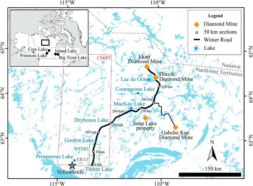
AFFILIATIONS: Mullan, Flood, and Newton—Geography, School of Natural and Built Environment,
Queen’s University Belfast, Belfast, Northern Ireland, United Kingdom; Barr—Department of Natural
Science, Manchester Metropolitan University, Manchester, United Kingdom; Galloway—Geological
Survey of Canada, Calgary, Alberta, Canada; Swindles—Geography, School of Natural and Built
Environment, Queen’s University Belfast, Belfast, United Kingdom, and Ottawa-Carleton Geoscience
Centre and Department of Earth Sciences, Carleton University, Ottawa, Ontario, Canada

T
      he Arctic has experienced warming 2–3 times greater than the long-term global mean
      trend of 0.87°C since preindustrial times (IPCC 2018), resulting in widespread shrinking
      of the cryosphere (IPCC 2019). This arctic amplification is projected to continue
throughout the twenty-first century, with a 2°C global mean temperature increase (GMTI)
projected to result in up to a 6°C warming in the Arctic (IPCC 2018). While impacts on ice
sheets and glaciers tend to capture the headlines, there are also important consequences
for infrastructure in Arctic and sub-Arctic communities, where warming temperatures
threaten the physical integrity of overland transport routes and the economies they sustain
(Meredith et al. 2019). Infrastructure built over permafrost is particularly vulnerable.
Cumulative expenses of USD 5.5 billion are projected for climate-driven damage to public
infrastructure in Alaska between 2015 and 2099 under high emissions scenarios, with one
of the top two costs associated with building damage from near-surface permafrost thaw
(Melvin et al. 2017). In a circumpolar study, Hjort et al. (2018) revealed that nearly 4 million
people and 70% of existing infrastructure in the permafrost domain lie in areas with high
potential for near-surface permafrost thaw. Winter roads, comprising seasonally frozen sea,
land, lakes, rivers, and creeks, are also under considerable threat from a warming climate.
These seasonal roads are vital for the affordable transport of heavy equipment, cargo, and fuel,
but also provide physical connections that foster social and cultural interactions among remote
communities (Chiotti and Lavender 2008; Furgal and Prowse 2008). In recent decades, climate
change has shortened the operational season of winter roads across the Canadian Arctic, and
published studies project future shortening in the James Bay region of Ontario (Hori et al. 2016,
2018); northern Manitoba and Saskatchewan (CIER 2006; Blair and Sauchyn 2010); the
Mackenzie River, Northwest Territories (ACIA 2005); and the Tibbitt to Contwoyto Winter
Road, Northwest Territories (Perrin et al. 2015; Mullan et al. 2017). One commonality in the
methods used in these previous studies is that future projections are based on regression
models developed between historic climate trends and ice thickness records. While there
is merit in this statistical approach, it lacks a process-based incorporation of the multitude
of meteorological and lake-specific parameters that influence the development of lake ice
(Dibike et al. 2012). Given this limitation, the present study applies—for the first time—a
process-based freshwater lake model to simulate the impacts of climate change on winter
roads. We do this by examining the future viability of the world’s busiest heavy-haul winter
road to GMTIs of 1.5°, 2°, and 4°C above preindustrial temperatures. We also make inferences
for the future viability of other winter roads across Arctic North America based on projected
winter warming in the region.

Study region, materials, and methods
The study region is the Tibbitt to Contwoyto Winter Road (TCWR), Canada—a seasonally
operational winter road extending from Tibbitt Lake, Northwest Territories, ~70 km east of
Yellowknife and spanning around 400 km northward across frozen lakes (85%) and overland
portages (15%) to Ekati Diamond Mine, north of Lac de Gras (JVTC 2020) (Fig. 1). The TCWR
is of considerable economic importance as the only overland transport route supplying four
mines with fuel, cement, tires, explosives, and other construction and maintenance materials

AMERICAN METEOROLOGICAL SOCIETY                                                              0 2 1 E1465
                                                                                   J U LY| 2Downloaded
                                                                        Unauthenticated                12/01/21 05:45 PM UTC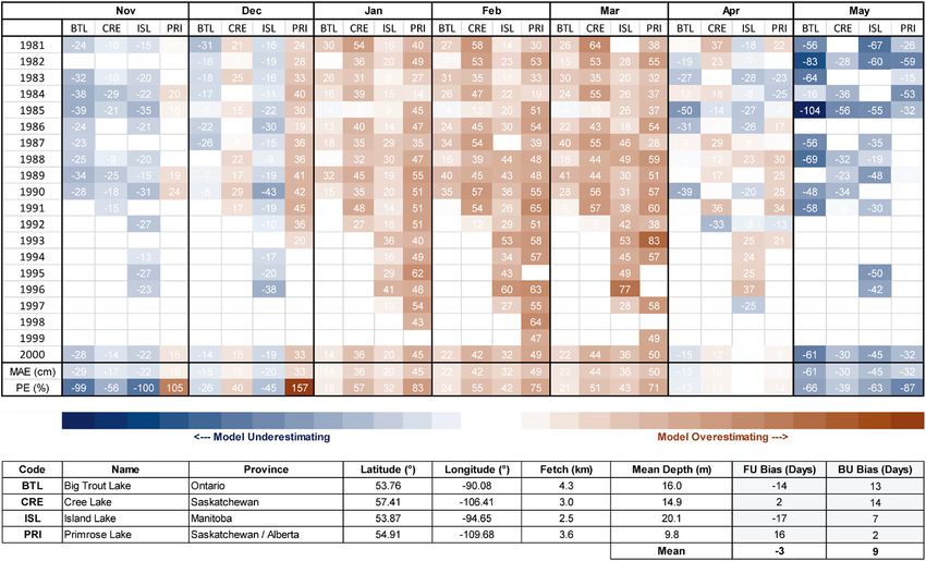
Fig. 1. The TCWR study region. The three transparent boxes show the spatial resolution of the
ERA5 (0.25° × 0.25°) and WFDEI (0.5° × 0.5°) climate observations, as well as the CMIP5 climate
model scenarios (~2.5° × 2.5° but variable from model to model). The locations of the four lakes
used for model validation are also shown in the inset map.

to a value of CAD 500 million yr−1 (Mullin et al. 2017). It is the busiest heavy-haul winter
road in the world, with more than 300,000 tonnes transported in over 10,000 loads per
year (Perrin et al. 2015). This annual haulage has, on average, been squeezed into a shorter
transport season (herein referred to as the operational season) over the past 20 years, at least
in part driven by rising air temperatures in the region (Fig. 2).

A modeling approach. We simulate ice thickness for Tibbitt Lake (62.56°N, 113.36°W) at
the southern limit of the TCWR using the FLake freshwater lake model (www.flake.igb-berlin
.de/site/download; Kirillin et al. 2011). FLake simulates the vertical temperature structure and
mixing conditions of shallow lakes (≤50 m; Huang et al. 2019). It is used as a lake parameter-
ization module in three-dimensional numerical weather prediction and climate models, but
can also run in stand-alone mode as a single-column lake model (Mironov 2008). We apply
FLake in stand-alone mode, simulating ice thickness for 20-yr simulations at a daily time
step representing 1) observed climate and 2) a set of 15 future climate scenarios. We applied
the model on a hydrological year basis—with each year beginning on 1 October and ending
on 30 September. This approach is employed to ensure model simulations begin prior to the
annual onset of ice freeze-up.

Simulations under observed climate. FLake first requires a set of lake-specific parameters.
Lake depth (6.7 m) was taken from Crann et al. (2015) and fetch (2,000 m) was approximated
by maximum lake length, measured using Google Earth. The extinction coefficient (0.6 m−1) for
water transparency was estimated from field notes associated with Galloway et al. (2010)—a

AMERICAN METEOROLOGICAL SOCIETY                                                             0 2 1 E1466
                                                                                  J U LY| 2Downloaded
                                                                       Unauthenticated                12/01/21 05:45 PM UTC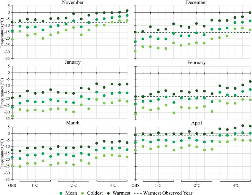
Fig. 2. Changes in the TCWR (top left) open date and (top right) close date from 2001 to 2020 (JVTC 2020),
(bottom left) season length, and (bottom right) mean annual air temperatures for Tibbitt Lake from 2001
to 2020. For the top panels and the bottom left panel, dates are expressed as days since the start of the
hydrological year on 1 Oct. Mean annual air temperatures are calculated for hydrological years, starting
on 1 Oct and ending on 30 Sep the next year.

    number representing clear water. For a 0.5° × 0.5° grid square containing Tibbitt Lake, daily
    mean temperatures, relative humidity, solar radiation, and wind speed data from 1 October
    1985 to 30 September 2005 were taken from the Watch Forcing Dataset Era Interim (WFDEI;
    Weedon et al. 2014), accessed through the Earth System Grid Federation (ESGF; https://esgf
    -node.llnl.gov/). Cloud cover data were unavailable from WFDEI and instead taken from the
    European Centre for Medium-Range Weather Forecasts (ECMWF) next-generation reanaly-
    sis (ERA5; C3S 2017), accessed through the Copernicus Climate Data Store (CDS; https://
    cds.climate.copernicus.eu/) for a 0.5° × 0.5° grid square containing Tibbitt Lake. The October
    1985 to September 2005 time period was chosen for two reasons: 1) the observational data
    are required to bias correct future climate scenarios in a later step based on its compari-
    son to a model hindcast period, with most model hindcast periods ending in 2005, and 2)
    1986–2005 is the historical baseline period used by the Intergovernmental Panel on Climate
    Change (IPCC) in their Fifth Assessment Report (AR5; IPCC 2013). FLake was run under the
    observed climate, with dates recorded when lake ice thickness exceeded 107 cm (the safe
    minimum limit for heavy-haul vehicles; Perrin et al. 2015). Since there are no measured ice
    thickness data for Tibbitt Lake, we compared measured records for four analogous shallow
    sub-Arctic Canadian lakes (locations shown in Fig. 1) with FLake simulations for the same
    lakes. The measured data were taken from Environment and Climate Change Canada
    (Environment and Climate Change Canada 2020) and were available for a minimum of 10
    years between 1981 and 2000, with FLake simulations run for the same years following
    an identical approach to input data as described above for Tibbitt Lake. Validation results
    indicate the model has a tendency to underestimate ice thickness early and late in the lake
    ice season, while observed ice thickness in the heart of the lake ice season is generally
    overestimated (appendix A, Fig. A1).

    Simulations under future climate. FLake was then run under a series of future climate sce-
    narios corresponding to GMTIs of 1.5°, 2°, and 4°C. The former two rates of warming reflect

    AMERICAN METEOROLOGICAL SOCIETY                                                               0 2 1 E1467
                                                                                        J U LY| 2Downloaded
                                                                             Unauthenticated                12/01/21 05:45 PM UTC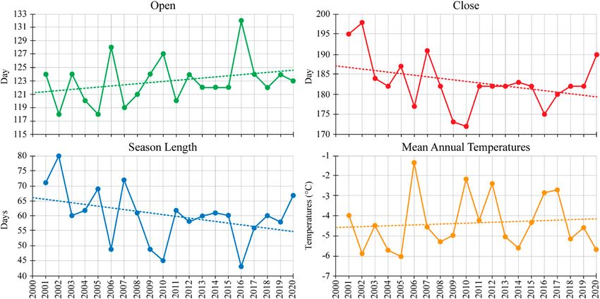
pledges made by 195 countries under the 2016 Paris Agreement (UNFCCC 2015) and are
therefore considered mitigation scenarios, whereas the latter represents something approxi-
mating a no-mitigation scenario—a rate of warming evaluated as being as likely as not to be
exceeded by the end of the twenty-first century under the highest representative concentra-
tion pathway (RCP) 8.5 (IPCC 2013). To account for Arctic amplification, we examined how
the selected GMTIs corresponded to warming in the study region and found that 1.5°, 2°, and
4°C equated to 2.9°, 3.9°, and 7.8°C (appendix B). These are herein referred to as regional
mean temperature increases (RMTIs). For each RMTI, we short-listed five climate scenarios
(n = 15) from an initial pool of 82 available, based on how closely they compared to observa-
tions at a monthly temporal resolution for a hindcast period from 1986 to 2005 (appendix
C, Table C1). Daily mean temperatures from the 15 model scenarios were then downloaded
from the ESGF and CDS for the grid square containing Tibbitt Lake. All scenarios are part of
the Coupled Model Intercomparison Project (CMIP5; Taylor et al. 2012), forced with RCP8.5
(van Vuuren et al. 2011)—a high radiative forcing scenario necessary to capture RMTIs up to
7.8°C. For each scenario, we extracted the 20-yr future time period when projected tempera-
tures reached 2.9°, 3.9°, and 7.8°C above preindustrial temperatures. Projected temperatures
were bias corrected using the change factor methodology used in Ho et al. (2012) (appendix
D). Only temperatures were modified from the baseline FLake simulations, with the other
meteorological parameters left constant. This reflects the dominant role that air temperatures
play in changing lake ice conditions (Brown and Duguay 2010), but also the fact that some
of the other meteorological parameters are unavailable from many of the selected climate
models. FLake was then run under each projected climate scenario and the dates recorded
when lake ice thickness exceeded the 107-cm threshold. The projected operational season of
the TCWR for each model was adjusted to reflect the difference between the baseline simula-
tions and the historical operational season of the TCWR (JVTC 2020) (appendix E). We also
downloaded temperatures for the period 1 October 2000–31 September 2020 from ERA5
(C3S 2017) to capture years post-2005 and allow us to relate these to the TCWR operational
season observations. Present and future operational season length was then color coded in
a traffic light system based on an economic analysis conducted by Perrin et al. (2015). Green
indicates ≥50 days, a viable season; amber indicates 45–49 days, an “adaptive scenario”
where flexible scheduling is required to meet season demands at a high cost of around USD
1.57 million yr−1; and red indicates
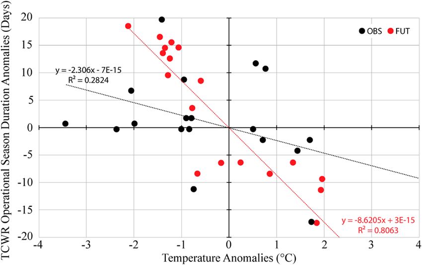
Fig. 3. TCWR operational season as observed for the present (mean of 2001–20 observations
taken from JVTC 2020) (n = 1) and simulated by FLake for the future under 15 climate scenarios
corresponding to a GMTI of 1.5°C (n = 5), 2°C (n = 5), and 4°C (n = 5). The mean of the 20-yr
observations/simulations is shown in medium blue, while the year with the shortest (longest)
season is shown in dark (light) blue. Also shown is the operational season length (days) for the
mean, shortest, and longest years in a traffic light color system following the scenarios outlined
in Perrin et al. (2015): ≥50 days = green (viable), 45–49 days = amber (viable with costly adapta-
tion),
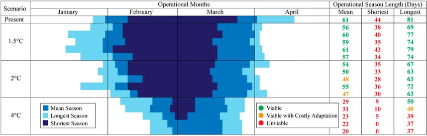
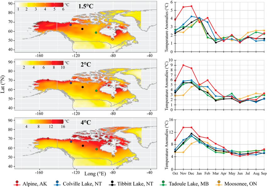
Fig. 4.(left) Mean projected December temperature anomalies for the northern half of North America. Temperature
anomalies are expressed as the mean of the models analyzed in this study at a GMTI of 1.5°, 2°, and 4°C from the mean
1986–2005 observed period. (right) Temperature anomalies (calculated in the same way as above) for each month of the
year for five winter roads in North America (including the TCWR, as represented by Tibbitt Lake, NT). Two-letter state/
province/territory codes are used for the five winter road locations—AK: Alaska; MB: Manitoba; NT: Northwest Territories;
ON: Ontario.

            period of winter roads—essential for providing a more climatically favorable construction
            period and contributing to earlier opening dates. When warming of the magnitude projected
            here occurs during this preconditioning period, it is unsurprising that a considerable delay
            in the opening of the TCWR follows. Figure 4 reveals this pattern could be expected to an
            even larger degree across much of the rest of Arctic North America, with a GMTI of 1.5°, 2°,
            and 4°C resulting in regional December warming in excess of 5°, 8°, and 15°C across parts
            of the Prudhoe Bay coast of Alaska, the Northwest Territories, Nunavut, and the Hudson Bay
            coastal regions of Manitoba, Ontario, and Quebec. With a number of prominent winter roads
            in these regions, a widespread shift toward costly adaptation or route closure seems likely.
               The levels of winter warming projected here—in places over 3 times the global average—are
            consistent with projections for the Arctic by the end of the twenty-first century (IPCC 2013,
            2019). These high rates of warming can be explained by a projected continuation of arctic
            amplification, where observed records in recent decades show a warming signal that has been
            strongest over the Arctic Ocean in autumn and winter (Cohen et al. 2014; Horton et al. 2015).
            A number of mechanisms are thought to be responsible for enhanced sensitivity to warming
            in the Arctic, but chief among them is the change in sea ice albedo owing to the stark dif-
            ference in reflective properties of an ice-free ocean and snow-covered sea ice surfaces (~7%

            AMERICAN METEOROLOGICAL SOCIETY                                                              0 2 1 E1470
                                                                                               J U LY| 2Downloaded
                                                                                    Unauthenticated                12/01/21 05:45 PM UTC
vs 80% reflectance, respectively; Cohen et al. 2019). This likely explains the high degree of
warming, particularly along the Arctic coastal regions in autumn and winter (Fig. 4). Other
more localized arctic amplification mechanisms may contribute to enhanced autumn and
winter warming in the study region, located ~500 km south of the Arctic coast. Local forc-
ings include snow, cloud, and ice insulation feedbacks (Kwok et al. 2009; Lee et al. 2011;
Yang and Magnusdottir 2018), while increased vegetation over Arctic land contributes to
surface darkening at high latitudes (Overland et al. 2015). It is thought that local and remote
forcing mechanisms may interact and amplify one another (Yang and Magnusdottir 2018),
meaning some combination of all the above factors is likely at play in amplifying warming in
the wider TCWR region. Attribution studies indicate that increasing anthropogenic greenhouse
gases play a vital role in driving Arctic surface temperature increases (Fyfe et al. 2013;
Najafi et al. 2015), leading to a high confidence in projections of further Arctic warming
(Overland et al. 2019).
Interannual variability. The interannual variability within the 20-yr observations and simu-
lation periods reveals that mean patterns are subject to considerable divergence from year to
year, as shown in Fig. 5. During the observed period, the TCWR opened as late as 9 February in
2016 (9 days later than the mean), while it closed as early as 21 March in 2010 (11 days earlier
than the mean). As seen in Fig. 5 and in Fig. 2, shortened seasons are often associated with
anomalously warm years, partly due to large-scale teleconnections that correlate most strongly
with Canadian climate during winter (Bonsal and Shabbar 2011). Anomalous heating in the
Eastern tropical Pacific associated with El Niño results in a positive Pacific–North American
(PNA) pattern over North America (Wallace and Gutzler 1981) and consequently warmer
than average temperatures from late autumn to early spring (Shabbar and Khandekar 1996).
The two shortest operational seasons on record (2010: 46 days; and 2016: 44 days) follow
two of the strongest El Niño events in recent decades: 2009/10 and 2015/16 (Timmermann
et al. 2018). Shorter op-
erational seasons in some
cases may also be associ-
ated with increased winter
storminess. Major storms
with high wind speeds and
blowing snow can cause
temporary closures on the
road, as occurred in March
2012 (Perrin et al. 2015).
Where anomalously warm or
stormy winters cause the ice
to break open in a “blowout”
(Perrin et al. 2015), winter
roads may shut for mainte-
nance or may even close for
the season. The short 50-day
season in 2006 occurred in Fig. 5. November–April mean temperature (°C) and TCWR seasonal duration
such a way, with a blowout (days) anomalies for the Tibbit Lake region of the TCWR. Anomalies for
on Waite Lake late in the each year of the 20-yr observed record/model simulations are expressed
as changes relative to the mean of that same 20-yr period. Black points
season (14 March) before the
represent observations (OBS) for 2000–20, and red points represent the
season was complete (Perrin most extreme model simulation (FUT) under a 4°C GMTI—in this case for
et al. 2015). Consequently, 2079–99—the 20-yr period when temperatures first rise the RMTI equivalent
approximately 1,200 loads of 4°C GMTI above preindustrial temperatures.
AMERICAN METEOROLOGICAL SOCIETY 0 2 1 E1471
J U LY| 2Downloaded
Unauthenticated 12/01/21 05:45 PM UTCwere flown into mines in the summer and autumn of 2006 at a cost of CAD 100–150 million
(Perrin et al. 2015). A poleward shift in extratropical cyclone activity is projected to result
in increased atmospheric moisture and greater winter precipitation over the northern half of
North America (Christensen et al. 2013). This indicates the clear future potential for an increase
in blowing snow and hazardous blizzards that further threaten the operational season of the
TCWR. Conversely, longer operational seasons are typically associated with colder than aver-
age years. For example, the longest operational season on record (26 January–16 April 2002:
81 days) occurred when 2001/02 winter and early 2002 spring temperatures were consider-
ably colder than average. Cooler years are typically associated with modes of variability in
opposite phases to anomalously warm years. A switch toward La Niña events and a negative
phase of the PNA are associated with earlier freeze-up and later breakup of lake and river
ice across much of Canada (Bonsal et al. 2006). Figure 5 shows that interannual variability
in temperatures and the winter road operational season are projected to continue in future,
indicating that natural variability will continue to result in considerable year to year diver-
gence from the mean. Figure 3 shows that the year with the longest projected operational sea-
son under 1.5°C (69–79 days) and 2°C (63–72 days) is always longer than the mean observed
season (61 days) and reflective of a viable season in the Perrin et al. (2015) classification. In
addition, Fig. 3 shows that the mean projected operational season is always longer at 1.5°C
(56–61 days) and 2°C (47–55 days) than it is during the shortest year of the observed record
(44 days). Figure 6 reveals the reason for this, as temperature anomalies during the warm-
est observed year are higher than the mean temperature anomalies for 1.5° and 2°C for all
months under most future scenarios (note this refers to the warmest observed year out of 20
simulated years, where the actual year may differ between months). Furthermore, the year
with the longest projected operational season at 4°C (37–50 days) is for two models greater
than the shortest observed operational season (44 days). Figure 6 again shows why, since
the year with coldest projected temperatures under 4°C is colder than the warmest observed
year during January–April. In this sense, greater future variability may offer hope that colder
than average years could permit some fully operational seasons, even when the mean sug-
gests otherwise. For example, under the least extreme 2°C model—where a mean operational
season of 55 days is projected—there are 12 years out of 20 where a fully viable season up to
the longest year of 72 days is projected.
However, greater future variability also means there are several years that fall below
the mean. The same 2°C scenario referred to above has a shortest season length of 36 days
and eight out of 20 years that fall below the 50-day threshold. Considering the shortened
50-day season and associated high costs in 2006, it is clear that scenarios such as the one
identified above do not lend support to a viable TCWR without at least considerable adap-
tation. Even under 1.5°C scenarios, where the mean operational seasons of all five models
exceed the 50-day threshold, shortest seasons lie below 40 days—with several years among
the 20-year projections falling below the viable threshold. For example, under the least
extreme 1.5°C model—where the mean season length is 61 days—there are still four years
out of 20 where the operational season is less than 50 days. Falling short of a viable season
length at a frequency of once every five years may raise important questions among plan-
ners about the long-term viability of the TCWR. That outlook becomes even bleaker when
we examine the most extreme 1.5° and 2°C scenarios, with seven out of 20 years below the
50-day threshold for the former, and 11 years for the latter. At 4°C, the TCWR is unequivo-
cally unviable. Three out of five models under the 4°C scenarios project all 20 years to fall
below the 50-day threshold, with the other two models projecting only one or two years,
respectively, above this threshold. As shown in Fig. 6, temperatures rising above freezing
in November and April under these scenarios indicates why such large reductions in the
operational season are simulated.
AMERICAN METEOROLOGICAL SOCIETY 0 2 1 E1472
J U LY| 2Downloaded
Unauthenticated 12/01/21 05:45 PM UTCFig. 6. November–April temperatures at Tibbitt Lake as observed (OBS) for the present (n = 1) and simulated
for the future under 15 climate scenarios corresponding to a GMTI of 1.5°C (n = 5), 2°C (n = 5), and 4°C
(n = 5). The mean of the 20-yr observations/simulations is shown in medium green, while the year with
the coldest (warmest) temperatures for each particular month is shown in light (dark) green. The dashed
line represents observed temperatures during the warmest year (mean of November–April).
Adaptation. Before considering costly large-scale adaptation options, there are first adap-
tations to present-day practices that may help ensure the TCWR remains viable for longer.
Sladen et al. (2020) investigated threshold requirements for the initiation of winter road
operations along the TCWR and found that the current practice of planning construction
by calendar dates rather than by evaluation of air-freezing indices results in a conservative
approach to the start of the construction season. In the interests of “winning back” some time
as the climate reduces the length of the operational season, it may be necessary to adapt a
more methods-based approach to the dates of winter road construction by installing equip-
ment to calculate freezing indices or measure frozen ground depths and temperatures. It is
also clear, however, that such an approach incurs expense, logistical challenges, and issues
with mobilizing equipment and personnel at short notice (Sladen et al. 2020). Amending the
nature of annual haulage on the TCWR may also represent a low-cost adaptation measure in
the face of shortening operational seasons. For winter roads linking remote communities, the
desire is to ensure as long a season as possible. This is not the case for the TCWR, where the
goal is to ensure specified tonnages of materials to mines are provided during the operational
season. Where the season length is reduced, lost service may be recovered by increasing the
number of daily loads (Perrin et al. 2015). We see evidence of this in the historical records
(Table 1)—years with a reduced operational season but higher freight statistics than years
AMERICAN METEOROLOGICAL SOCIETY 0 2 1 E1473
J U LY| 2Downloaded
Unauthenticated 12/01/21 05:45 PM UTCTable 1. Historical operational season statistics for the TCWR (JVTC 2020).
Year Open date Close date Duration (days) No. of Loads Tonnes
2001 1 Feb 13 Apr 72 7,981 245,586
2002 26 Jan 16 Apr 81 7,735 256,915
2003 1 Feb 2 Apr 61 5,243 198,818
2004 28 Jan 31 Mar 63 5,091 179,144
2005 26 Jan 5 Apr 70 7,607 252,533
2006 4 Feb 26 Mar 50 6,841 177,674
2007 27 Jan 9 Apr 73 10,922 330,002
2008 29 Jan 7 Apr 62 7,484 245,585
2009 1 Feb 25 Mar 50 5,377 173,195
2010 4 Feb 24 Mar 46 3,508 120,020
2011 28 Jan 31 Mar 63 6,832 239,000
2012 1 Feb 28 Mar 59 6,551 210,188
2013 30 Jan 31 Mar 61 6,017 223,206
2014 30 Jan 1 Apr 62 7,069 243,928
2015 30 Jan 31 Mar 61 8,915 305,215
2016 9 Feb 24 Mar 44 8,766 262,261
2017 1 Feb 29 Mar 57 8,241 279,484
2018 1 Feb 31 Mar 61 8,209 303,725
2019 1 Feb 31 Mar 59 7,489 257,176
2020 31 Jan 8 Apr 68 7,072 230,497
with a longer season. For example, 2016 ranks third out of 20 years for highest number of
loads (8,766) and tonnes transported (262,261), despite being the shortest operational year
(44 days) on record. This clearly shows there is some scheduling flexibility that can help offset
a shortened operational season. The limiting factor in this scenario is the number of trucks
and drivers available (Perrin et al. 2015). Increasing their provision to facilitate maximizing
the daily use of the TCWR may therefore avoid more costly adaptation. The above adaptations
may help under the less extreme scenarios highlighted in this study, but larger-scale higher-
cost alternatives may be needed under more extreme scenarios. Options already considered
for the TCWR include construction of an all-season gravel-surface overland route along the
most vulnerable southern portion; construction of a deep sea port at Bathurst Inlet, Nunavut,
with a road to the mines across colder Arctic tundra; and construction of 600 km of power
lines to expand hydroelectric power and reduce reliance of the mines on diesel—the most
transported commodity in the TCWR (Perrin et al. 2015). If pledges to reduce greenhouse gas
emissions are not met, there may be little alternative but to implement one or more of these
measures to protect economic activity in the region.
Conclusions, limitations, and future work.
Unlike previous studies, use of a process-based freshwater lake model has allowed us
to incorporate more of the factors influencing the development and evolution of lake ice
along the TCWR. Despite this, there are a number of limitations that must be considered
when interpreting the results. FLake has been found to overestimate ice thickness (e.g.,
Kheyrollah Pour et al. 2012)—a trend clearly evident in our validation (Fig. A1) during the
peak cold season between January and March. We also identified an underestimation of ice
thickness in November/December and in April/May, corresponding with slightly later than
observed freeze-up (by 3 days on average) and earlier breakup (by 9 days on average). These
freeze-up/breakup trends are similar to some studies (e.g., Kheyrollah Pour et al. 2012;
AMERICAN METEOROLOGICAL SOCIETY 0 2 1 E1474
J U LY| 2Downloaded
Unauthenticated 12/01/21 05:45 PM UTCRontu et al. 2019) and opposite in sign to others (e.g., Yang et al. 2013; Kourzeneva 2014;
Pietikäinen et al. 2018). Timing of overestimation and underestimation in our valida-
tion results likely points to difficulties in simulating the accumulation of snow on lake ice
(Rontu et al. 2019). FLake does not account for the insulating effect of snow, meaning ice is
able to thicken more rapidly but also melt faster without snow buffering ice from the cold air
above (Jeffries and Morris 2006). Although provision is made to model parametrically the
evolution of snow cover above lake ice in FLake, the model has not been sufficiently tested
in this regard and is highlighted as an area requiring development (FLake 2020). It is not
possible to quantify in days the potential impact this limitation has on the operational season
length of the TCWR, but we highlight this as a particular point of caution when interpreting
the projected dates shown in Fig. 3. The daily time step may be too temporally coarse to take
account of important processes relating to ice formation, including low wind speeds and calm
events creating the potential for complete lake freeze within hours (Bernhardt et al. 2012).
This highlights another important issue—only air temperatures were modified in the future
simulations owing to data availability. This limits the reliability of future projections since
interactions with other changing meteorological properties including wind speed are essential
components in ensuring vertical heat transfer is sufficient to cool surface water temperatures
to 0°C (Leppäranta 2010; Nõges and Nõges 2014). Perturbing other meteorological variables
in the model in addition to mean temperatures would build a fuller picture of the impacts
of climate change on the TCWR. No ice thickness measurements were available for Tibbitt
Lake, so it is not possible to fully evaluate model performance for the lake simulated in this
study. Future studies could also build on our progress by accounting for the ~15% of the
TCWR route crossing overland portages, which primarily comprise permafrost peatlands
(Sladen et al. 2020). With rapid thawing of permafrost peatlands in the Canadian Arctic
(Swindles et al. 2015; Sim et al. 2019), it is currently unclear if these sections of the TCWR
are more or less vulnerable to warming than lakes. Finally, a continental or hemispheric-scale
study simulating the impacts of climate change on other winter roads across the high latitudes,
beyond the inferences we have made, would be highly valuable. In the meantime, our work
represents a considerable advance on previous studies and highlights the escalating threat
that climate change poses to the future viability of the TCWR and most likely other North
American winter roads. The identification of a tipping point at 2°C GMTI illustrates that the
actions of current and future generations in cutting greenhouse gas emissions is critical to
the future viability of winter roads and the vital role they provide in building economies and
linking communities in the northern high latitudes.
Acknowledgments. The authors acknowledge helpful feedback received on the manuscript from Steve
Grasby, Geological Survey of Canada.
Data availability statement. References to the datasets used in this study and the web addresses for
the data repositories they were downloaded from can be found in the “Study region, materials, and
methods” section (and in appendixes A and B). All data are freely and openly available.
Appendix A: FLake Model Validation
Ice thickness data for four lakes in Canada were downloaded from Environment and Climate
Change Canada. We selected the four lakes following a careful screening process that
started by examining all available lake ice records from Environment and Climate Change
Canada and including those lakes that fulfilled the following criteria: 1) latitude > 52.5°
(to ensure lakes are within 10° of the study lake); 2) >10 years of data between 1981 and
2000 (to correspond with the modeling time period for the study lake); and 3) lakes with
a mean depth < 50 m (as determined from the Global Lake Database)—note 50-m depth is
AMERICAN METEOROLOGICAL SOCIETY 0 2 1 E1475
J U LY| 2Downloaded
Unauthenticated 12/01/21 05:45 PM UTCconsidered the upper limit of suitability for FLake modeling. This generated a validation
database comprising four lakes—the details of which are provided in Fig. A1. Measurements
for these four lakes exist at approximately a weekly temporal resolution and were mea-
sured to the nearest centimeter using a special auger kit or hot wire ice thickness gauge
(Environment and Climate Change Canada 2020). FLake simulations were run from 1 October
1981 to 30 September 2000 and were then compared to the observed ice thickness records by
extracting modeled ice thickness only for the precise dates where measured data existed during
the 19-yr comparison period. The two sets of data were then compared for the (inclusive)
months November–May, with the absolute error, mean absolute error, and percentage error
calculated to determine the degree to which the model under or overestimated ice thickness
during these months (Fig. A1). We also downloaded observed freeze-up and breakup dates
for each validation lake from the Global Lake and River Ice Phenology Database Version 1
(Benson et al. 2020) and compared these records with FLake simulated freeze-up and breakup
dates for the same years as the data used to calculate absolute error (Fig. A1).
Fig. A1. Absolute error (observed ice thickness minus modeled ice thickness) for four analogous shallow sub-Arctic Canadian
lakes (the details of which are provided in the table part of the figure) covering a minimum of 10 years during the period
1981–2000. Results are provided on a monthly basis, with mean absolute error (MAE) calculated for all years with mea-
surements and percentage error (PE) calculated as relative error multiplied by 100. Also provided in the table part of the
figure is freeze-up (FU) bias and breakup (BU) bias—calculated as observed FU/BU minus FLake simulated FU/BU for each
lake across the same years as the data used to calculate absolute error in the main part of the figure. Negative (positive)
numbers indicate FU/BU is simulated later (earlier) than observed.
Appendix B: Calculating RMTIs
To calculate RMTIs for the study area, monthly mean temperatures were downloaded from
KNMI Climate Explorer (https://climexp.knmi.nl/). Historical monthly mean temperatures for the
AMERICAN METEOROLOGICAL SOCIETY 0 2 1 E1476
J U LY| 2Downloaded
Unauthenticated 12/01/21 05:45 PM UTCperiod 1986–2005 were subtracted from the 2006–2100 period forced with RCP8.5 for the
mean of all CMIP5 models and ensembles. This was done for the global average (resulting
in 2.0°C) and subsequently for the grid square containing Tibbitt Lake (resulting in 3.9°C).
This global-to-regional ratio of 2.0:3.9 was subsequently used to correct GMTIs of 1.5°, 2°,
and 4°C by simply dividing 3.9 by 2.0 and multiplying by the relevant GMTI. This produced
RMTIs of 2.9°, 3.9°, and 7.8°C. We deducted 0.6 from each RMTI to reflect the fact that the
1986–2005 period was 0.6°C warmer than preindustrial temperatures, and then calculated the
mean 20-yr period when temperatures were 2.3°, 3.3°, and 7.2°C higher than the 1986–2005
hindcast period for each model.
Appendix C: Short-listing climate models
We downloaded all available CMIP5 models and ensembles at a monthly temporal resolution
under RCP8.5 (n = 82) for the grid square containing Tibbitt Lake. For all 82 scenarios, we
calculated the root-mean-square error (RMSE) from the difference between the 1986–2005
historical temperatures for that scenario and the 1986–2005 observed temperatures for Tibbitt
Lake. The 82 scenarios were ranked by their RMSE and the top five for each GMTI short-listed
for subsequent FLake modeling. In several cases, a different 20-yr future time period from
the same scenario was used among the final 15 scenarios. The full list of selected scenarios
and extracted time periods is given in Table C1.
Table C1. All 15 short-listed scenarios as used for FLake modeling. Root-mean-square error (RMSE)
is provided, along with the extracted years for each scenario. Twenty-year time periods were taken
from 1 Oct on the start year to 30 Sep on the end year to conform to the temporal basis of FLake
modeling and represent the 20-yr mean period when temperatures first exceed the RMTI associated
with each of the three GMTIs.
Model ensemble RMSE 1.5°C 2°C 4°C
IPSL-CM5A-LR r1i1p1 1.16 2033–53 2039–59 2074–94
ICHEC EC-Earth r2i1p1 1.42 2029–49 2047–67
NOAA GFDL-ESM2G r1i1p1 1.52 2037–57 2058–78
CSIRO-QCCCE CSIRO-Mk3-6-0 r9i1p1 1.54 2031–51 2043–63
IPSL-CM5A-LR r4i1p1 1.37 2027–47
CSIRO-QCCCE CSIRO-Mk3-6-0 r8i1p1 1.46 2048–68
IPSL-CM5A-LR r3i1p1 1.78 2075–95
MIROC5 r2i1p1 1.82 2066–86
MIROC5 r3i1p1 1.90 2069–89
CSIRO-QCCCE CSIRO-Mk-3-6-0 r1i1p1 1.92 2079–99
Appendix D: Bias correction
Daily temperature projections for each scenario were bias corrected using a change factor
(CF) methodology that uses observed daily variability and changes the mean and daily vari-
ance as simulated by the model (e.g., Arnell et al. 2003; Gosling et al. 2009). Outlined in
Ho et al. (2012), this method takes the form:
σTRAW
TCF (t ) =TRAW + OREF (t ) – TREF ,
σTREF
where TRAW represents daily raw model output for the future period, TREF represents daily raw
model output for the historical period, OREF represents daily observed output, time t repre-
sents a daily time step, the bar above a symbol denotes the mean, and σ represents standard
deviation.
AMERICAN METEOROLOGICAL SOCIETY 0 2 1 E1477
J U LY| 2Downloaded
Unauthenticated 12/01/21 05:45 PM UTCAppendix E: Operational season adjustment
Projected operational season dates were adjusted using the following equation:
D
DAdjOBS = REF ( DFUT – DOBS ),
DOBS
where DAdjOBS represents adjusted projected operational season dates, DREF represents projected
operational dates for the baseline simulations, DOBS represents operational dates from historical
records (2001–20), and DFUT represents projected operational dates from future simulations.
AMERICAN METEOROLOGICAL SOCIETY 0 2 1 E1478
J U LY| 2Downloaded
Unauthenticated 12/01/21 05:45 PM UTCReferences
ACIA, 2005: Arctic Climate Impact Assessment. Cambridge University Press, 1020 pp. Galloway, J. M., A. Macumber, R. T. Patterson, H. Falck, T. Hadlari, and E. Madsen,
Arnell, N. W., D. A. Hudson, and R. G. Jones, 2003: Climate change scenarios from 2010: Paleoclimatological assessment of the southern northwest territories
a regional climate model: Estimating change in runoff in southern Africa. J. and implications for the long-term viability of the Tibbitt to Contwoyto Winter
Geophys. Res., 108, 4519–4535, https://doi.org/10.1029/2002JD002782. Road, Part I: Core collection. NWT Open Rep. 2010-002, Northwest Territo-
Benson, B., J. Magnuson, and S. Sharma, 2020: Global lake and river ice phenol- ries Geoscience Office, 21 pp., https://carleton.ca/timpatterson/wp-content/
ogy database, version 1. National Snow and Ice Data Center, accessed 20 uploads/NWT_OR_2010-002-1.pdf.
March 2021, https://doi.org/10.7265/N5W66HP8. Gosling, S., G. McGregor, and J. Lowe, 2009: Climate change and heat-related
Bernhardt, J., C. Engelhardt, G. Kirillin, and J. Matschullat, 2012: Lake ice phenology mortality in six cities Part 2: Climate model evaluation and projected impacts
in Berlin-Brandenburg from 1947–2007: Observations and model hindcasts. from changes in the mean and variability of temperature with climate change.
Climatic Change, 112, 791–817, https://doi.org/10.1007/s10584-011-0248-9. Int. J. Biometeor., 53, 31–51, https://doi.org/10.1007/s00484-008-0189-9.
Blair, D., and D. Sauchyn, 2010: Winter roads in Manitoba. The New Normal: Hawkins, E., T. M. Osborne, C. Kit Ho, and A. J. Challinor, 2013: Calibration and
The Canadian Prairies in a Changing Climate, D. Sauchyn, H. Diaz, and S. bias correction of climate projections for crop modelling: An idealised case
Kulshreshtha, Eds., CPRC Press, 322–325. study over Europe. Agric. For. Meteor., 170, 19–31, https://doi.org/10.1016/j.
Bonsal, B., and A. Shabbar, 2011: Large-scale climate oscillations influencing agrformet.2012.04.007.
Canada, 1900–2008. Canadian Biodiversity: Ecosystem Status and Trends Hjort, J., and Coauthors, 2018: Degrading permafrost puts Arctic infrastructure at
2010, Tech. Thematic Rep. 4, Canadian Councils of Resource Ministers, risk by mid-century. Nat. Commun., 9, 5147, https://doi.org/10.1038/s41467-
20 pp., https://biodivcanada.chm-cbd.net/sites/biodivcanada/files/2018- 018-07557-4.
02/974No.4_Climate%20Oscillations%20April%202011_E.pdf. Ho, C. K., D. B. Stephenson, M. Collins, C. A. T. Ferro, and S. J. Brown, 2012:
—, T. D. Prowse, C. R. Duguay, and M. P. Lacroix, 2006: Impacts of large-scale Calibration strategies: A source of additional uncertainty in climate change
teleconnections on freshwater-ice break/freeze-up dates over Canada. J. projections. Bull. Amer. Meteor. Soc., 93, 21–26, https://doi.org/10.1175/
Hydrol., 330, 340–353, https://doi.org/10.1016/j.jhydrol.2006.03.022. 2011BAMS3110.1.
Brown, L. C., and C. R. Duguay, 2010: The response and role of ice cover in Hori, Y., W. A. Gough, K. Butler, and L. J. S. Tsuji, 2016: Trends in the seasonal length
lake-climate interactions. Prog. Phys. Geogr., 34, 671–704, https://doi. and opening dates of a winter road in the western James Bay region, Ontario,
org/10.1177/0309133310375653. Canada. Theor. Appl. Climatol., 129, 1309–1320, https://doi.org/10.1007/
C3S, 2017: ERA5: Fifth generation of ECMWF atmospheric reanalyses of the glob- s00704-016-1855-1.
al climate. Copernicus Climate Change Service Climate Data Store, accessed —, V. Y. S. Cheng, W. A. Gough, J. Y. Jien, and L. J. S. Tsuji, 2018: Implications
19 May 2020, https://cds.climate.copernicus.eu/cdsapp#!/home. of projected climate change on winter road systems in Ontario’s Far North,
Chiotti, Q., and B. Lavender, 2008: Ontario. From Impacts to Adaptation: Canada Canada. Climatic Change, 148, 109–122, https://doi.org/10.1007/s10584-
in a Changing Climate 2007, D. S. Lemmen et al., Eds., Government of Canada, 018-2178-2.
227–274. Horton, R., N. C. Johnson, D. Singh, D. L. Swain, B. Rajaratnam, and N. S. Diffenbaugh,
Christensen, J. H., and Coauthors, 2013: Climate phenomena and their relevance 2015: Contribution of changes in atmospheric circulation patterns to extreme
for future regional climate change. Climate Change 2013: The Physical temperature trends. Nature, 522, 465–469, https://doi.org/10.1038/nature14550.
Science Basis, T. F. Stocker et al., Eds., Cambridge University Press, 1217–1308. Huang, A., and Coauthors, 2019: Evaluating and improving the performance
CIER, 2006: Climate change impacts on ice, winter roads, access trails, and Manitoba of three 1-D lake models in a large deep lake of the central Tibetan
First Nations. Accessed 16 June 2012, www.nrcan.gc.ca/earthsciences/projdb Plateau. J. Geophys. Res. Atmos., 124, 3143–3167, https://doi.org/10.1029
/pdf/187b_e.pdf. /2018JD029610.
Cohen, J., and Coauthors, 2014: Recent Arctic amplification and extreme mid- IPCC, 2013: Summary for policymakers. Climate Change 2013: The Physical Sci-
latitude weather. Nat. Geosci., 7, 627–637, https://doi.org/10.1038/ngeo2234. ence Basis, T. E. Stocker et al., Eds., Cambridge University Press, 1–29, www.
—, and Coauthors, 2019: Divergent consensuses on Arctic amplification influ- ipcc.ch/report/ar5/wg1/.
ence on midlatitude severe winter weather. Nat. Climate Change, 10, 20–29, —, 2018: Summary for policymakers. Global Warming of 1.5°C, V. Masson-
https://doi.org/10.1038/S41558-019-0662-Y. Delmotte et al., Eds., 24 pp., www.ipcc.ch/site/assets/uploads/sites/2/2019/05/
Crann, C. A., R. T. Patterson, A. L. Macumber, J. M. Galloway, H. M. Roe, M. Blaauw, SR15_SPM_version_report_LR.pdf.
G. T. Swindles, and H. Falck, 2015: Sediment accumulation rates in subarctic —, 2019: Summary for policymakers. Ocean and Cryosphere in a Changing Cli-
lakes: Insights into age-depth modeling from 22 dated lake records from the mate, H.-O. Pörtner et al., Eds., IPCC, 36 pp., www.ipcc.ch/site/assets/uploads/
Northwest Territories, Canada. Quat. Geochronol., 27, 131–144, https://doi. sites/3/2019/11/03_SROCC_SPM_FINAL.pdf.
org/10.1016/j.quageo.2015.02.001. Jeffries, M. O., and K. Morris, 2006: Instantaneous daytime conductive heat flow
Dibike, Y., T. Prowse, B. Bonsal, L. de Rham, and T. Saloranta, 2012: Simulation of through snow on lake ice in Alaska. Hydrol. Processes, 20, 803–815, https://
North American lake-ice cover characteristics under contemporary and future doi.org/10.1002/hyp.6116.
climate conditions. Int. J. Climatol., 32, 695–709, https://doi.org/10.1002/ Jensen, O. P., 2007: Spatial analysis of ice phenology trends across the Laurentian
joc.2300. Great Lakes region during a recent warming period. Limnol. Oceanogr., 52,
Environment and Climate Change Canada, 2020: Ice thickness data. Accessed 2013–2026, https://doi.org/10.4319/lo.2007.52.5.2013.
18 April 2020, www.canada.ca/en/environment-climate-change/services/ice- JVTC, 2020: Tibbitt to Contwoyto Winter Road. Joint Venture Trucking Commit-
forecasts-observations/latest-conditions/archive-overview/thickness-data.html. tee, accessed 23 April 2020, https://jvtcwinterroad.ca/wp-content/uploads
FLake, 2020: Useful hints. Accessed 24 December 2020, https://flake.igb-berlin. /2021/01/2021-Winter-Road-Poster.pdf.
de/site/download. Kheyrollah Pour, H., C. R. Duguay, A. Martynov, and L. C. Brown, 2012: Simulation
Furgal, C., and T. Prowse, 2008: Northern Canada. From Impacts to Adaptation: of surface temperature and ice cover of large northern lakes with 1-D models:
Canada in a Changing Climate 2007, D. S. Lemmen et al., Eds., Government A comparison with MODIS satellite data and in situ measurements. Tellus,
of Canada, 57–118. 64A, 17614, https://doi.org/10.3402/TELLUSA.V64I0.17614.
Fyfe, J. C., and Coauthors, 2013: One hundred years of Arctic surface tempera- Kirillin, G., J. Hochschild, D. Mironov, A. Terzhevik, S. Golosov, and G. Nützmann,
ture variation due to anthropogenic influence. Sci. Rep., 3, 2645, https://doi. 2011: FLake-Global: Online lake model with worldwide coverage. Environ.
org/10.1038/srep02645. Modell. Software, 26, 683–684, https://doi.org/10.1016/j.envsoft.2010.12.004.
AMERICAN METEOROLOGICAL SOCIETY 0 2 1 E1479
J U LY| 2Downloaded
Unauthenticated 12/01/21 05:45 PM UTCKourzeneva, E., 2014: Assimilation of lake water surface temperature observa- future predictions. Ann. Glaciol., 46, 443–451, https://doi.org/10.3189
tions with extended Kalman filter. Tellus, 66A, 21510, https://doi.org/10.3402/ /172756407782871431.
tellusa.v66.21510. Rontu, L., K. Eerola, and M. Horttanainen, 2019: Validation of lake surface state
Kwok, R., and Coauthors, 2009: Thinning and volume loss of the Arctic Ocean sea in the HIRLAM v.7.4 numerical weather prediction model against in situ
ice cover: 2003–2008. J. Geophys. Res., 114, C07005, https://doi.org/10.1029 measurements in Finland. Geosci. Model Dev., 12, 3707–3723, https://doi.
/2009JC005312. org/10.5194/gmd-12-3707-2019.
Lee, S., T. T. Gong, N. C. Johnson, S. B. Feldstein, and D. Pollard, 2011: On the pos- Shabbar, A., and M. Khandekar, 1996: The impact of El Niño-Southern Oscillation
sible link between tropical convection and the Northern Hemisphere Arctic on the temperature field over Canada. Atmos.–Ocean, 34, 401–416, https://
surface air temperature change between 1958 and 2001. J. Climate, 24, doi.org/10.1080/07055900.1996.9649570.
4350–4367, https://doi.org/10.1175/2011JCLI4003.1. Sim, T. G., G. T. Swindles, P. J. Morris, M. Gałka, D. Mullan, and J. M. Galloway,
Leppäranta, M., 2010: Modelling the formation and decay of lake ice. The 2019: Pathways for ecological change in Canadian High Arctic wetlands
Impact of Climate Change on European Lakes, G. George, Ed., Springer, under rapid twentieth century warming. Geophys. Res. Lett., 46, 4726–4737,
63–83, https://doi.org/10.1007/978-90-481-2945-4. https://doi.org/10.1029/2019GL082611.
Melvin, A. M., and Coauthors, 2017: Climate change damages to Alaska public Sladen, W. E., S. A. Wolfe, and P. D. Morse, 2020: Evaluation of threshold freez-
infrastructure and the economics of proactive adaptation. Proc. Natl. Acad. ing conditions for winter road construction over discontinuous permafrost
Sci. USA, 114, E122–E131, https://doi.org/10.1073/pnas.1611056113. peatlands, subarctic Canada. Cold Reg. Sci. Technol., 170, 102930, https://
Meredith, M., and Coauthors, 2019: Polar regions. Ocean and Cryosphere in a doi.org/10.1016/j.coldregions.2019.102930.
Changing Climate, H.-O. Pörtner et al., Eds., IPCC, 118 pp., www.ipcc.ch/ Swindles, G. T., and Coauthors, 2015: The long-term fate of permafrost
site/assets/uploads/sites/3/2019/11/07_SROCC_Ch03_FINAL.pdf. peatlands under rapid climate warming. Sci. Rep., 5, 17951, https://doi.
Mironov, D. V., 2008: Parameterization of lakes in numerical weather prediction. org/10.1038/srep17951.
Description of a lake model. COSMO Tech. Rep. 11, Deutscher Wetterdienst, Taylor, K. E., R. J. Stouffer, and G. A. Meehl, 2012: An overview of CMIP5 and
41 pp., www.cosmo-model.org/content/model/documentation/techReports/ the experiment design. Bull. Amer. Meteor. Soc., 93, 485–498, https://doi.
docs/techReport11.pdf. org/10.1175/BAMS-D-11-00094.1.
Mullan, D., and Coauthors, 2017: Climate change and the long-term viability of Timmermann, A., and Coauthors, 2018: El Niño–Southern Oscillation complex-
the world’s busiest heavy haul ice road. Theor. Appl. Climatol., 129, 1089– ity. Nature, 559, 535–545, https://doi.org/10.1038/s41586-018-0252-6.
1108, https://doi.org/10.1007/s00704-016-1830-x. UNFCCC, 2015: Paris Agreement. UNFCCC, 27 pp., https://unfccc.int/files/essential
Najafi, M. R., F. W. Zwiers, and N. P. Gillett, 2015: Attribution of Arctic tem- _background/convention/application/pdf/english_paris_agreement.pdf.
perature change to greenhouse-gas and aerosol influences. Nat. Climate van Vuuren, D. P., and Coauthors, 2011: The representative concentra-
Change, 5, 246–249, https://doi.org/10.1038/nclimate2524. tion pathways: An overview. Climatic Change, 109, 5–31, https://doi.
Nõges, P., and T. Nõges, 2014: Weak trends in ice phenology of Estonian large org/10.1007/s10584-011-0148-z.
lakes despite significant warming trends. Hydrobiologia, 731, 5–18, https:// Wallace, J. M., and D. S. Gutzler, 1981: Teleconnections in the geopotential
doi.org/10.1007/s10750-013-1572-z. height field during the Northern Hemisphere winter. Mon. Wea. Rev., 109,
Overland, J., and Coauthors, 2015: The melting Arctic and mid-latitude weather 784–812, https://doi.org/10.1175/1520-0493(1981)1092.0.
patterns: Are they connected? J. Climate, 28, 7917–7932, https://doi. CO;2.
org/10.1175/JCLI-D-14-00822.1. Weedon, G. P., G. Balsamo, N. Bellouin, S. Gomes, M. J. Best, and P. Viterbo,
—, and Coauthors, 2019: The urgency of Arctic change. Polar Sci., 21, 6–13, 2014: The WFDEI meteorological forcing data set: WATCH forcing data
https://doi.org/10.1016/J.POLAR.2018.11.008. methodology applied to ERA‐Interim reanalysis data. Water Resour. Res.,
Perrin, A., and Coauthors, 2015: Economic implications of climate change ad- 50, 7505–7514, https://doi.org/10.1002/2014WR015638.
aptations for mine access roads in Northern Canada. Northern Climate Ex- Yang, W., and G. Magnusdottir, 2018: Year-to-year variability in Arctic mini-
change, Yukon Research Centre, 93 pp. mum sea ice extent and its preconditions in observations and the CESM
Pietikäinen, J.-P., and Coauthors, 2018: The regional climate model REMO large ensemble simulations. Sci. Rep., 8, 9070, https://doi.org/10.1038/
(v2015) coupled with the 1-D freshwater lake model FLake (v1): Fenno- s41598-018-27149-y.
Scandinavian climate and lakes. Geosci. Model Dev., 11, 1321–1342, https:// Yang, Y., B. Cheng, E. Kourzeneva, T. Semmler, L. Rontu, M. Leppäranta, K.
doi.org/10.5194/gmd-11-1321-2018. Shirasawa, and Z. J. Li, 2013: Modelling experiments on air-snow-ice in-
Prowse, T. D., B. R. Bonsal, C. R. Duguay, and M. P. Lacroix, 2007: River-ice teractions over Kilpisjärvi, a lake in northern Finland. Boreal Environ. Res.,
break-up/freeze-up: A review of climatic drivers, historical trends and 18, 341–358.
AMERICAN METEOROLOGICAL SOCIETY 0 2 1 E1480
J U LY| 2Downloaded
Unauthenticated 12/01/21 05:45 PM UTCYou can also read