Homogenous nuclear magnetic resonance probe using the space harmonics suppression method
←
→
Page content transcription
If your browser does not render page correctly, please read the page content below
J. Sens. Sens. Syst., 9, 117–125, 2020
https://doi.org/10.5194/jsss-9-117-2020
© Author(s) 2020. This work is distributed under
the Creative Commons Attribution 4.0 License.

         Homogenous nuclear magnetic resonance probe using
             the space harmonics suppression method
              Pauline de Pellegars1,2 , Liu Pan1 , Rahima Sidi-Boulenouar1,3 , Eric Nativel4 , Michel Zanca1,5 ,
                 Eric Alibert1 , Sébastien Rousset1 , Maida Cardoso1 , Jean-Luc Verdeil3 , Nadia Bertin6 ,
                    Christophe Goze-Bac1 , Julien Muller2 , Rémy Schimpf2 , and Christophe Coillot1
                     1 Laboratoire   Charles Coulomb (L2C-UMR5221), CNRS, University of Montpellier,
                                             Place EugeneBataillon, Montpellier, France
                                        2 RS2 D, 13 rue Vauban, 67450 Mundolsheim, France
                 3 Centre de Cooperation Internationale en Recherche Agronomique pour le Développement

                                            (CIRAD), UMR AGAP, Montpellier, France
                     4 Institut d’Electronique et des Systèmes (IES-UMR5214), University of Montpellier,

                                           Campus Saint-Priest, 34095 Montpellier, France
           5 Nuclear medicine, CMC Gui de Chauliac, University Hospital Montpellier, 34095 Montpellier, France
                 6 Institut National de la Recherche Agronomique (INRA), PSH (UR 1115), Avignon, France

                          Correspondence: Christophe Coillot (christophe.coillot@umontpellier.fr)

            Received: 14 June 2019 – Revised: 24 December 2019 – Accepted: 30 January 2020 – Published: 26 March 2020

       Abstract. Nuclear magnetic resonance imaging (MRI) has became an unavoidable medical tool in spite of
       its poor sensitivity. This fact motivates the efforts to enhance the nuclear magnetic resonance (NMR) probe
       performance. Thus, the nuclear spin excitation and detection, classically performed using radio-frequency coils,
       are required to be highly sensitive and homogeneous. The space harmonics suppression (SHS) method, already
       demonstrated to construct coil producing homogenous static magnetic field, is used in this work to design radio-
       frequency coils. The SHS method is used to determine the distribution of the electrical conductive wires which
       are organized in a saddle-coil-like configuration. The theoretical study of these SHS coils allows one to expect
       an enhancement of the signal-to-noise ratio with respect to saddle coil. Coils prototypes were constructed and
       tested to measure 1 H NMR signal at a low magnetic field (8 mT) and perform MRI acquired at a high magnetic
       field (3 T). The signal-to-noise ratios of these SHS coils are compared to the one of saddle coil and birdcage
       (in the 3 T case) of the same size under the same pulse sequence conditions demonstrating the performance
       enhancement allowed by the SHS coils.

1   Introduction                                                   turn to the thermal equilibrium (Bloch, 1946). The excitation
                                                                   and detection of the nuclear spins are usually performed us-
When nuclei having a nuclear spin are immersed in a mag-           ing radio-frequency (RF) coils, also referred to as NMR/MRI
netic field (B0 ), an aligned magnetization (M), resulting         (nuclear magnetic resonance/magnetic resonance imaging)
from the balance between parallel and anti-parallel magnetic       probes. High signal-to-noise ratio (SNR) and homogene-
moments, occurs. Besides this net magnetization, the nuclear       ity remain the main desirable features of these NMR/MRI
spins precess at the Larmor angular frequency: ω0 = −γ B0 ,        probes. Research in this area remains active, and various
where γ is the gyromagnetic ratio of a given nucleus. The          MRI probe configurations have been proposed to address this
nuclear spin is disturbed by applying a weak radio-frequency       need (Mispelter et al., 2006): solenoid, saddle coil, birdcage,
magnetic field B1 at the Larmor frequency. Thus, the mag-          Bolinger coil, etc.
netization (M) is tilted, offering the possibility to detect the
electromagnetic field associated with the precession and re-

Published by Copernicus Publications on behalf of the AMA Association for Sensor Technology.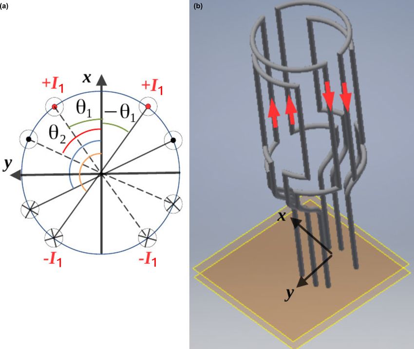
118                                                                                          P. de Pellegars et al.: SHS MRI coils

2   NMR probe overview

At the beginning of NMR history, saddle coil was general-
ized in NMR experiment because of its homogeneity and its
convenience, especially the sample arrangement inside the
coil (Hoult and Richards, 1976). A very important enhance-
ment of RF coil was then proposed by Hayes et al. (1985)
through the birdcage resonator. This resonator takes advan-
tage of the cosine current density distribution, known to pro-
mote magnetic field homogeneity, by means of capacitors
producing a phase shift of the current along the circumfer-
ence. Another type of MRI cosine coil, inspired from older
work (Clarck, 1938), was proposed in Bolinger et al. (1988).
It consisted in approaching the cosine current distribution by
positioning the electrical conductor along the circumference
of a circle following a geometric rule (i.e., an equal distance
of the conductor projection along the diameter circle). It was
recently proposed to enhance the magnetic field homogene-
ity of the Bolinger coil by means of the space harmonics           Figure 1. (a) Electrical conductors of angular positions (θ ), flown
                                                                   by currents In , are distributed along the circumference. (b) Illustra-
suppression (SHS) method (Coillot et al., 2016a). The effi-
                                                                   tion of a saddle-like SHS coil with two pairs of coils.
ciency of the SHS method was demonstrated thanks to nu-
merical finite element method analysis. SHS method was
then extended to enhance the homogeneity of the coils by           3.1   Sensitivity of saddle-like SHS coil
adjusting both the angular position of the wires (distributed
along the circle circumference) and the current magnitude          From Biot–Savart law the magnetic field contribution for the
flowing through the wires (Sidi-Boulenouar et al., 2018).          four wires of the nth coil can be determined. We assume
The extended method efficiency was illustrated through the         that the straight conductors forming the coil have a height
realization of a spherical shape distributed coils creating a      L. They are located at a distance R to the z axis, at an an-
highly homogenous static magnetic field for NMR device.            gular position θn from either side of the x axis and are flown
This work concerns the fabrication of a radio-frequency coils      by a current In . The current flowing through these four wires
for NMR and MRI based on SHS method in axisymmetric                will produce magnetic field contribution (Bwire ) in the y-axis
case for a finite-size geometry.                                   direction, given by Eq. (1). The details of the calculation are
                                                                   reported in Appendix A.
3   Study of saddle-like SHS coil                                                       µ0 In    L
                                                                   Bwiren (0, 0, 0) =         p          cos(θn )                     (1)
                                                                                        π R R 2 + (L/2)2
The SHS coil, as depicted on the left-hand side of Fig. 1,
consists in N pair of coils represented by distributed electri-    Next, the magnetic field contribution (at the coil center) of
cal conductors along z axis. For instance, the nth coil will       the arc portion (Barcn ) in the y-axis direction is given by
consist of four wires located at θn angular positions from ei-     Eq. (2). The details of the calculation are reported in Ap-
ther side of the x axis. Each coil owns Nn conductors flown        pendix A.
by a current in . Thus, the nth coil will be represented by its
ampere-turn number expressed as In = Nn in . The θn angular                                2µ0 RLIn
positions, enhancing the magnetic field coil homogeneity, are      Barcn (0, 0, 0) =                      cos(θn )                    (2)
                                                                                       (R 2 + (L/2)2 )3/2
determined by applying the SHS method. The turns are then
closed by connecting the electrical conductors through arc         Consequently, the total field at the center (BSHS =
                                                                     N (Bwire (0, 0, 0)+Barc (0, 0, 0)) in the y-axis direction)
                                                                   6n=1
portions on the upper and lower parts forming the so-called                   n               n
“saddle-like SHS coil’, as illustrated on the right-hand side      produced by the N pairs of coils of the saddle-like SHS coil
of Fig. 1) for two pairs of coils. In the following, we will fo-   will be
cus on the performance of the saddle-like SHS coils in terms
                                                                                µ0 L         1           2R
of sensitivity and SNR, the homogeneity of SHS coils having        BSHS = p                     + 2
been discussed in previous works.                                            R 2 + (L/2)2 π R R + (L/2)2
                                                                          N
                                                                         6n=1 In cos(θn ).                                            (3)

                                                                   Lastly, by assuming that coils are flown by identical currents
                                                                   (I = In ∀n), the coil sensitivity (Scoil = BSHS /I , cf. Hoult

J. Sens. Sens. Syst., 9, 117–125, 2020                                                     www.j-sens-sens-syst.net/9/117/2020/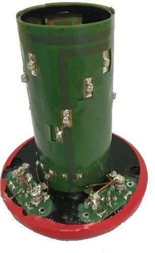
P. de Pellegars et al.: SHS MRI coils                                                                                             119

and Richards, 1976) can be written as                               Table 1. Comparison of coil sensitivities obtained by numerical
                                                                  simulation versus coil sensitivities and SNR deduced from the ana-
             µ0 L        1          2R                              lytic model. The obtained sensitivities and SNR values are normal-
Scoil ∝                     +
          R 2 + (L/2)2 π R R 2 + (L/2)2
        p
                                                                    ized with respect to the SHS2 coil.
       N
      6n=1 cos(θn ).                                         (4)                                         SHS 2   SHS 4   SHS 6
Consequently, the induced voltage (e(t)), using Hoult for-                 relative Scoil (simulated)        1     1.9     2.81
mula, is expressed as                                                      relative Scoil (calculated)       1    1.91     2.81
                ∂δmxy (t)                                                  relative SNR (calculated)         1    1.35     1.63
e(t) = −Scoil             ,                                  (5)
                  ∂t
where δmxy (t) is the magnetic moment in x–y plane and Scoil        Thus, the SNR of the coil is deduced except for a factor, by
is the coil sensitivity factor given by Eq. (4). Since the mag-     combining induced voltage (Eq. 6) and the rms voltage noise
netic moment in x–y plane precesses at Larmor angular fre-          (Eq. 9):
quency ω0 , the induced voltage becomes Eq. (6):
                                                                                   N cos(θ )
                                                                                 6n=1
                                                                          δm               n
|e(j ω0 )| = Scoil ω0 δmxy .                                 (6)    SNR ∝ √ q                      .                              (11)
                                                                           N L + R(π − 26 N θn /N)
                                                                                         n=1
3.2    Signal-to-noise ratio of saddle-like SHS coil
                                                                    The SNR improvement can then be appreciated by compar-
In this section we will focus on the intrinsic SNR of the SHS       ing the SHS4 and SHS6 coils SNR to the one of SHS2 (i.e.,
coil. We assume round wires and a strong skin effect regime         the saddle coil). For this purpose, we will consider the angle
(i.e., skin depth δ much smaller than wire radius); we neglect      values for one, two and three pairs of coils obtained by the
the proximity effect occurring between closed conductors.           SHS method (Coillot et al., 2016a) and reiterated here:
Under these approximations, the equivalent copper section
of the wire is approximated by Swire = 2π rw δ, where rw is             – SHS2 (1 pair): θ1 = 30◦
the conductor wire radius. On the other side the length of the
                                                                        – SHS4 (2 pairs): θ1 = 12◦ and θ2 = 48◦
coil conductor is expressed as Lcoil = 4(L + R × (π − 2θn )).
Thus, the electrical resistance of the nth pair of coils (Resn ),       – SHS6 (3 pairs): θ1 = 11.56◦ , θ2 = 26◦ and θ3 = 56◦ .
forming an angle θn , is written as
                                                                    We assume the height-to-radius ratio known  √ to optimize the
       2ρ(L + R × (π − 2θn ))                                       sensitivity of the saddle coil (i.e., L = 2R 2; see Mispelter
Resn =                        ,                              (7)
              π rw δ                                                et al., 2006). In this case, the normalized SNR value estima-
                                                                    tion (reported in Table 1) shows a significant enhancement
where
√        ρ is the conductor material resistivity and δ =
                                                                    for SHS4 and SHS6 with respect to the conventional SHS2
  2ρ/µω is the skin depth (µ is the magnetic permeability
                                                                    (formal saddle coil).
and ω is the pulsation). Assuming the coils are connected in
series, the total resistance (Res) will be the sum of each pair
of coil resistance. We then deduced from Eq. (7) the total          4     SHS coils prototypes: designs and experimental
resistance equation:                                                      results

       N                2Nρ                    N                    Various SHS coils are customized in our laboratory, at two
Res = 6n=1 Resn =              (L + R × (π − 26n=1 θn /N )). (8)
                        π rw δ                                      extreme frequencies 336 kHz and 128 MHz (corresponding
                                                                    to the 1 H Larmor frequency under respectively 8 mT NMR
   Lastly, by assuming a main noise contribution due to             and 3 T MRI) in order to compare their performances in
Johnson–Nyquist noise (i.e., whose power spectrum density           terms of SNR and magnetic field homogeneity (at least for
is expressed 4kTRes, where k is the Boltzmann constant and          the 3 T MRI case).
T the temperature in K), the rms voltage noise (vn ) of the
coil over a frequency range (BW) is deduced from Wiener–
                                                                    4.1    SHS coils at low magnetic field (8 mT)
Khinchin theorem application (Khintchine, 1934):
      √                                                             In the context of a low magnetic field NMR dedicated to
vn = 4kTRes × BW.                                       (9)         agronomic studies in planta (Sidi-Boulenouar et al., 2018),
                                                                    we have designed two SHS coils, referred to as SHS2 and
The intrinsic signal-to-noise ratio (SNR) is defined as
                                                                    SHS6 (see Fig. 2). The size and geometry of the coils were
         |e(j ω0 )|                                                 imposed by the context of the agronomic study: measure-
SNR =               .                                       (10)    ments on a sorghum stem. That led us to choose a 30 mm
            vn

www.j-sens-sens-syst.net/9/117/2020/                                                       J. Sens. Sens. Syst., 9, 117–125, 2020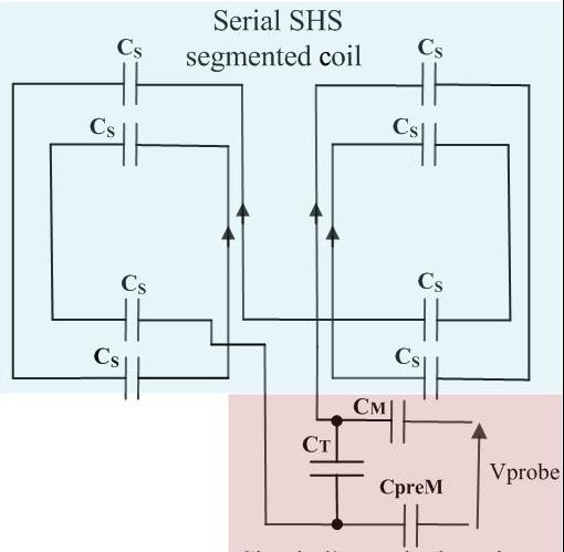
120 P. de Pellegars et al.: SHS MRI coils
Figure 2. SHS clampable coils dedicated to the low-field NMR
.
(8 mT) device. Their resonant frequency was tuned closed to
336 kHz (corresponding to the 1 H Larmor frequency at 8 mT). Figure 3. Electrical circuit of the segmented SHS4 coil (3 T pro-
Right figure represents the SHS2 clampable coil and left figure the totype) with tuning–matching circuit: CS is a fixed segmentation
SHS6. The supporting structure has been realized by 3D printing. capacitance, CT is a variable capacitance, CpreM is a fixed match-
ing capacitance and CM is a variable capacitance allowing to match
finely the impedance of the coil near the Larmor frequency
diameter and 40 mm height coil. For practical reasons we
used 0.5 mm diameter insulated copper wire as a compro-
mise between the need of high diameter wire (to reduce ther- cage probe and SHS coils used at 3 T were fed through a
mal noise) and the mechanical constraints (flexibility for the power splitter device. All the SHS coils were prototyped for
winding feasibility). Lastly, the turn number (120 turns, dis- the purpose of the study within our lab. The same device was
patched in three pairs of coils for SHS6) was chosen to get a used for both coils.
self-resonance frequency of each coil closed to the 1 H Lar-
mor frequency. These coils have the particularity to be clam-
4.2.2 SHS4 coil 3 T prototype
pable in order to manage both the integrity of the plant and
the versatility of the NMR instrument. At higher frequency, MRI probe designer must take care that
The measured quality factor of the SHS2 and SHS6 coils the coil length remains smaller than a fraction of the wave-
were respectively 40 and 80. The SNR of a NMR experiment length (∼ 1/10) at the frequency of interest. When this is not
performed on a same water sample (4 cm3 volume) under the the case, the MRI coil must be segmented (Mispelter et al.,
same pulse condition has exhibited a factor of 3 enhancement 2006) to ensure that the quasi-static magnetic field hypoth-
between the two SHS coils. The details of the testing con- esis is suitable. For the high field condition (i.e., implying
ditions are reported in Sidi-Boulenouar (2018b). This SNR high frequency operating), the coil wire of the SHS coil must
enhancement, in favor of the SHS6 coil, is slightly higher be segmented as illustrated in Fig. 3.
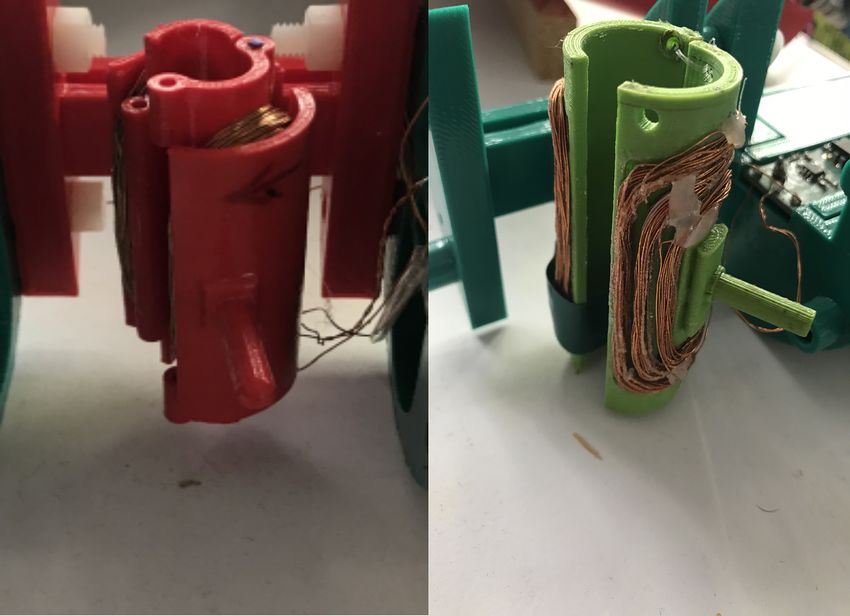
than the expected one (cf. Table 1). This enhancement could Finally, a quadrature-driven SHS4 coil prototype (illus-
be a consequence of the expected homogeneity improvement trated in Fig. 4), dedicated to 1H measuring in a small-
since the quantity of magnetization measurable is related to animal 3 T MRI, has been constructed. Its dimensions were
the RF field homogeneity. chosen identical to the ones of the reference birdcage given
above. The coil itself is realized on a flexible printed circuit
board with a copper ribbon width equal to 3 mm. The flex-
4.2 SHS coils at high magnetic field (3 T) ible circuit includes pads to welcome the segmentation ca-
4.2.1 Experimental setup pacitors. To allow the quadrature driving, two identical flex-
ible circuits were used. Each flexible circuit was associated
A small animal 3 T MRI from RS2 D company was used. The with its own tuning and matching circuit (whose configura-
1 H resonant frequency into this 3 T MRI is 128 MHz. The tion circuit is similar to the one presented in Coillot et al.,
reference MRI probe consists in a quadrature decoupled bird- 2016b). The segmented capacitance values of the prototypes
cage (from MRI Tools company) whose dimensions are as are experimentally determined to coincide with the electrical
follows: coil length = 80 mm and inner diameter = 42 mm. resonance and Larmor frequencies. For the SHS 6 prototype
The outer tube diameter is = 99 mm in order to guide the CS = 44 pF was chosen and the coil was divided into 4 seg-
antenna into the 100 mm diameter tunnel of the MRI. Bird- ments of length ∼ 25 cm in order to equalize with electrical
J. Sens. Sens. Syst., 9, 117–125, 2020 www.j-sens-sens-syst.net/9/117/2020/P. de Pellegars et al.: SHS MRI coils 121
Figure 5. (a) is the one obtained using the quadrature birdcage
while (b) has been obtained using the quadrature SHS4 coil. The
imaging sequence is a MRI spin echo sequence with following pa-
rameters: TE = 10 ms (echo time), TR = 600 ms (repetition time),
field of view = 50 mm × 50 mm, slice thickness = 1 mm, average =
1 and resolution = 256 × 256).
Figure 4. Quadrature SHS4 serial coil dedicated to 1 H 3 T MRI
(80 mm length and 42 mm internal diameter). The coils are realized
on a same flexible printed circuit board including the pads to wel- 5 Discussion
come the segmentation capacitors. Two tuning–matching PCB, for
respectively 0 and 90◦ driving, are inserted on the lower part of the The experimental SNR comparison of SHS prototypes at low
coil. and high magnetic field with respect to both saddle coil and
birdcage coil validated the modeled SNR increase. This SNR
Table 2. SNR comparisons between birdcage coil, saddle coil and increase was also confirmed between SHS4 and birdcage us-
SHS4 measured on the same sample, with identical pulse sequence ing quadrature-driven coil (∼ 35 %). However, it is notice-
parameters, in a 3 T MRI from RS2 D; n/a denotes not applicable. able that the single- and quadrature-channel mode exhibit a
SNR difference higher than the classical 3 dB. We hypothe-
SNR Measured Birdcage SHS2 (saddle) SHS 4 size this difference is attributable to this non-optimal config-
Single channel 566 498 1075 uration. The homogeneity of quadrature SHS4 coil proven by
Quadrature 1050 n/a 1423 image acquiring is roughly comparable to the one of birdcage
(also in quadrature), making the saddle-like SHS coil a rele-
vant MRI probe competitor. However, the superiority of SHS
coil could be limited for higher-volume samples in which
resonance frequency to the Larmor one. CT , CM and CpreM the noise will become dominated by magnetic and dielectric
are respectively the tuning, matching and “pre-matching ca- noise. From Eq. (11) we can roughly express the SNR de-
pacitances. CT and CM are non-magnetic variable capaci- 6 N cos(θ )
pendency as ∝ n=1√ n ; thus, for instance using four pairs
tances from VOLTRONICS, while CS and CpreM are non- N
magnetic fixed capacitances from TEMEX. of coils, the SNR of the SHS coil would increase by approx-
imately a factor of 2. However, the increased of number of
pairs of coils could be limited by complexity and especially
at high frequency where the occurrence of the proximity ef-
4.2.3 A comparison: SHS4 coil versus birdcage
fect becomes preponderant.
Images have been acquired using the 3 T MRI from RS2 D
company using a spin echo sequence. The sample consisted 6 Conclusions
in a cylindrical tube (26 mm diameter – 38 mm length) filled
of water + CuS04 (allowing a decrease in the longitudinal re- The SHS method allows one to easily determine the position
laxation time). The images obtained using a 12-leg quadra- of electrical conductor favoring the production of a homoge-
ture birdcage coil on one hand and quadrature SHS4 coil on nous magnetic field. The method was previously tested in the
the other hand are reported in Fig. 5. Probes were fed through context of spherical coil for static magnetic field. The present
a 0–90◦ hybrid coupler device. For testing in single-channel work concerned the design of NMR or MRI probes based on
mode the hybrid coupler was used through the 0◦ channel, this method. Saddle-like SHS coils have been constructed for
while a 50 was put at the output of the 0◦ channel. different frequency regimes (from 336 kHz up to 128 MHz)
Next, the SNR measurements between different 1 H 3 T in the context of 1 H NMR and MRI. The saddle-like SHS
coils (i.e., birdcage coil, saddle coil and SHS4 coil, single coil has been proved to be driven in quadrature. The exper-
channel or quadrature-driven) are summarized in Table 2. imental comparisons between saddle-like SHS coil, saddle
www.j-sens-sens-syst.net/9/117/2020/ J. Sens. Sens. Syst., 9, 117–125, 2020122 P. de Pellegars et al.: SHS MRI coils coil and commercial birdcage of comparable sizes validate the higher performances in terms of both homogeneity and SNR of the SHS coils. The higher performance obtained makes the SHS probe valuable for NMR and MRI exper- iment. Additionally, the great simplicity of design of SHS coils, with respect to the complexity of the birdcage, should be highlighted. J. Sens. Sens. Syst., 9, 117–125, 2020 www.j-sens-sens-syst.net/9/117/2020/
P. de Pellegars et al.: SHS MRI coils 123
Appendix A: Detailed calculation of Bwiren and which becomes
Barcn 1
cos(arctan(u)) = √ . (A6)
We consider first a single wire “1” of height L parallel to z 1 + u2
and centered in the x–y plane whose middle is located at a By combining these equations we finally get
distance R from the orthonormal, forming an angle θ with x u
sin(arctan(u)) = √ . (A7)
axis, while α corresponds to the angle between the position 1 + u2
vector (r) and the x–y plane. The magnetic field generated
Thanks to the writing of sin(arctan(u)) we express the mag-
by this “1” wire at the center of the SHS coil is expressed
netic field:
using Biot–Savart law:
sin(θ )
µ0 I L
µ0 I dl ∧ r B= cos(θ ) .
dB = , (A1)
p
4π R R 2 + (L/2)2
4π k rk3 0
where dl = [0; 0; dz], √ r = [R cos(θ ); −R sin(θ ); z], Lastly, we sum the contribution of the four wires. By writing
µ0 I √ L
z = R tan α and k r k= R 2 + z2 , which becomes Bw = 4πR 2 2
, each magnetic field contribution for
R +(L/2)
k r k= R/ cos(α). Thus dz is expressed R/cos2 α × dα. wires 1 − 4 is expressed
It results that dB has only components in the x–y plane:
B 1 = Bw [sin(θ ); cos(θ ); 0] (A8)
Rdz sin(θ) B 2 = Bw [− sin(θ); cos(θ ); 0] (A9)
µ0 I
dB = Rdz cos(θ) . B 3 = Bw [− sin(θ); cos(θ ); 0] (A10)
4π k rk3 0
B 4 = Bw [sin(θ ); cos(θ ); 0]. (A11)
Then, Thus the resultant magnetic field of the wires portion for nth
coil (Bwiren ), at an angular position θn and flown by a current
sin(θ)
µ0 I In , will have contribution in y-axis direction which is given
dB = cos(α)dα cos(θ ) .
4π R by
0
µ0 In L
Bwiren = cos(θn ). (A12)
The integration of dB over the wire length (from −L/2 to
p
π R R 2 + (L/2)2
+L/2) is expressed
Next, the contribution of an arc portion (in the x–y plane,
arctan(L/(2R))
Z
sin(θ ) thus z = 0) is obtained by writing the elementary circuit por-
µ0 I tion: dl = [Rdθ cos(θ − π/2); Rdθ sin(θ − π/2); 0] and the
dB = cos(α)dα cos(θ )
4π R 0 distance vector r = [R cos(θ ); R sin(θ ); z]. Since two arc por-
− arctan(L/(2R)) tions are opposite, the opposite elementary circuit portion is
dl 0 = [Rdθ cos(π/2 − θ ); Rdθ sin(π/2 − θ ); 0]. The resulting
sin(θ )
µ0 I
B= sin(arctan(L/(2R))) cos(θ ) . contribution of dl + dl 0 produces a magnetic field contribu-
2π R 0 tion (dB arc1 ) given by
Let us now calculate sin(arctan(u)) where we define θ = −2Rzdθ cos(θ − π/2)
µ0 I 2R 2 dθ sin(θ ) cos(θ − π/2) .
arctan(u). First, we start from tan(θ ) = sin(θ )/ cos(θ ), which dB arc1 = 2
(R + z2 )3/2) 0
can be rewritten
sin(arctan(u)) Then, the same contribution produced by the two opposite
tan(arctan(u)) = , (A2) arc but shifted at z = L/2 becomes
cos(arctan(u))
−2R(z − L/2)dθ cos(θ − π/2)
which becomes 2R 2 dθ sin(θ ) cos(θ − π/2)
dB arc1 = α1
0
sin(arctan(u)) = u × cos(arctan(u)). (A3)
,
Next, since µ0 I
where α1 = (R 2 +(z−L/2) 2 )3/2) . Similarly, the contribution of
the two arcs at position z = −L/2 and flown by current −I
1 + tan2 (θ ) = 1/cos2 (θ ), (A4)
is written as
we get −2R(z + L/2)dθ cos(θ − π/2)
dB arc2 = α2 2R 2 dθ sin(θ ) cos(θ − π/2) ,
1 + tan2 (arctan(u)) = 1/cos2 (arctan(u)), (A5) 0
www.j-sens-sens-syst.net/9/117/2020/ J. Sens. Sens. Syst., 9, 117–125, 2020124 P. de Pellegars et al.: SHS MRI coils
µ0 I
where α2 = − (R 2 +(z+L/2) 2 )3/2) . The combination of dB arc2
and dB arc2 at the center of the coil (z = 0) is written as
2RLdθ cos(θ − π/2)
µ0 I
dB arc = 2 0 .
(R + (L/2)2 )3/2) 0
Lastly, the integration of dB arc over θ will be
2µ0 RLIn
dBarcn = cos(θn ). (A13)
(R 2 + (L/2)2 )3/2
By integration over θn , the total contribution on y axis of the
arc portion at the center of the coil (Barcn ) is given by
2µ0 RLIn
Barcn = cos(θn ). (A14)
(R + (L/2)2 )3/2
2
J. Sens. Sens. Syst., 9, 117–125, 2020 www.j-sens-sens-syst.net/9/117/2020/P. de Pellegars et al.: SHS MRI coils 125
Data availability. All the required data to reproduce the experi- References
ment are given in the body of the paper (geometric parameters of
the MRI coils, the electrical component values, and the parameters Bloch, F.: Nuclear Induction, Phys. Rev., 70, 460–474, 1946.
of the MRI pulse sequence). Bolinger, L., Prammer, M. G., and Leigh, J. S.: A Multiple-
Frequency Coil with a Highly Uniform B1 Field, J. Magn. Re-
son., 81, 162–166, 1988.
Author contributions. PdP was responsible for the high mag- Clark, J. W.: A new method for obtaining a uniform magnetic field,
netic field (9.4 and 3 T) SHS MRI coil design and testing and con- Rev. Sci. Instrum., 9, 320–322, 1938.
tributed to writing the paper. LP carried out the high magnetic field Coillot, C., Nativel, E., Zanca, M., and Goze-Bac, C.: The magnetic
(9.4 and 3 T) SHS MRI coil design and testing. RSB carried out field homogeneity of coils by means of the space harmonics sup-
the low magnetic field (8 mT) SHS coil design and testing and also pression of the current density distribution, J. Sens. Sens. Syst.,
contributed to writing the paper. MZ carried out the SHS conceptu- 5, 401–408, https://doi.org/10.5194/jsss-5-401-2016, 2016a.
alization and modeling. EN carried out the SHS conceptualization Coillot, C., Sidiboulenouar, R., Nativel, E., Zanca, M., Alibert, E.,
and modeling. EA was responsible for the mechanical design of the Cardoso, M., Saintmartin, G., Noristani, H., Lonjon, N., Lecorre,
3 T coils. SR was responsible for the mechanical design of the 8 mT M., Perrin, F., and Goze-Bac, C.: Signal modeling of an MRI rib-
coils. MC managed the high magnetic field MRI tests. JLV, together bon solenoid coil dedicated to spinal cord injury investigations,
with NB, obtained the clampable MRI coil solution for plants, and J. Sens. Sens. Syst., 5, 137–145, https://doi.org/10.5194/jsss-5-
they were responsible of funding and supervision of each of the two 137-2016, 2016b.
projects (grant no. 1504-005 and Pari scientifique INRA). CGB is Hayes, C. E., Edeutein, W. A., Schenck, J. F., Mueller, O. M., and
the head of the MRI facility at Montpellier University. JM managed Eash, M.: An Efficient Highly Homogeneous Radiofrequency
3 T MRI testing and comparisons. RS is the head of the 3 T MRI Coil for Whole-Body NMR Imaging at 1.5T, J. Magn. Reson.,
facility at RS2 D. CC carried out the SHS conceptualization, model- 63, 622–628, 1985.
ing, MRI coil tests, and manuscript writing, reviewing, and editing. Hoult, D. I. and Richards, R. E.: The signal-to-noise ratio of the nu-
clear magnetic resonance experiment, J. Magn. Reson., 24, 71–
85, 1976.
Khintchine, A.: Math. Ann., 109, 604–615,
Competing interests. The authors declare that they have no con-
https://doi.org/10.1007/BF01449156, 1934.
flict of interest.
Mispelter, J., Lupu, M., and Briguet, A.: NMR probehads for bio-
physical and biomedical experiments: theoretical principles and
practical guidelines, Imperial College Press, 2006.
Acknowledgements. The authors would like to thank SATT
Sidi-Boulenouar, R.: Dynamic monitoring of water status of
AxLR (who funded the prototyping program), CNRS (who funded plants in the fields under environmental stress: Design of a
in 2018 the so-called “Défi instrumentation aux limites”), Agropolis portable NMR and applied to sorghum, Physics [physics], Uni-
fondation in the context of APLIM (Advanced Plant Life Imaging) versité Montpellier, available at: https://tel.archives-ouvertes.fr/
project (contract 1504-005) and Pari scientifique INRA département tel-02139254/document (last access: 17 March 2020), 2018.
Environnement et Agronomie. Sidi-Boulenouar, R., Reis, A., Nativel, E., Buy, S., de Pellegars,
P., Liu, P., Zanca, M., Goze-Bac, C., Barbat, J., Alibert, E.,
Verdeil, J.-L., Gatineau, F., Bertin, N., Anand, A., and Coillot,
Financial support. This research has been supported by the C.: Homogenous static magnetic field coils dedicated to portable
SATT AxLR, the Centre National de la Recherche Scientifique nuclear magnetic resonance for agronomic studies, J. Sens.
(Défi Instrumentation aux Limites), the Agropolis Fondation (grant Sens. Syst., 7, 227–234, https://doi.org/10.5194/jsss-7-227-2018,
no. 1504-005), and the INRA (Pari scientifique INRA département 2018.
Environnement et Agronomie).
Review statement. This paper was edited by Marco Jose da Silva
and reviewed by two anonymous referees.
www.j-sens-sens-syst.net/9/117/2020/ J. Sens. Sens. Syst., 9, 117–125, 2020You can also read