How does access to this work benefit you? Let us know!
←
→
Page content transcription
If your browser does not render page correctly, please read the page content below
City University of New York (CUNY)
CUNY Academic Works

Publications and Research                                               New York City College of Technology

2021

Discovering Kepler’s Third Law from Planetary Data
Boyan Kostadinov
CUNY New York City College of Technology

Satyanand Singh
City University of New York, Graduate Center

How does access to this work benefit you? Let us know!
More information about this work at: https://academicworks.cuny.edu/ny_pubs/751
Discover additional works at: https://academicworks.cuny.edu

This work is made publicly available by the City University of New York (CUNY).
Contact: AcademicWorks@cuny.edu
Discovering Kepler’s Third Law from Planetary Data
                                     ICTCM 2020 Conference Proceedings

                                 Boyan Kostadinov∗                 Satyanand Singh†

                                New York City College of Technology, CUNY

                                                        Abstract
           In this data-inspired project, we illustrate how Kepler’s Third Law of Planetary Motion can be
       discovered from fitting a power model to real planetary data obtained from NASA, using regression
       modeling. The power model can be linearized, thus we can use linear regression to fit the model parameters
       to the data, but we also show how a non-linear regression can be implemented, using the R programming
       language. Our work also illustrates how the linear least squares used for fitting the power model can
       be implemented in Desmos, which could serve as the computational foundation for this project at a
       lower course level. This paper is based on our ICTCM 2020 talk with the same title. We included two
       NASA inspired student projects at the calculus level that were developed with the support of the Opening
       Gateways grant at New York City College of Technology.

Contents
1 Introduction                                                                                                                                                     1

2 Discovering Kepler’s third law from planetary                 data                                                                                               2
  2.1 Kepler’s law of harmonies . . . . . . . . . . . .         . . . .   .   .   .   .   .   .   .   .   .   .   .   .   .   .   .   .   .   .   .   .   .   .    2
  2.2 Kepler’s third law from least squares . . . . . .         . . . .   .   .   .   .   .   .   .   .   .   .   .   .   .   .   .   .   .   .   .   .   .   .    3
  2.3 Visualizing the planetary data . . . . . . . . . .        . . . .   .   .   .   .   .   .   .   .   .   .   .   .   .   .   .   .   .   .   .   .   .   .    3
  2.4 Fitting the model with linear least squares . . .         . . . .   .   .   .   .   .   .   .   .   .   .   .   .   .   .   .   .   .   .   .   .   .   .    4
  2.5 Fitting a linear model without an intercept . .           . . . .   .   .   .   .   .   .   .   .   .   .   .   .   .   .   .   .   .   .   .   .   .   .    5
  2.6 Kepler’s third law rediscovered . . . . . . . . .         . . . .   .   .   .   .   .   .   .   .   .   .   .   .   .   .   .   .   .   .   .   .   .   .    5
  2.7 Fitting the model with nonlinear least squares .          . . . .   .   .   .   .   .   .   .   .   .   .   .   .   .   .   .   .   .   .   .   .   .   .    6
  2.8 Using regression in Desmos . . . . . . . . . . .          . . . .   .   .   .   .   .   .   .   .   .   .   .   .   .   .   .   .   .   .   .   .   .   .    6

3 NASA inspired STEM applications at the calculus level                                                                                                           8
  3.1 Modeling a rocket’s path by using a differential equation . . . . . . . . . . . . . . . . . . . . .                                                         8
  3.2 Star encounters in the Milky Way . . . . . . . . . . . . . . . . . . . . . . . . . . . . . . . . . .                                                        8

4 Ackowledgements                                                                                                                                                 10

5 Appendix: Installing R and RStudio                                                                                                                              11

1      Introduction
In this data-inspired project, we illustrate how Kepler’s Third Law of Planetary Motion can be
discovered using regression modeling to fit a power model to real planetary data obtained from NASA.
    ∗ Mathematics   Department, bkostadinov@citytech.cuny.edu
    † Mathematics   Department, ssingh@citytech.cuny.edu

                                                            1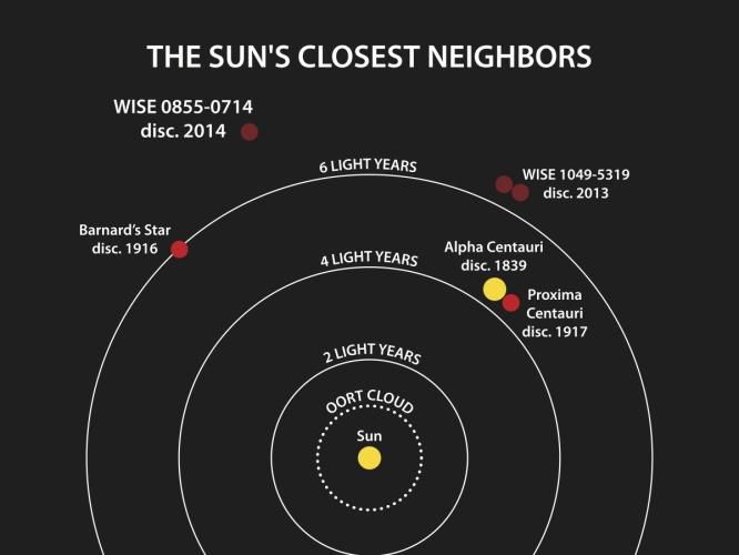
The power model can be linearized, thus we can use linear regression to fit the model parameters to the data,
but we also show how a non-linear regression can be implemented using the R programming language.
In the second part of the paper, we discuss how the linear least squares used for fitting the power model can
be implemented in Desmos, which could serve as the computational foundation for this project at a lower
course level that does not require programming with a high-level programming language such as R or Python.
For the R implementations, we use R Markdown notebooks in RStudio, [1, 2]. RStudio can also be accessed
in the RStudio Cloud [3]. A very short introduction to R can be found in [4]. We use the tidyverse, broom,
knitr and modelr R packages.
For additional references on using R in undergraduate mathematics courses, we refer the reader to the papers
[11, 12, 13, 14].

2     Discovering Kepler’s third law from planetary data
2.1     Kepler’s law of harmonies
Kepler’s third law is an elegant example of a power law between the period of an orbiting body and its
average distance to the object it orbits. Even comets such as Halley’s comet, shown below, obeys Kepler’s
law and from its period one can calculate the average distance of Halley’s comet from the Sun.

                                Figure 1: Halley’s comet flying through space.

    • Kepler’s laws can be derived from Newton’s laws of motion and his law of gravity.
    • Kepler’s laws allow us to use them as tools to do space explorations and make predictions.
    • Kepler’s third law allows us to find the most efficient trajectory from Earth to Mars, which is called the
      Hohmann transfer orbit. Kepler’s third law implies that this orbit has to be an ellipse that touches
      both orbits and has the shortest possible semimajor axis.
Newton’s generalization of Kepler’s third law takes the form:

                                                       4π 2
                                             P2 =               a3 ,                                        (1)
                                                    G(M1 + M2 )

where P is the period of the orbit, a is the semi-major axis of the orbit, M1 is the mass of the first body and
M2 is the mass of the second body, and G is the gravitational constant.
For planets orbiting the sun, Msun is much bigger than the mass of any planet Mplanet , and Msun + Mplanet ≈
Msun , thus we obtain Kepler’s version of the law:

                                                        2
Table 1: NASA’s Normalized Planetary Data
Distance D [AU] Period T [Earth’s Years] ln(D) ln(T)
Mercury 0.3870321 0.2409639 -0.9492477 -1.4231083
Venus 0.7232620 0.6152793 -0.3239837 -0.4856790
Earth 1.0000000 1.0000000 0.0000000 0.0000000
Mars 1.5233957 1.8811610 0.4209419 0.6318891
Jupiter 5.2045455 11.8592552 1.6495324 2.4731086
Saturn 9.5822193 29.4277108 2.2599092 3.3819368
Uranus 19.2012032 83.7595838 2.9549729 4.4279506
Neptune 30.0474599 163.7458927 3.4027781 5.0983158
Pluto 39.4812834 247.9737130 3.6758267 5.5133227
4π 2
P 2 ≈ Ka3 , K= (2)
GMsun
2.2 Kepler’s third law from least squares
We use planetary data collected from NASA’s Lunar and Planetary Science Division, [5]. The planetary
data in Table 1 were derived from the original NASA data by doing data transformations that consists of
normalizing the distances and the orbital periods in Earth’s units (1AU = 1.496 × 10⁸ km).
We use the normalized planetary data to find a relationship between the average distance from the Sun, given
in AU, and the orbital period, given in Earth’s years. For the model function, we use a power model with
two parameters α and β:
T = αDβ , (3)
where T is the orbital period in Earth’s years and D is the average distance from the Sun in AU. We hope
that this power model will reveal Kepler’s law (2), after we fit it to planetary data.
The R code below creates a dataframe with the normalized planetary data and prints Table 1.
planetTable 2: The linear model fitted to planetary data.
term estimate std.error statistic p.value
(Intercept) -0.0002937 0.0011731 -0.2503724 0.8094889
log(D) 1.4987995 0.0005377 2787.3365339 0.0000000
geom_point(mapping=aes(x=D,y=T,text=planet),data=dataDT,col="red",size=1.5,alpha=0.6) +
labs(x ="Distance D [AU]", y = "Orbital Period T [years]")
250
200
Orbital Period T [years]
150
100
50
0
0 10 20 30 40
Distance D [AU]
Figure 2: The normalized planetary data.
2.4 Fitting the model with linear least squares
We can linearize the power model (3) and then apply linear least squares to fit the model parameters. The
linearization consists of taking the logarithm on both sides:
ln(T ) = ln(α) + β ln(D) (4)
Now, we have a linear model with respect to the unknown parameters γ = ln(α) and β. The response variable
is now y = ln(T ), and the predictor is x = ln(D). Thus, the linearized model can be written as:
y = γ + βx (5)
A single predictor linear model has the R formula y~x, which implements the linear model y = γ + βx. The
R code below fits the model parameters γ and β, and generates Table 2:
model% tidy() %>% knitr::kable(caption="The linear model fitted to planetary data.")
Note that log() is the natural logarithm in R.
4Table 3: The updated linear model fitted to planetary data.
term estimate std.error statistic p.value
log(D) 1.49871 0.0003766 3980.082 0
2.5 Fitting a linear model without an intercept
The intercept (the constant term γ) is not statistically significant since its p-value is about 81%. Thus, we
can update our linear model to one with γ = 0 (α = 1):
y = βx ⇐⇒ T = Dβ (6)
The R code below fits the single model parameter β, and generates Table 3:
model% tidy() %>% kable(caption="The updated linear model fitted to planetary data.")
2.6 Kepler’s third law rediscovered
Thus, we can conclude that β is very likely to be 1.5 in a physical model of our planetary system. Dimensional
analysis would also confirm the value of 1.5. The fitted model then becomes:
T = D3/2 ⇐⇒ T 2 = D3 (7)
This is what Kepler discovered in 1619 with his Third Law, about 400 years ago.
With the right data, we can discover even laws of physics!
In Figure 3, we show the fitted power model T = D3/2 (in blue), and planetary data as red dots.
250
200
Orbital Period T [years]
150
100
50
0
0 10 20 30 40
Distance D [AU]
Figure 3: The fitted power model T = D3/2 (in blue) and planetary data (in red).
5Table 4: The nonlinear least squares fit to planetary data.
term estimate std.error statistic p.value
beta 1.499386 0.0002648 5662.806 0
2.7 Fitting the model with nonlinear least squares
The ability to implement a nonlinear regression is often required for real-world applications, given that models
are often complex and nonlinear, and they cannot be usually linearized. The last part of the lesson is to use
a nonlinear regression to fit the parameters of the planetary model. We use R’s nonlinear regression function
nls() and work with the power model T = αDβ .
For Earth, we have T = D = 1, which implies α = 1, so we can update the physical model to have α = 1,
thus implying again a power model of the form:
T = Dβ (8)
The R code below fits the single model parameter β using non-linear regression, and generates Table 4:
model % tidy() %>% kable(caption="The nonlinear least squares fit to planetary data.")
2.8 Using regression in Desmos
Next, we demonstrate how we can implement a linear or non-linear regression using Desmos, [9], which
can be used even at the calculus level.
You can copy data (with variables as headers) from a spreadsheet and paste it into a blank expression in the
Desmos calculator. Then, you can enter your regression model, for example a linear model:
y1 ∼ ax1 + b (9)
or an exponential model:
y1 ∼ aebx1 (10)
where the parameters a and b will be fitted to the data.
Desmos has a shallow learning curve and we will first generate the linear model. We begin by copying and
pasting the two columns from Table 1 with headings ln T and ln D into the Desmos graphing calculator. In
the Desmos screenshot, x1 and y1 denote ln D and ln T , respectively. Then, move the cursor below the data
to the second blank space and type in the formula for linear regression y1 ∼ ax1 + b. Desmos then computes
and prints the values of the parameters fitted to the data, namely a = 1.4988, b = −0.000293698. Given that
the data come from a physics law, it is not surprising that the goodness of fit of this model is 1 (r2 = 1),
indicating that the regression predictions perfectly fit the data. See Figure 4.
We will now proceed to generate the exponential model. We will mimic the first step outlined above by
pasting the two columns from Table 1 with headers D and T . By default, Desmos labels the headings as x1
and y1 . We relabel the headings in Desmos by D and T , which correspond to the data in Table 1. In the
second blank space we now enter the exponential model T ∼ Dn and Desmos fits the parameter n = 1.49939
to the given data, using regression. See Figure 5.
We suggest that you explore the Desmos animation of Kepler’s Law, found here [10].
6! Untitled Graph Log In or Sign Up " # $
( ) 3 * + .
1
- (
x1 % y1
/
−0.9492476 −1.4231081
−0.3239837 −0.4856790 0
0.0000000 0.0000000
0.4209419 0.6318891
1.6495324 2.4731086
2.2599092 3.3819368
2.9549729 4.4279506
3.4027781 5.0983158
3.6758267 5.5133227
,
2
-
& y1 ~ ax1 + b
STATISTICS RESIDUALS
r2 = 1 e1 plot
r=1
PARAMETERS
a = 1.4988 b = -0.000293698
3
-
4
'
powered by
12
Figure 4: Fitting a linear model in Desmos.
! Untitled Graph Log In or Sign Up " # $
) * 3 + , .
1
- )
D % T
/
0.3870321 0.2409639
0.723262 0.6152793 0
1 1
1.5233957 1.881161
5.2045455 11.8592552
9.5822193 29.4277108
19.2012032 83.7595838
30.0474599 163.7458927
39.4812834 247.973713
2
-
' T ~ Dn
& Log Mode #
STATISTICS RESIDUALS
R2 = 1 e1 plot
PARAMETERS #
n = 1.49939
3
(
powered by
12
Figure 5: Fitting an exponential model in Desmos.
73 NASA inspired STEM applications at the calculus level
3.1 Modeling a rocket’s path by using a differential equation
In May, 2020 SpaceX [6] launched a rocket. For a rocket launched vertically, we can study the rocket’s
velocity as a function of its distance traveled by using Newton’s law of universal gravitation and his second
dv gR2
law of motion. It can be shown that the differential equation v dx = − (x+R) 2 is true, where v is the velocity
of the rocket, R is the radius of the earth and x is the rocket’s distance from the surface of the earth. We are
assuming friction is negligible and that the earth is a spherical object. The mean radius R of the earth is
6371 km. according to NASA [7] and the acceleration due to gravity, g = 9.875 m/s2 .
Figure 6: A rocket liftoff.
2
dv gR
1. Solve the equation v dx = − (x+R) 2 , with the initial condition v(0) = v0 .
r
1
2. Use your solution from problem 1, to show that v = 2gR2 R+x − R1 + v02 .
3. Plot the graph of v(x) verses x, when the initial velocity, v0 = 700 m/s and find the value of x if it
exists when v(x) = 0. Repeat this for v0 = 12500 m/s.
4. By trial and error predict the smallest positive initial velocity v0 such that v(x) will eventually achieve
0 as x increases. Give a practical interpretation of this cut off value of v0 .
5. Answer the following questions:
• 5a When the rocket reaches the top of its trajectory x = L, find its initial velocity, v0 ? Hint: Use
the formula you derived in problem 2 and consider the value of the final velocity v at this instant.
• 5b Use the expression you obtained in part (a) for the velocity which we will now call vL and
compute the limit, ve = limL→+∞ vL .
• 5c Compute the numerical value of ve .
• 5d Give a physical interpretation of ve and compare its value with the value of v0 obtained in
problem 4.
• 5e How does your calculated value for ve , the escape velocity compare with the actual value stated
by NASA? See [8].
6. Further Explorations: Find the escape velocity of the moon and other planets. Compare the values
to Earth’s value and briefly explain how this helps with space explorations.
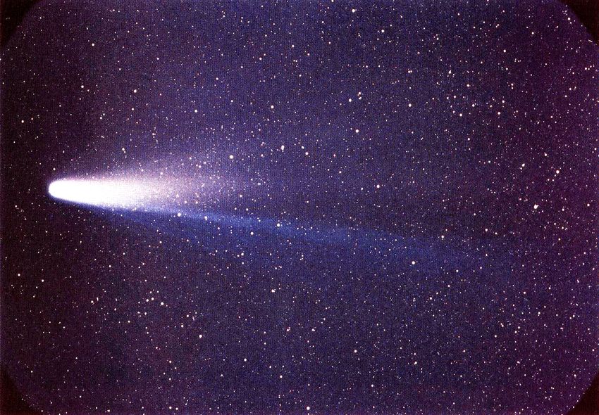
3.2 Star encounters in the Milky Way
3.2.1 Introduction
Stars travel along complex orbits through our galaxy the Milky Way, which is shown in Figure 7.
Here are some curious facts about the Milky Way:
8Figure 7: The Milky Way, and the Sun in the Orion arm of the galaxy.
• Radius: around 50,000 light years, so it is about 100,000 light years across.
• Age: around 14 billion years.
• Stars: 250 billion ± 150 billion.
• Sun’s Galactic rotation period: 240 million years.
• Sun’s distance to Galactic Center: 26,400 ± 1000 light years.
Be careful, light years are not units of time. Look up the definition of light years.
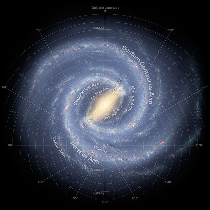
Barnard’s Star is one of the stars closest to the Sun, as shown in Figure 8.
Figure 8: The Sun’s closest neighbors among the stars.
3.2.2 Barnard’s Star trajectory, relative to the Sun
In a Cartesian grid centered at the Sun, the current position of Barnard’s Star can be represented
(approximately) as the point (2.0, 5.67), in units of light years, see Figure 9.
Barnard’s Star travels across the sky so quickly that it traverses the diameter of the full moon every 180
years. In the coordinate system centered at the Sun, the parametric equations for the x and y coordinates of
Barnard’s Star as a function of time can be approximated as follows:
9Figure 9: Barnard’s Star, relative to the Sun.
x(t) = 2 + 0.09t (11)
y(t) = 5.67 − 0.25t, (12)
where t is in thousands of years from the present time, and x and y distance units are in light years. At
time t = 0, (x(0), y(0)) = (2, 5.67) is the current position of Barnard’s Star at the present time.
Answer the following questions:
1. What is the distance from the Sun to Barnard’s Star at the present time?
2. What is the equation of the line y = b + ax that represents Barnard’s trajectory, given by the
parametric equations?
3. Plot the graph of the line obtained in problem 2 first by hand and then using Desmos.
4. At what time, t0 will Barnard’s Star be at its closest to the Sun along its trajectory?
5. Find the minimum distance between the Sun and Barnard’s Star by using:
• 5a A calculus approach based on optimization with derivatives.
• 5b An analytic geometry approach based on vectors or an intuitive geometric argument.
6. Further Explorations: A spaceship leaves the Solar System now in an attempt to reach Barnard’s
Star. Find the velocity vector and its magnitude, i.e. the speed, of this spaceship and the time it will
take to reach Barnard’s Star on its current trajectory, assuming that both the star and the spaceship
travel with constant velocity. Note that given the scale, we can identify the Sun with the Solar System.
4 Ackowledgements
We would like to extend our gratitude to the reviewers for accepting our work and to the Pearson team for
facilitating our presentation. We would like to particularly thank Brooke-Lynn Killingbeck and Lauren
Lopez for their assistance during ICTCM 2020 and for the opportunity to submit this paper to the ICTCM
2020 conference proceedings.
We would also like to thank the project team of Opening Gateways (OG) to Completion: Open
Digital Pedagogies for Student Success in STEM for their support with the development of the NASA
inspired STEM projects, while we were OG Fellows in 2019-2020 at NYC College of Technology, CUNY.
105 Appendix: Installing R and RStudio
We used R Markdown notebooks in RStudio for all computations and visualizations with R. In order to
create PDF output from R Markdown notebooks in RStudio, we need to install either a full TEX distribution
(MiKTeX or MacTeX), or the tinytex R package, in addition to R and RStudio. The following software
installers are available for Windows, Mac, and Linux:
• MiKTeX installers for Windows and Mac: http://miktex.org/download
• MacTeX installer for Mac: http://tug.org/mactex/
• R installers, [1]: http://cran.stat.ucla.edu/
• RStudio installers, [2]: https://www.rstudio.com/
A cloud-based option (free and paid) for computing with RStudio is provided by the R Studio Cloud, [3].
References
[1] The R Project for Statistical Computing. R version 4.0.4 (02-15-2021). http://www.r-project.org. Accessed
March 31, 2021.
[2] RStudio version 1.4.1106. http://www.rstudio.com. Accessed March 31, 2021.
[3] RStudio Cloud. https://rstudio.cloud. Accessed March 31, 2021.
[4] A (Very) Short Introduction to R. http://cran.r-project.org/doc/contrib/Torfs+Brauer-Short-R-Intro.pdf.
Accessed March 31, 2021.
[5] NASA planetary data. https://nssdc.gsfc.nasa.gov/planetary/factsheet/. Accessed March 31, 2021.
[6] SpaceX rocket launches. https://www.spacex.com/launches/. Accessed April 1, 2021.
[7] Earth’s facts. https://nssdc.gsfc.nasa.gov/planetary/factsheet/earthfact.html. Accessed April 1, 2021.
[8] Escape velocity facts. https://www.nasa.gov/audience/foreducators/k-4/features/F_Escape_Velocity.ht
ml. Accessed April 1, 2021.
[9] Desmos calculator. https://www.desmos.com/calculator. Accessed April 1, 2021.
[10] Kepler’s 3rd law in Desmos. https://www.desmos.com/calculator/xskc85kx3c. Accessed April 1, 2021.
[11] Boyan Kostadinov, Johann Thiel and Satyanand Singh (2019), Creating Dynamic Documents with R
and Python as a Computational and Visualization Tool for Teaching Differential Equations, PRIMUS,
29:6, 584-605. DOI: 10.1080/10511970.2018.1472161
[12] Benakli, N., Kostadinov, B., Satyanarayana, A. and S. Singh (2016), Introducing computational thinking
through hands-on projects using R with applications to calculus, probability and data analysis, Int. J.
Mathematics Education in Science and Technology, 48(3): 393–427. DOI: 10.1080/0020739X.2016.1254296
[13] Kostadinov, B. (2013), Simulation insights using R, PRIMUS, 23(3): 208–223.
DOI: 10.1080/10511970.2012.718729
[14] Kostadinov, B. (2018), Predicting the Next US President by Simulating the Electoral College, Journal of
Humanistic Mathematics, 8(1): 64–93. DOI: 10.5642/jhummath.201801.05. Available at: http://scholars
hip.claremont.edu/jhm/vol8/iss1/5
11You can also read