Identifying the density of grassland fire points with kernel density estimation based on spatial distribution characteristics
←
→
Page content transcription
If your browser does not render page correctly, please read the page content below
Open Geosciences 2021; 13: 796–806
Research Article
Zhen Shuo, Zhang Jingyu, Zhang Zhengxiang*, and Zhao Jianjun
Identifying the density of grassland fire points
with kernel density estimation based on spatial
distribution characteristics
https://doi.org/10.1515/geo-2020-0265 or inaccurate point variable, considering the spatial dis-
received September 15, 2020; accepted May 19, 2021 tribution characteristics.
Abstract: Understanding the risk of grassland fire occur- Keywords: grassland fire, risk, spatial cluster, Ripley’s K
rence associated with historical fire point events is critical
for implementing effective management of grasslands.
This may require a model to convert the fire point records
into continuous spatial distribution data. Kernel density 1 Introduction
estimation (KDE) can be used to represent the spatial
distribution of grassland fire occurrences and decrease Grassland fires are considered to be one of the major
the influences historical records in point format with disturbances affecting natural ecosystems in grass-domi-
inaccurate positions. The bandwidth is the most impor- nated regions with human activities, and the emissions of
tant parameter because it dominates the amount of varia- greenhouse gas is a main factor that influences the global
tion in the estimation of KDE. In this study, the spatial climate change [1–4]. Annual fires are also problematic
distribution characteristic of the points was considered to for soil erosion, grass resources, and biodiversity and
determine the bandwidth of KDE with the Ripley’s K func- diminish the production of agriculture and livestock [5].
tion method. With high, medium, and low concentration In this sense, identifying and assessing the risk of grass-
scenes of grassland fire points, kernel density surfaces land fire ignition occurrence are key issues for the ade-
were produced by using the kernel function with four quate design and decision-making of fire management
bandwidth parameter selection methods. For acquiring [6,7].
the best maps, the estimated density surfaces were com- In wildland fire studies, the spatial pattern and distri-
pared by mean integrated squared error methods. The bution of fire events are essential to wildfire managers or
results show that Ripley’s K function method is the best scientists [1]. And continuous distribution surface of fire
bandwidth selection method for mapping and analyzing occurrence is widely used in the explanation for the spatial
the risk of grassland fire occurrence with the dependent pattern of fire risk or the analysis of the influencing factors
by decreasing the inaccuracies and substantial errors of
fire history record as a point with x- and y-coordinates
[1,8,9]. The methods that can convert the fire record point
* Corresponding author: Zhang Zhengxiang, Key Laboratory of into continuous density are needed [8,10].
Geographical Processes and Ecological Security in Changbai Kernel density estimate (KDE) is a nonparametric esti-
Mountains, Ministry of Education, School of Geographical Sciences, mation of deriving a continuous surface with the under-
Northeast Normal University, Changchun 130024, China, lying unknown density function [11]. And it was applied
e-mail: zhangzx040@nenu.edu.cn
to effectively convert point-based events into grid-based
Zhen Shuo: Key Laboratory of Geographical Processes and
Ecological Security in Changbai Mountains, Ministry of Education, distribution for analyses in various disciplines, such as
School of Geographical Sciences, Northeast Normal University, animal home range estimation in wildlife ecology, traffic
Changchun 130024, China accident density estimation, analysis of central business
Zhang Jingyu: Faculty of Geographical Sciences, Beijing Normal districts, and seismic risk analysis in geology [12–14].
University, Beijing 100857, China
In wild fire studies, KDE is used extensively to convert
Zhao Jianjun: Key Laboratory of Geographical Processes and
Ecological Security in Changbai Mountains, Ministry of Education,
fire historic point records into continuous fire occurrence
School of Geographical Sciences, Northeast Normal University, density surfaces for defining the spatial distribution of
Changchun 130024, China, e-mail: Zhaojj662@nenu.edu.cn fire ignition at different scales, analyzing its extent and
Open Access. © 2021 Zhen Shuo et al., published by De Gruyter. This work is licensed under the Creative Commons Attribution 4.0
International License.Density of grassland fire points with KDE 797
distribution, or representing the fire risk associated with The first method does not consider the number of
the influencing factors [6,8,10,15–17]. KDE method has observed points except the polygon of the study area.
also been used in grassland fire analysis [10,17]. The last two methods consider the number of observed
The kernel density function was defined [18] as follows: points and the size of the study area. And these band-
n widths are used to calculate the concentrations of observed
fˆ (x ) =
1
nh2
∑K
i=1
{ s − si
h }, (1) events in a specified area. With a high concentration of
observed events, the value of bandwidth is small. And
n is the total number of observed events, K is the kernel when the concentration is low, the value of bandwidths is
function, h is the bandwidth that defines the searching big [21].
radius of the kernel function, s is the position where the In our previous works, RDmean is used to determine
estimation density value is being calculated, and si is the the bandwidth of the KDE method for providing the
position of each observed event. grassland fire regime studies by the fire density maps
The bandwidth controls the smoothness of the KDE with MODIS fire active production in the eastern Inner
surface, and it is considered more critical than the selec- Mongolia of China [10,17]. Although the results have
tion of kernel functions [19]. A large value of h will pro- appropriately expressed the characteristic of grassland
duce a smooth distribution, but it may cause a loss of fire distribution in the whole study area, when analyzing
details on the resulting surfaces. In contrast, when using the fire occurrence risk in the local area, the calculated
a narrow h, the estimated surface tends to show too many fire density varies markedly with the same influence fac-
finer variations that often obscure the clustering charac- tors. At or near the observed fire points, the density is
teristic [6]. higher. Around the points, the density is lower. Hence,
Some methods were applied to set appropriate band- the risk in the area with the observed points will be over-
widths that are widely used in many studies [20,21]. In estimated and the risk in the area without or near the
one approach, the bandwidth is defined by the mean observed points will be underestimated. These band-
polygon size in the study area [20]. The mean polygon width selection methods don’t consider the spatial corre-
size is computed, and a theoretical square is created that lation of locations of the observed points. Mostly, the
has the same area as the mean polygon. Hence, the band- characteristic of the point distribution pattern was not
width of the square can be defined as the radius of the considered in these methods for defining the bandwidth.
circle around the square, which also is half of the diag- In a specified area with the same number of points, the
onal of the square as follows: characteristic of the distribution can be clustered, random
or disperse, but the concentration characteristic of points in
D
h= , (2) the area can be the same or similar if don’t consider the
2
spatial distribution of events, as shown in Figure S1. Then,
where D is the diagonal of the theoretical square. only using the area and the number of points in the methods
RDmean approach is given based on the calculation of can’t express the characteristic of spatial distribution. In
local mean random distance [20]: the field, once a location is targeted by a fire, nearby loca-
tions face an elevated risk of experiencing the same event
1 A
RDmean = , (3) shortly. Thus, spatial point pattern analysis has been inten-
2 N
sively investigated to reveal the scale, extent, and dynamics
where A is the mean size polygon and N is the average of point events and to test potential patterns related to spa-
number of point events in a polygon. The final value of tial mechanisms of fire occurrence. Due to the distribution
bandwidth is given by multiplying RDmean by two [8]. of wildland fire events is a cluster, the characteristic of the
Another bandwidth based on all of the observed spatial distribution pattern should be considered when
points is defined [22]. Because it does not consider the defining the bandwidth of KDE [24].
area, the value of the bandwidth was altered according to The main purpose of this study is to identify the spatial
the dimension of the area through multiplying it by the continuous distribution surface of grassland fire occur-
square root of the area, and it is named as Willamson rence with improving the bandwidth selection method of
function [23]: KDE by considering the spatial distribution patterns of
(4) observed point events and to provide guidance on which
h = 0.68N−0.2 A ,
method most accurately determines the underlying density.
where N is the number of all observed points, 0.68 is a The study area is in eastern Inner Mongolia, China, which
constant, and A is the study area size. has suffered from a high grassland fire incident rate, using798 Zhen Shuo et al.
KDE methods with MODIS fire active products (for the are dominated by Stipa baicalensis, Filifolium sibiricum,
period from 2001 to 2014). This method demonstrates that and Leymus chinensis. The elevation ranges from 200 to
such a technique, which considers the spatial distribution 1500 m. The Greater Khingan Mountains is located in the
characteristics, can be extended to different spatial data middle region, stretching from the center of the region
analyses. To achieve this objective, several methods of toward the east and west. The elevation gradually decreases,
choosing the bandwidth were applied. Then, the KDE and the topography gradually becomes flatter. The activities
maps were compared to reveal the effects of different band- of the inhabitants lead to accidental fires. Approximately
widths. A case study is expressed by figuring out the dis- 600 wild fires occur annually in this region. In previous
tribution pattern of the spatial point data, and the suitable studies, KDE method was used to access the risk of grassland
bandwidth selection can easily be implemented for geogra- fire in this area, which is why it was chosen as the study area
phical areas. The results of the current research can also be to analyze the bandwidth selection method [10,17].
a valuable reference for policy-making in fire management. In the study area, the MODIS Active Fire Data contain
daily fire pixel coordinate positions and they are most
suitable to determine the spatial and temporal distribu-
tions of fire points. The MODIS Terra and Aqua daily
2 Study area and methods active fire product data are available (MOD14A1 and
MYD14A1). The fire product data set from 2001 to 2014
was downloaded from the Land Processes Distributed
2.1 Study area and data
Active Archive Centre (LP-DAAC) using a web-based
interface known as Reverb, which is a replacement for
Hulunbuir is located in the northeast Inner Mongolia the Warehouse Inventory Search Tool (http://reverb.cs.
Autonomous Region of China, from 47.08°N to 53.23°N washington.edu/). The resolution of the fire product is
and 115.22°E to 126.06°E (Figure 1). The study area is 1 km pixels, in which burning was detected at the times
approximately 681 km long and 703 km wide, covering a of Terra and Aqua satellite overpass under the condition
total area of 252,948 km2. The climate in the region is a of less cloudiness. Calculated from 4 and 11 µm channels,
typical temperate continental monsoon climate, with low, the brightness temperature of fire pixels was obtained
irregular rainfall and extreme temperature variations in based on an algorithm that enhances the detection sen-
summer and winter. The annual mean air temperature sitivity of smaller, cooler fires and decreases the emer-
and precipitation are about −2.3°C and 320 mm, respec- gence of false alerts [25–28].
tively. The vegetation in the eastern Inner Mongolia grass- As the major component of the MODIS active fire
land region consists of diverse plant communities, which product, the fire mask is stored as an 8-bit unsigned
integer Scientific Data Set (SDS). In the data set, the value
of each pixel is assigned to 1–9 classes [29]. These classes
are listed in Table 1. According to the meaning of data
code, 7, 8, and 9 are, respectively, low confidence fire
point, medium confidence fire point, and high confidence
fire point. Meanwhile, previous studies have shown that
Table 1: MOD14/MYD14 fire mask pixel classes
Class Meaning
0 Not processed (missing input data)
2 Not processed (other reason)
3 Water
4 Clouds
5 Non-fire clear land
6 Unknown
7 Low-confidence fire
8 Nominal-confidence fire
Figure 1: The location of the study area in the northeast Inner
9 High-confidence fire
Mongolia Autonomous Region of China.Density of grassland fire points with KDE 799
the combination of 8 and 9 has the best accuracy of
MODIS active fires [30]. The pixels with values of 8 and
9 were extracted from the MOD14A1 and MYD14A1 down-
loaded collections and converted from raster to vector
format as active fire points [10].
The land use data set of the study area was offered
by the Data Centre for Resources and Environmental
Sciences at the Chinese Academy of Sciences (RESDC)
(http://www.resdc.cn). These data were obtained from
the interpretation of Landsat TM/ETM from 2010 at the
scale of 1:100,000. The format of the land use data set
was raster. The grid with values representing the grass-
land type was selected and extracted as grassland data.
Then, the active fire data sets from 2001 to 2014 were
overlaid to a whole layer and then clipped by grasslands
to erase the non-grassland fire events. The occurrence
times and coordinates were saved in an attribute table
[10]. The total number of grassland fire events in the
study area was 4628 over the 14 years (2001–2014).
Annually, the peak months were April, March, September,
and May, and the months with the fewest events were
January, December, and July. The time series reveals sea-
sonal patterns: a large number of events occurred between
March and May, with a maximum in April. A secondary
large number occurred between August and October, with
a peak in September. The probabilities of grassland fire
occurrence in the study area in decreasing order are
spring, autumn, summer, and winter, and the total number
of fire events in each season was 2639, 1505, 406, and
78, respectively. Because there were nearly no events in
winter, the season was excluded from this research. Three
different mean density categories based on area divided by
the numbers of seasonal fire points were set to analyze the
bandwidth selection. Figure 2 shows the distribution of
active grassland fire events in spring, autumn, and summer.
The standard map of the study area in digital format
and grassland fire data obtained from MODIS were all set
to a Transverse Mercator projection and D_WGS_1984
datum.
3 Methods
3.1 Kernel bandwidths
As a nonparametric statistical approach, KDE has been
extensively applied in some research fields to estimate Figure 2: Distribution of the grassland active fire points from 2001 to
the probability densities of events [6,8,16,31,32]. There 2014 in spring (a), autumn (b), and summer (c) observed by MODIS.800 Zhen Shuo et al.
are several kernel functions, and the Epanechnikov kernel distance is statistically significant. If the ObservedK is
function was used in this study [19,20]. less than LwConfEnv, the spatial dispersion character-
The choice of the bandwidth value is the most critical istic for the distance is statistically significant. The DiffK
step in the analysis of KDE. When calculating the density contains the difference between the ObservedK and the
of the Kernel surface, the bandwidth parameter deter- ExpectedK. The maximum DiffK will determine the most
mines the distance to find neighbors and affects the obvious distance where the spatial clustering process is
smoothness of the output density surfaces [20]. At pre- most pronounced.
sent, the commonly used bandwidth selection methods If the spatial distribution of points is a cluster, half of
are mainly based on these three methods: theoretical the maximum DiffK value is applied as the recommended
bandwidth, RDmean, and Willamson function [8,20–23]. value of the bandwidth that represents the clustering
Four different bandwidth selection methods were used characteristic of the spatial distribution pattern of active
to identify the bandwidth parameter of the KDE model grassland fires. If the distribution of points is not a
for getting the appropriate continuous surface. The first cluster, there is no use for this DiffK value and it cannot
three methods were calculated according to the previous be used as a bandwidth. In this circumstance, other
functions (2)–(4) with the active grassland fires in spring, methods, such as Theoretical bandwidth, RDmean, and
autumn, and summer. Williamson, should be used to calculate the KDE surface.
To characterize the spatial distribution patterns of
historical fire point events, Ripley’s K function was used
as it determines the events that show a statistically sig- 3.1.1 KDE calculations and comparison
nificant spatial clustering or dispersion by cumulating
the distributional frequency of the distances among the For estimating the kernel densities of active grassland
events with the changing of neighborhood size [12,33,34]. fire, Ripley’s K and kernel density tools for spatial ana-
Commonly, Ripley’s K function is transformed as a linear lysis of points were provided by ArcGIS software (V10.2).
L function for facile interpretation [35]. The L function is The calculation of KDE was conducted using a grid of
implemented as follows: 1000 × 1000 m resolution with bandwidths defined by
the four methods.
A ∑ni = 1 ∑nj = 1, j ≠ i ki, j
L(d) = , (5) For reflecting the effect of the bandwidth selection
πn(n − 1) method, the grassland active fire points with different
where d is the distance, n is equal to the total number of concentrations according to spring, summer, and autumn
point events, A is the total area, ki,j is a weight, which (if were used to calculate the density values. A raster mask
there is no boundary correction) is 1 when the distance layer was used to control the boundary of results in the
between i and j is less than or equal to d and 0 when the study area map.
distance between i and j is greater than d. The best bandwidth was selected by observing the
The Ripley’s K tool that was used is a built-in func- variability of the estimated density surface according to
tion of ArcGIS software (https://desktop.arcgis.com/ the characteristic of the spatial distribution, which avoided
zh-cn/arcmap/latest/tools/spatial-statistics-toolbox/ too spiky or excessive smoothing surfaces [8]. The selected
multi-distance-spatial-cluster-analysis.htm). The output bandwidth is the one that provides an acceptable medium
of Ripley’s K tool includes the values of ExpectedK, between these two extremes.
ObservedK, DiffK, LwconfEnv, and HiconfEnv. The In theory, the accuracy of the density estimation is
ObservedK value refers to the actual density of points in accessed by comparing the mean-square error (MSE)
different distances, and the ExpectedK value refers to the between the estimated density and the true density [36].
expected distribution in the case of random distribution. The mean integrated squared error (MISE) of different
LwConfEnv and HiConfEnv contain confidence interval bandwidths of kernel estimates is estimated as follows
information for each iteration of the tool. If the ObservedK to determine which one best fits the true distribution [37]:
of the specific distance is greater than the ExpectedK, the 1
n
[fˆ (x ) − f (x )]2
distribution is more clustering than that of the random MISE = ∑ , (6)
n i=1
f (x )
distribution. If the ObservedK is less than the ExpectedK,
the dispersion of the distribution is higher than that of where n is the total amount of active fire point events,
the random distribution. If the ObservedK is greater than fˆ (x ) is the estimated kernel density, and f (x ) is the true
the HiConfEnv, the spatial cluster characteristic for the density at the location of active fire points. By calculatingDensity of grassland fire points with KDE 801
the density estimate of the error on the same point for RDmean are the smallest. The bandwidths of the other
four density estimation methods, MISE provides a useful two methods are mid-range. In high, medium, and low
comparison among the methods of bandwidth selections. concentration scenarios, the differences of bandwidth
To acquire the true density of each active fire point, values of RDmean and Williamson methods are greater
an adaptive procedure is defined: than those of the other two methods.
A(r ) i, k Using the bandwidth values of different methods,
Dtr = , (7) seasonal KDE maps of continuous surfaces of fire events
k
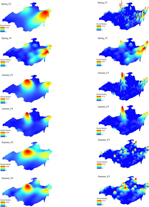
were obtained (Figure 4). According to the seasonal KDE
where Dtr is the true density for an active fire point i, k is maps, the densities of active grassland fire points show
the number of adaptive nearest neighbor points, r is the different spatial distribution patterns, although all of
distance to the kth nearest neighbor point at the sample them show the clustering characteristic (Figure 4). In
point i, and A(r ) i, k is the circular area with the radius r. all seasons, the density surfaces calculated by the RDmean
This procedure emphasizes the estimation in the vicinity method have spikier than those calculated with other
of each active fire position, rather than estimating the methods. In contrast, the results calculated with the the-
density of the whole samples in the study area. According oretical bandwidth method are the smoothest surfaces.
to the number of observed points in spring, summer, and With Williamson and Ripley’s K methods, the degrees of
autumn, k is defined as 10, 20, and 30, respectively. The surface smoothness are medium. The difference of max-
mean true density value of each active fire point is calcu- imum density values of different methods is substantial
lated by function (7) at these three neighbor numbers. Com- in all seasons. The method with the biggest density value
bined with equations (6) and (7), the minimum value of is RDmean, followed by Ripley’s K, Williamson, and The-
MISE shows the best bandwidth of KDE for active grassland oretical bandwidths. The estimated density value nega-
fire points. tively correlates to the value of bandwidth, and the
surface smoothness is positively correlated with the
bandwidth value. Thus, with increasing values of band-
width, the density surfaces become smoother, and the
4 Results maximum density values become smaller.
An accuracy assessment approach is added to select
Using the analysis tool of Ripley’s K, the spatial distribu- the surface which better expresses the fire occurrence
tion pattern of grassland fire events was investigated in distribution. In the measurements of the density esti-
spring, autumn, and summer. The same distribution mator using MISE, the true density of each active grass-
characteristic of the fire points is found to be spatially land fire point was calculated by averaging the value
clustered in these three seasons (Figure 3). For the values with function (7) at 10, 20, and 30 neighbor distances
of ExpectedK greater than those of HiconfEnv, the statis- of each fire event. The density estimation of each active
tical tests show that the cluster distributions are signifi- grassland fire point was derived from the density sur-
cant. The largest DiffK values, which indicate the most faces of the four methods in spring, autumn, and summer.
pronounced distance of spatial processes promoting clus- The MISE values of the four methods in all seasons are
tering, are 99, 82, and 80 km in spring, autumn, and shown in Table 4. The differences in MISE among the var-
summer, respectively. In this circumstance, half of the ious bandwidths of the four methods are quite large. Rip-
value of maximum DiffK can be applied as the bandwidth ley’s K method for calculating bandwidth has the lowest
of KDE that represents the clustering characteristic of the MISE values among the methods in spring, autumn, and
spatial distribution pattern of active grassland fires in the summer. The MISE shows that the kernel density with
three seasons. Ripley’s K method gives the best density estimation of
Parameters related to the bandwidth calculations grassland fires in high, medium, and low concentration
and the values of the bandwidth calculated according scenes.
to the previous functions (2)–(4) with the grassland Therefore, the continuous spatial density surfaces
active fires are presented in detail in Tables 2 and 3. of grassland fire in different concentration scenes were
The differences among these bandwidth selection methods obtained as shown in Figure 4(F5). These density surfaces
are obvious. In all seasons, the bandwidths of the theore- can be used in grassland fire management practice and
tical bandwidth method are largest, and the values of risk research.802 Zhen Shuo et al.
Figure 3: The curves of Ripley’s K function for active grassland fire events in spring (a), autumn (b), and summer (c) in the study area.
5 Discussion KDE. We found that the bandwidth selection of Ripley’s
K method performed better than the other methods in
Choosing the suitable bandwidth is very critical because high, medium, and low concentration scenes of our sam-
it determines the range of variation of the estimation in ples. The previous methods that considered the sample
KDE [21]. These four bandwidth selection methods show and region size are reasonable because the amount of the
different abilities in calculating the density values of observed points has a relationship with the informationDensity of grassland fire points with KDE 803
Table 2: Parameters related to bandwidth calculations for different area and the sample size with the other methods. When
methods using the bandwidth selection method of Ripley’s K in
other studies, the correction method should be consid-
Parameter Value ered to increase the accuracy of the estimated density
Total size of the study area (A) 252,948 km2 surface, especially at the edge of the study area.
Total number of polygons 13 The best bandwidth selection by the MISE method is
Mean polygon size 19,594 km2 affected by the true density of samples. These two things
Total number of active fire events in Spring (N) 2639
cannot be acquired exactly. For the expert, these two
Total number of active fire events in Autumn (N) 1505
Total number of active fire events in summer (N) 406
things can also be presented by intuitive graphics in
Figure 4. Thus, the three-dimensional graph is an effec-
tive method to achieve the objective. In the measure-
ments of the accuracy of KDE using MISE, the neighbor
Table 3: The values of bandwidths for different methods number or the radius size is a critical factor in the identi-
fication of the true density of the samples. To decrease
Method Spring Autumn Summer the deviation of true densities of active grassland fire
(km) (km) (km) points, the mean densities of each sample at 10, 20,
Theoretical bandwidth 197 197 197 and 30 neighbor distances, which are also subjective,
(function 2) were applied in this study. The true density of samples
RDmean (function 3) 10 13 25 cannot be known, so expert knowledge of the study area
Williamson (function 4) 71 79 103
is needed.
Ripley’s K (function 5) 49.5 41 40
It is a fact that the number of samples and the dis-
tribution pattern affect the degree of smoothing. In our
study, the sample points of fire filtered by grassland
content. If the amount of sample points is more, which represent a discontinued part of the area, and the distri-
represents a large informative dataset, a smaller band- bution characteristic is a cluster. If the samples are gene-
width is more suitable for avoiding over smooth and loss rated for the whole area, Ripley’s K function must be
of the variability in the estimation. In contrast, if the used first for examining the distribution characteristic.
amount of sample points is small, which represents a When the ObservedK of the specific distance is greater
minor informative dataset, a larger bandwidth is more than the ExpectedK and HiConfEnv, the distribution char-
proper because a smaller bandwidth will cause the esti- acteristic is a significant cluster and the density of these
mated density that has little contact with neighbor points samples can be estimated by our method. If the ObservedK
[32]. In essence, these bandwidth selection methods repre- values are less than the confidential envelopes (LwconfEnv,
sent the concentration of the samples in a specific area, and HiconfEnv), a bias is generated between the samples and
the difference in spatial distribution pattern is neglected. In our methods because the sample distribution is dispersed
spatial datasets, especially for wildland fire samples, the or random. In this situation, the bandwidth selection
clustering characteristic is the main distribution pattern, method of Ripley’s K may not be better for calculating
and these samples have the characteristic of spatial auto- the kernel density surface. The previous bandwidth selec-
correlation. The bandwidth selection method of KDE by tion methods, especially RDmean and Williamson, may also
Ripley’s K can express the character of the distribution be used. However, it is important to apply this new band-
pattern. width selection method in many other studies because
In this study, the boundary correction method in pro- clustering is one of the important characteristics of spatial
cess of applying Ripley’s K was not considered. In this elements.
case, the neighbor number of samples near the edge was The effect of KDE is to calculate the density of sam-
underestimated. Increasing the number of samples out- ples for converting point data into continuous data.
side the study area is one method to rectify this situation. When calculating the densities with our method, the
Another method is to reduce the analyzed area and make type of spatial distribution of points should be calculated
some samples that occur outside of the reduced area. In first. If the spatial distribution type of points is a cluster,
this research, the previous three methods of bandwidth the optimal bandwidth (half of the DiffK) for the dataset
selection do not have the requirement of boundary cor- will be calculated with Ripley’s K. However, other methods
rection. When applying Ripley’s K function, the boundary should be used to calculate the bandwidth of the KDE
correction was neglected to maintain consistency of the map.804 Zhen Shuo et al. Figure 4: The KDE maps in spring, autumn, and summer, according to different bandwidth selection methods (F2: Theoretical bandwidth, function 2; F3: RDmean, function 3; F4: Williamson, function 4; F5: Ripley’s K, function 5).
Density of grassland fire points with KDE 805
Table 4: Mean integrated squared error (MISE) for different band- Data availability statement: Only freely and publicly
widths of kernel estimates in all seasons available datasets were used in this study. Data sources
were described in the paper.
Method MISE
Spring Autumn Summer
Theoretical bandwidth (function 2) 108.30 34.67 2.83
RDmean (function 3) 92.06 32.40 5.49 References
Williamson (function 4) 81.32 20.10 2.60
Ripley’s K (function 5) 68.17 11.23 2.47
[1] Hao WM, Liu MH. Spatial and temporal distribution of tropical
biomass burning. Global Biogeochem Cy. 1994;8(4):495–503.
doi: 10.1029/94gb02086.
[2] Noymeir I. Interactive effects of fire and grazing on structure
6 Conclusion and diversity of mediterranean grasslands. J Veg Sci.
1995;6(5):701–10. doi: 10.2307/3236441.
[3] Ojima DS, Schimel DS, Parton WJ, Owensby CE. Long-term and
In this study, the eastern Inner Mongolia Autonomous
short-term effects of fire on nitrogen cycling in tallgrass
Region of China, one of the main regions in the Asian prairie. Biogeochemistry. 1994;24(2):67–84. doi: 10.1007/
grassland that was significantly disturbed by grassland bf02390180.
fires, was selected as the study area. The MODIS Terra [4] Oom D, Pereira JMC. Exploratory spatial data analysis of global
and Aqua daily active fire product data (MOD14A1 and MODIS active fire data. Int J Appl Earth Obs. 2013;21:326–40.
doi: 10.1016/j.jag.2012.07.018.
MYD14A1) belonging to this region were downloaded
[5] Chuvieco E, Aguado I, Yebra M, Nieto H, Salas J, Pilar Martin M,
from LP-DAAC. As a nonparametric method for obtaining et al. Development of a framework for fire risk assessment
continuous surfaces from point observations, KDE has using remote sensing and geographic information system
been widely used to convert point-based data into den- technologies. Ecol Model. 2010;221(1):46–58. doi: 10.1016/
sity maps and to decrease the positional inaccuracy at the j.ecolmodel.2008.11.017.
same time. To find an adaptive bandwidth for fitting the [6] Amatulli G, Perez-Cabello F, de la Riva J. Mapping lightning/
human-caused wildfires occurrence under ignition point
grassland fire events and the study area, a bandwidth
location uncertainty. Ecol Model. 2007;200(3–4):321–33.
selection method on the basis of Ripley’s K function, doi: 10.1016/j.ecolmodel.2006.08.001.
which considered the clustering characteristic of the [7] Pew KL, Larsen CPS. GIS analysis of spatial and temporal
grassland fire events distribution pattern, was developed. patterns of human-caused wildfires in the temperate rain
It demonstrated that the developed bandwidth selection forest of Vancouver Island, Canada. Forest Ecol
Manag. 2001;140(1):1–18. doi: 10.1016/s0378-1127(00)
method is better than the previous methods in high,
00271-1.
medium, and low concentration scenes. Applying this [8] Koutsias N, Kalabokidis KD, AllgÖwer B. Fire occurrence pat-
method can promote wildland fire management in areas terns at landscape level: beyond positional accuracy of igni-
that are more prone to fire damage. Our approach pro- tion points with kernel density estimation methods. Nat
vides a general bandwidth selection method for KDE in Resour Model. 2004;17(4):359–75. doi: 10.1111/j.1939-
different studies as long as the samples have the clus- 7445.2004.tb00141.x.
[9] Martinez-Fernandez J, Chuvieco E, Koutsias N. Modelling long-
tering characteristics of a distribution pattern.
term fire occurrence factors in Spain by accounting for local
variations with geographically weighted regression. Nat
Funding information: This work was supported by the Hazard Earth Syst. 2013;13(2):311–27. doi: 10.5194/nhess-13-
National Natural Science Foundation of China under Grant 311-2013.
[number 41977407 and 41571489]; Jilin Provincial Science [10] Zhang ZX, Feng ZQ, Zhang HY, Zhao JJ, Yu S, Du W. Spatial
distribution of grassland fires at the regional scale based on
and Technology Development Project (20190101025JH).
the MODIS active fire products. Int J Wildland Fire.
2017;26(3):209–18. doi: 10.1071/wf16026.
Author contributions: Z.X.Z. proposed the idea, J.Y.Z. and [11] Waller LA, Gotway CA. Applied spatial statistics for public
S.Z. conducted data collection and experimental ana- health data. Hoboken, New Jersey, USA: John Wiley & Sons,
lysis, and J.J.Z. supervised the experiment. S.Z. wrote Inc.; 2004.
the manuscript. All the authors had read the manuscript [12] Gatrell AC, Bailey TC, Diggle PJ, Rowlingson BS. Spatial point
pattern analysis and its application in geographical epide-
and agreed to submit it.
miology. T I Brit Geogr. 1996;21(1):256–74. doi: 10.2307/
622936.
Conflict of interest: The authors do not have any possible [13] Steiniger S, Hunter AJS. A scaled line-based kernel density
conflicts of interest. estimator for the retrieval of utilization distributions and home806 Zhen Shuo et al.
ranges from GPS movement tracks. Ecol Inform. 2013;13:1–8. MYD14A2) products for mapping fires in the fynbos biome.
doi: 10.1016/j.ecoinf.2012.10.002. Int J Wildland Fire. 2008;17(2):166–78. doi: 10.1071/wf06040.
[14] Yu W, Ai T, Shao S. The analysis and delimitation of central [26] Giglio L, Descloitres J, Justice CO, Kaufman YJ. An enhanced con-
business district using network kernel density estimation. textual fire detection algorithm for MODIS. Remote Sens Environ.
J Transp Geogr. 2015;45:32–47. doi: 10.1016/ 2003;87(2–3):273–82. doi: 10.1016/s0034-4257(03)00184-6.
j.jtrangeo.2015.04.008. [27] Giglio L, van der Werf GR, Randerson JT, Collatz GJ,
[15] Gonzalez-Olabarria JR, Mola-Yudego B, Coll L. Different factors Kasibhatla P. Global estimation of burned area using MODIS
for different causes: analysis of the spatial aggregations of fire active fire observations. Atmos Chem Phys. 2006;6:957–74.
ignitions in catalonia (Spain). Risk Anal. 2015;35(7):1197–209. doi: 10.5194/acp-6-957-2006.
doi: 10.1111/risa.12339. [28] Morisette JT, Giglio L, Csiszar I, Setzer A, Schroeder W,
[16] Kuter N, Yenilmez F, Kuter S. Forest fire risk mapping by kernel Morton D, et al. Validation of MODIS active fire detection
density estimation. Croat J For Eng. 2011;32(2):599–610. products derived from two algorithms. Earth Interact.
[17] Li YP, Zhao JJ, Guo XY, Zhang ZX, Tan G, Yang JH. The influence 2005;9:1–25.
of land use on the grassland fire occurrence in the [29] Giglio L. MODIS collection 5 active fire product user’s guide
Northeastern Inner Mongolia autonomous region, China. version 2.5. College Park, MD: University of Maryland; 2013.
Sensors (Basel). 2017;17(3):437. doi: 10.3390/s17030437. p. 1–61.
[18] Silverman BW. Density estimation for statistics and data [30] He C, Gong YX, Zhang SY, He TF, Chen F, Sun Y, et al. Forest fire
analysis. London, UK: Chapman & Hall; 1986. division by using MODIS data based on the temporal-spatial
[19] Kuter S, Usul N, Kuter N. Bandwidth determination for kernel variation law. Spectrosc Spect Anal. 2013;33(9):2472–7.
density analysis of wildfire events at forest sub-district scale. doi: 10.3964/j.issn.1000-0593(2013)09-2472-06.
Ecol Model. 2011;222(17):3033–40. doi: 10.1016/ [31] Boer MM, Sadler RJ, Wittkuhn RS, McCaw L, Grierson PF. Long-
j.ecolmodel.2011.06.006. term impacts of prescribed burning on regional extent and
[20] de la Riva J, Perez-Cabello F, Lana-Renault N, Koutsias N. incidence of wildfires-Evidence from 50 years of active fire
Mapping wildfire occurrence at regional scale. Remote management in SW Australian forests. Forest Ecol Manag.
Sens Environ. 2004;92(3):363–9. doi: 10.1016/ 2009;259(1):132–42. doi: 10.1016/j.foreco.2009.10.005.
j.rse.2004.06.022. [32] Koutsias N, Balatsos P, Kalabokidis K. Fire occurrence zones:
[21] Worton BJ. Kernel methods for estimating the utilization dis- kernel density estimation of historical wildfire ignitions at the
tribution in home-range studies. Ecology. 1989;70(1):164–8. national level, Greece. J Maps. 2014;10(4):630–9.
doi: 10.2307/1938423. doi: 10.1080/17445647.2014.908750.
[22] Bailey TC, Gatrell AC. Interactive spatial data analysis. Essex: [33] Isham V, Northrop P. Statistical analysis of spatial point
Longman; p. 413. patterns. Devon, England: Exeter EX4 4QJ; 2003.
[23] Williamson D, Mclafferty S, Goldsmith V, Mollenkopf J, [34] Ripley BD. The second-order analysis of stationary point pro-
Mcguire PA. Better method to smooth crime incident data. cesses. J Appl Probab. 1976;13(2):255–66. doi: 10.2307/3212829.
ESRI ArcUser Magazine. California, USA: RedLands; [35] Besag J. Efficiency of pseudolikelihood estimation for simple
1999 Jan–Mar. gaussian fields. Biometrika. 1977;64(3):616–8. doi: 10.2307/
[24] Telesca L, Amatulli G, Lasaponara R, Lovallo M, Santulli A. 2345341.
Time-scaling properties in forest-fire sequences observed [36] Katkovnik V, Shmulevich I. Kernel density estimation with
in Gargano area (southern Italy). Ecol Model. adaptive varying window size. Pattern Recogn Lett.
2005;185(2–4):531–44. doi: 10.1016/ 2002;23(14):1641–8. doi: 10.1016/s0167-8655(02)00127-7.
j.ecolmodel.2005.01.009. [37] Seaman DE, Powell RA. An evaluation of the accuracy of kernel
[25] de Klerk H. A pragmatic assessment of the usefulness of the density estimators for home range analysis. Ecology.
MODIS (Terra and Aqua) 1 km active fire (MOD14A2 and 1996;77(7):2075–85. doi: 10.2307/2265701.You can also read