Incorporating Queueing Dynamics into Schedule-Driven Traffic Control
←
→
Page content transcription
If your browser does not render page correctly, please read the page content below
Proceedings of the Thirtieth International Joint Conference on Artificial Intelligence (IJCAI-21)

        Incorporating Queueing Dynamics into Schedule-Driven Traffic Control

                         Hsu-Chieh Hu1 , Allen M. Hawkes1 and Stephen F. Smith1,2
                                1
                                  Rapid Flow Technologies, Inc., Pittsburgh, PA
                                  2
                                    Carnegie Mellon University, Pittsburgh, PA
                            {hsuchieh, allen}@rapidflowtech.com, sfs@cs.cmu.edu

                          Abstract                                             and approaching platoons). This aggregate representation en-
                                                                               ables generation of near-optimal timing plans for individual
     Key to the effectiveness of schedule-driven ap-                           intersections in real-time, which are then shared with neigh-
     proaches to real-time traffic control is an ability to                    boring intersections to achieve network level coordination.
     accurately predict when sensed vehicles will arrive                       Original work demonstrated substantial traffic flow efficiency
     at and pass through the intersection. Prior work in                       improvements over statically optimized timing plans in ac-
     schedule-driven traffic control has assumed a static                      tual field test experiments [Smith et al., 2013]; and subse-
     vehicle arrival model. However, this static predictive                    quent work has explored the further advantages of incorpo-
     model ignores the fact that the queue count and the                       rating multi-modal traffic flows [Xie et al., 2014], integrating
     incurred delay should vary as different partial signal                    with queue management objectives [Hu and Smith, 2017a;
     timing schedules (i.e., different possible futures) are                   Hu and Smith, 2017b], exploiting higher fidelity predic-
     explored during the online planning process. In this                      tive models [Goldstein and Smith, 2019], upstream prop-
     paper, we propose an alternative arrival time model                       agation of congestion information [Hu and Smith, 2018;
     that incorporates queueing dynamics into this for-                        Hu and Smith, 2019], control of vehicle speed in connected
     ward search process for a signal timing schedule,                         vehicle setting [Hu et al., 2019], use of stochastic sampling
     to more accurately capture how the intersection’s                         for modeling turning proportions [Dhamija et al., 2020], and
     queues vary over time. As each search state is gen-                       learning of model parameters [Hu and Smith, 2020]. Already
     erated, an incremental queueing delay is dynami-                          incorporating many of these advances, this schedule-driven
     cally projected for each vehicle. The resulting total                     traffic control technology is now deployed and operating in 8
     queueing delay is then considered in addition to the                      North American cities.
     cumulative delay caused by signal operations. We
     demonstrate the potential of this approach through                           Despite this success, there is room for further improvement.
     microscopic traffic simulation of a real-world road                       One key to the effectiveness of any schedule-driven traffic
     network, showing a 10 − 15% reduction in average                          control algorithm is an ability to accurately predict when the
     wait times over the schedule-driven traffic signal                        sensed vehicles will arrive at and pass through the intersection.
     control system in heavy traffic scenarios.                                All prior work in schedule-driven traffic control has assumed
                                                                               a static vehicle arrival model to make this prediction (as origi-
                                                                               nally proposed in [Xie et al., 2012a]). Initially, each vehicle
1   Introduction                                                               cluster is associated with a free-flow arrival time, computed
As traffic congestion in cities continues to increase, it is                   using a fixed free-flow speed estimate and the distance from
generally recognized that better optimization of traffic sig-                  vehicle sensor location to the intersection. In situations where
nals is crucial to future urban mobility, and this fact, to-                   queued vehicles are already present at the intersection, a delay
gether with emergence of ubiquitous sensing capabilities,                      proportional to the queue count (the number of the queued
has led to new thinking around real-time approaches to this                    vehicles) is added to the free-flow arrival time, using the cur-
long studied problem (e.g., [Wongpiromsarn et al., 2012;                       rent queue count that remains unchanged, and this delay is
Varaiya, 2013; El-Tantawy et al., 2013; Duncan et al., 2014;                   propagated to all vehicle clusters within the planning horizon.
Mitrovic et al., 2019; Smith, 2020]. One promising approach                    The summation of the queueing delay and the free-flow arrival
that has emerged in recent years and is aimed specifically                     time to the end of queue is thus taken as a prediction of the
at urban traffic control, has been referred to as schedule-                    estimated arrival time for each vehicle cluster.
driven traffic control. [Xie et al., 2012a; Xie et al., 2012b;                    One limitation of this static predictive model, however, is
Smith et al., 2013] This approach treats traffic control as a                  that it ignores the fact that the queue count and its incurred
decentralized, online planning process, exploiting a novel                     queueing delay should vary as different partial signal timing
formulation of the intersection control problem as a single-                   schedules (i.e., different possible futures) are explored during
machine scheduling problem (where input jobs are sequences                     the online planning process. More specifically, the vehicle
of spatially proximate vehicle clusters representing queues                    cluster’s arrival time incorporating queueing delay depends

                                                                        4076
Proceedings of the Thirtieth International Joint Conference on Artificial Intelligence (IJCAI-21)
on when the previously queued vehicles are discharged and
when it joins the queue, and this time can be better predicted
through the previous partial schedule’s state and its free-flow
arrival time. We would expect to be able to further boost the
performance of the traffic signal control system by introducing
the ability to predict queueing delay online in response to
observed traffic behavior.
In this paper, we propose an online queue prediction algo-
rithm that incorporates queueing dynamics into this forward
search process for a signal timing schedule. Our algorithm
computes a more accurate estimate of the delay a queued ve- Figure 1: The resulting control flow (S, CCF ) and the predicted
hicle will experience than static queue estimation techniques queue count Q at each search state: each block represents a vehicular
without increasing overall search complexity. As each search cluster. The shaded blocks represent the delayed clusters.
state is generated, an incremental queueing delay relative to
the previous queued vehicle within the horizon is projected,
based on the previous state, the free-flow arrival time, and the job and a forward-recursion dynamic programming search is
queue dissipation model. The resulting total queueing delay is executed in a rolling horizon fashion to continually generate
considered in addition to the original cumulative delay caused a phase schedule that minimizes the cumulative delay of all
by signal operations when evaluating alternative partial sched- clusters. In practice, the planning cycle is repeated every sec-
ules. With this extension, we are able to better capture not ond or two, to reduce the uncertainty associated with clusters
only how the intersection’s queues vary over time but also the and queues. The process constructs an optimal sequence of
impact of vehicle stops on cumulative delay at the intersec- clusters that maintains the ordering of clusters along each road
tion. We demonstrate the potential of this approach through segment m, and each time a phase change is implied by the
microscopic traffic simulation of a real-world road network, sequence.
showing a 10 − 15% reduction in average wait times in heavy Formally, the resulting control flow can be represented as a
traffic scenarios over a schedule-driven variant that is utilizing tuple (S, CCF ) shown in Figure 1, where S is a sequence of
the previous static predictive model. phase indices, i.e., (s1 , · · · , s|S| ), CCF contains the sequence
of clusters (c1 , · · · , c|S| ), ci ∈ C and the corresponding start-
ing time after being scheduled. More precisely, the delay that
2 Schedule-Driven Traffic Control P|S|
each cluster contributes to the cumulative delay k=1 d(ck )
As noted above about the schedule-driven approach, the essen- is
tial consequence of the single machine scheduling problem d(ck ) = |ck | · (ast − arr(ck )), (1)
formulation of [Xie et al., 2012b] is that traffic flows are
treated as sequences of clusters c over the planning (or pre- where ast is the actual start time that the vehicle is allowed to
diction) horizon. Each cluster c is defined as (|c|, arr, dep), pass through, which is determined by arr and permitted start
where |c|, arr and dep are number of vehicles, arrival time time (pst). For a partial schedule Sk , the corresponding state
and departure time respectively. Vehicles approaching an in- variables are defined as a tuple, (s, pd, t, d), where s is phase
tersection from the entry roads are clustered together if the index and pd is duration of the last phase, t is the finish time of
time gap between them is less than a pre-specified time inter- the kth cluster and d is the accumulative delay for all k clusters.
val (e.g., 1 second). The clusters then become the input jobs The state variable of Sk can be updated from Sk−1 , and the
that must be sequenced through intersection (i.e., the single corresponding pst for ck is equal to t + M inSwitch(s, i),
machine). Once a vehicle departs the intersection, it is sensed where M inSwitch(s, i) returns the minimum time required
and grouped into a new cluster by the downstream neighbor for switching from phase s to i and slti is the start-up lost time
intersection. The sequences of clusters provide short-term for clearing the queue in the phase i. The optimal sequence
∗
variability of traffic flows for optimization and preserve the (schedule) CCF is the one that incurs minimal delay for all
non-uniform nature of real-time flows. vehicles.
More specifically, the input to the online planning process
at the beginning of each planning cycle is a set C of phase 3 Incorporating Queueing Dynamics into
cluster sequences, where a phase is a compatible traffic move- Scheduling
ment pattern such as East-West traffic flow. A phase cluster
sequence CP,i for a given phase i is obtained by merging those 3.1 Queueing Delay
constituent road cluster sequences CR,m that can proceed con- Other than the delay caused by the signal operations, i.e.,
currently through the intersection and belong to the phase, d(c) = |c| · (ast − arr(c)), a cluster may experience an extra
where each CR,m consists of (|c|, arr, dep) triples that reflect delay, known as queueing delay, if the cluster’s constituent
each approaching or queued vehicle on entry road segment vehicles are forced to decelerate or stop due to queued vehicles
m and are ordered by increasing arr. The travel time on en- in front of them. In the static vehicle arrival model utilized
try road m defines a finite horizon (Hm ), and the prediction in previous work, this delay is considered to be proportional
horizon H is the maximum over all road segments. to current queue count (the number of the queued vehicles in
During planning, each cluster is viewed as a non-divisible front of the approaching cluster). This count is assumed to
4077Proceedings of the Thirtieth International Joint Conference on Artificial Intelligence (IJCAI-21)
Algorithm 1 Calculate qdinter and qdintra of c Algorithm 2 Calculate (pd, t, d) of Sk
Require: 1) pst, a0 , a1 , sk ; 2) (s, pd, t, d) of Sk−1 Require: 1) (s, pd, t, d) of Sk−1 ; 2) sk
1: i = sk ; c = next job of phase i; qdinter , qdintra = 0 1: i = sk ; c = next job of phase i
2: w = max(0, |c| − 1) . exclude the first vehicle of c 2: Compute qd, and update dep(c) and pst:
3: if pst > arr(c) and c is not queued then . c will stop a: pst = t + M inSwitch(s, i);
4: if s 6= i and arr(c) > t then . New phase starts b: (dep(c), qdinter , qdintra ) =Algorithm 1, given
5: qdintra = w · (a0 − a1 ) (pst, a0 , a1 ), input 1) and 2); . Queueing dynamics
6: dep(c) = dep(c) + a0 + max(0, w − 1) · a1 c: pst = pst + qdinter ; . insert qdinter if needed
7: else if arr(c) ≤ t then . Queue already exists 3: ast = max(arr(c), pst) . Actual start time of c
8: qdinter = a1 4: if s 6= i and pst > arr(c) then ast = ast + slti
9: dep(c) = dep(c) + w · a1 5: end if
10: end if 6: t = ast + dep(c) − arr(c) . Actual finish time of c
11: qdintra = qdintra + (w + 1)w/2 · a1 7: if s 6= i then pd = t − pst
12: end if 8: else pd = pd + (t − pst)
13: return (dep(c), qdinter , qdintra ) 9: end if
10: d = d + |c| · (ast − arr(c)) + qdintra . Total delay
11: return (pd, t, d)
persist throughout the planning horizon and is not recomputed
as different partial schedules are expanded.
To better capture the queueing dynamics in these situations, vehicles joining the queue experience an additional headway
we propose to incorporate an alternative vehicle arrival model a1 . Since the initial speed is small, a0 should be greater than
where queueing delay evolves as a function of different partial a1 . With this model, we can estimate how much delay a
signal timing schedules (i.e., different possible futures) that are queued vehicle will experience before being dissipated and
explored during the online planning process. More specifically, the headway relative to the previous queued vehicle. Although
as the search states representing different partial schedules the model can be extended to a more complicated polynomial
are expanded to incorporate the next approaching cluster, the or non-linear functional form, our experimental data shows
possibility of queuing delay is assessed. If the arr of the next that a linear model is sufficient to model dissipation. The
cluster to be added to the schedule, computed using a fixed parameters can be selected by field experiments or learned by
free-flow speed estimate and the distance from vehicle sensor online learning algorithms.
location to the intersection, is less than the finish time t of the To retain the efficiency of generating longer-horizon plans,
previous search state (i.e., the intersection departure time of we define two types of queueing delay for a vehicle cluster that
the previous cluster), then this cluster is determined to have contains multiple vehicles: 1) intra-cluster queueing delay and
joined the queue. In this case, the headway (i.e., the temporal 2) inter-cluster queueing delay. Intra-cluster queueing delay
gap between two adjacent queued vehicles) of all preceding is the delay experienced by all vehicles other than the first
vehicles in the queue ahead of the cluster is summed and added vehicles within the cluster, and it can cause the enlargement
to the cluster’s free-flow arr as the queueing delay, and arr of the cluster (i.e., dep(c) increases). Inter-cluster queueing
and dep of the vehicle clusters will be thus delayed. delay, alternatively, is the delay experienced by the first vehicle
To incorporate the queueing delay into the objective, a within the cluster if there are already one or more queued
queueing delay that is relative to ast is added to the origi- clusters in front of it, and the pst will be delayed. For the
nal cluster delay, and the total delay contributed by cluster c is example of Figure 1, the stop of cluster (2, 1) causes a qdinter
rewritten as between (2, 1) and (2, 2), and the stop of (2, 2) causes qdinter
between (2, 2) and (2, 3) and qdintra within (2, 3). With these
d(c) = |c| · (ast − arr(c)) + qd(c), (2) definitions, Equation 2 can be rewritten as
where qd(c) is the queueing delay of c and can be de deter- d(c) = |c| · (ast + qdinter − arr(c)) + qdintra , (4)
mined through the search process and a queue dissipation
model that will be introduced in the next section. where qdinter and qdintra are the inter-cluster and intra-
cluster queueing delay and qd(c) = |c| · qdinter + qdintra .
3.2 Queue Dissipation Model qdintra and qdinter can be calculated given a0 , a1 and the
state tuple (s, pd, t, d) by Algorithm 1.
The total queueing delay for a single vehicle due to the ex- In Algorithm 2, we describe how the search state Sk is
isting standing queue can be estimated using the following expanded from Sk−1 , given the previous tuple (s, pd, t, d),
relationship adopted from [Head, 1995]): based on a greedy realization of planned signal sequence.
qdtotal (Nq ) = a0 + a1 · (Nq − 1), a0 ≥ a1 ; Nq ≥ 1 (3) Algorithm 1 is executed at Line 2 of Algorithm 2, and then
qdinter , qdintra , and dep(c) are derived for revising pst and
where a0 and a1 are parameters that can be selected on the delay contribution accordingly. Then, ast is determined by
basis of the particular intersection and Nq is the number of the maximum of arr and pst at Line 3 of Algorithm 2. If arr
vehicles already in the queue. The interpretation of this model is less than pst, this means that the cluster will stop and the
is that a0 is a sum of the initial headway and residual start-up both types of queueing delay should be included. We consider
lost time for the second vehicle in the queue, and the following two cases after knowing the cluster will stop. First, if a cluster
4078Proceedings of the Thirtieth International Joint Conference on Artificial Intelligence (IJCAI-21)
joins an existing queue, then its qdintra is calculated based on Algorithm 3 Predict Q(Sk ) given Sk−1 and ck
the following theorem: Require: 1) Sk−1 ,Q(Sk−1 ); 2) ck−1 and ck
Theorem 1. If a cluster c joins an existing queue, the in- 1: l(Sk ) = 0;ptr = ck−1
curred queueing delay within the cluster is O(|c|2 ) and can 2: while max(phase start, arr(ck−1 )) < ast(ptr) do
be calculated by qdintra = (|c|−1)|c|
2 · a1 3: if t(ptr) < arr(ck ) then . check end time t of ptr
4: l(Sk ) = l(Sk ) + |ptr| . ptr is dissipated
Proof. The queueing delay experienced by the second vehicle 5: end if
within the cluster is a1 ; The one experienced by the third 6: ptr = previous cluster of the cluster ptr
vehicle is 2a1 contributed by the queueing delay from the 7: end while
previous vehicle and itself, and so on. qdintra experienced 8: Q(Sk ) = Q(Sk−1 ) + |ck−1 | − l(Sk )
by the vehicles within c other than the first vehicle is thus
a1 + · · · + (|c| − 1) · a1 = (|c|−1)|c|
2 · a1 .
(i.e., a start of a new phase), the queue count is 0 as well. c) If
Then, qdinter is set to a1 and added to pst when the cluster the cluster stops and a queue already exists, given the queue
joins an existing queue. Its contribution to the cumulative count of the previous state, then the queue count of the current
delay is |c| · a1 . Equation 4 can be rewritten as state is represented as
(|c| − 1)|c|
d(c) = |c| · ast + a1 − arr(c) + · a1 (5) Q(Sk ) = Q(Sk−1 ) + |ck−1 | − l(Sk ), (6)
2
Second, if a new phase has just started in the currently ex- where Q(Sk ) is the observed queue count of the partial sched-
panded search state, then the second vehicle within the added ule Sk for ck , and l(Sk ) is the number of dissipated vehicles
cluster will experience headway a0 instead of a1 and the rest between the arrivals of ck and ck−1 .
of vehicles will still experience a1 instead. Therefore, the More specifically, the number of the vehicles joining the
queueing delay needs to be offset by the difference (a0 − a1 ). queue at each state is simply |ck−1 | of the previous cluster
Note that there is no qdinter in this case since it is the first in the same road cluster sequence CR,m on road segment
cluster in the new phase. m. However, knowing the number of the dissipated vehicles
requires to count how many vehicles whose end times t fall
3.3 Online Planning with Queueing Delay within the range between two adjacent arrivals are dissipated.
In this section, we describe how to integrate queueing delay An algorithm that computes Q(Sk ) in the case c) is provided
into the online planning algorithm and predict the queue count. in Algorithm 3,
The goal is to improve traffic control performance by utilizing Since the extension does not generate additional states dur-
a more accurate predictive queueing model. ing the search, it retains the efficiency of scheduling with
First, before computing the schedule, we determine whether longer horizons, and the complexity is still polynomial in
a vehicle is queued or not given the snapshot of current queue |H| = H/δ, the number of time steps in H [Xie et al., 2012b],
count. Then, all vehicles approaching the intersection are given a time resolution δ.
clustered together based on the free-flow arr at their free-flow Currently, the baseline arr for calculating delay is assumed
speed. In other words, approaching vehicles are clustered to be arrival time of the vehicle cluster if moving according
according to their geometrical proximity. After clustering, we to the static arrival model. In the following section, a concept
delay arr of the queued clusters based on the snapshot by of minimum guaranteed queue is introduced to define the
adding Equation 3 according to the queue count they observe objective (cumulative delay) for taking both queueing delay
when joining the queue, and this delayed arr will serve as a and signal delay into consideration.
part of the initial state for building the schedule.
When computing the schedule, each cluster will be checked 3.4 Minimum Guaranteed Queue
if it joins a queue. If so, dep(c) of the free-flow clusters will
According to Equation 1, each cluster contributes a time differ-
be increased, and the queueing delay is computed to update
ence between the ast and the free-flow arr to the cumulative
pst and the objective as described in Algorithm 2 and 1 at
delay. After taking queueing delay into account, ast is offset
each expansion step of the search.The physical interpretation
by a queueing delay (equally a headway), i.e, qdinter , and
of this update is that the stop due to the current queue expands
qdintra are added according to Equation 4. In turn, the delay
the cluster duration dur by a1 · max(0, |c| − 1) and increases
contribution of each cluster should include the total queueing
the gap between clusters’ arrival time by qdinter .
delay caused by all previous queued vehicles other than the sig-
Since the previously queued clusters will depart the inter-
nal delay. However, to define the cluster delay correctly, arr
section at the ast = max(pst, arr(c)) that is determined by
should be a delayed arr in which we assume each cluster will
the schedule, we can predict the queue count at any future
experience its own minimum queue count if the corresponding
time points within the horizon H by tracking the number of
green phase persists.
the dissipated vehicles and the number of vehicles joining the
queue at each search state. Three cases mentioned in Algo- Definition 1 (Minimum Guaranteed Queue). Minimum Guar-
rithm 1 are necessarily considered for predicting the queue anteed Queue (MGQ) is the minimum queue count a moving
count: a) If the cluster does not stop, the queue count of this cluster observes when it joins the queue under an assumption
cluster is 0. b) If the cluster stops and a queue does not exist that the corresponding phase stays green until the cluster exits.
4079Proceedings of the Thirtieth International Joint Conference on Artificial Intelligence (IJCAI-21)
MGQ is used to specify arr of the cluster delay (i.e., Equa- 25
Queueing delay and queue count
tion 5) when both qdintra and qdinter are considered and Avg.
Average queueing delay (s)
Avg. w/ signal delay = 0
taken as a baseline to define delay. Meanwhile, the minimum 20 Avg. w/ signal delay > 0
queueing delay without any intervention of the traffic signal
can be calculated directly from MGQ. However, since MGQ is 15
irrelevant to any state transition, the solutions will only differ
by a constant if another baseline arr, e.g., arr at the free-flow 10
speed, is applied.
5
Theorem 2. The solutions of any baseline arr will only differ 1 2 3 4 5
Queue count when joining the queue
6
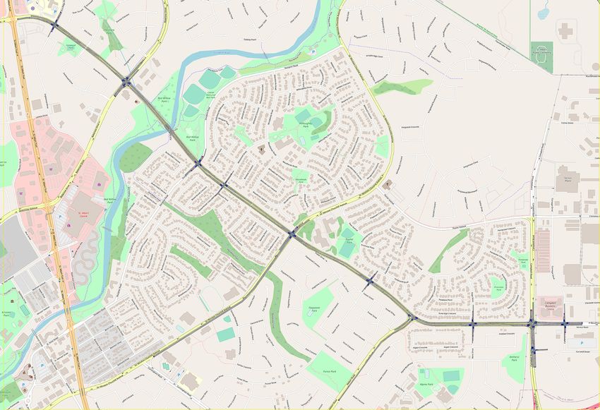
Figure 3: Map of the 11 in-
by a constant compared to the arr calculated with MGQ. tersections in the St. Albert,
Figure 2: The average queueing Canada
delay for different queue counts.
Proof. arr is not state-dependent due to the traffic signal
operations. Therefore, we can replace it with any baseline arr
without compromising the optimality of the solution. Since the headway parameters a0 and a1 are critical for
computing the queueing delay, setting them correctly could
Due to Theorem 2, we simply use the free-flow arr to affect how the queueing dynamics are modeled. We consider
compute the schedule without loss of optimality unless there a simple two-intersection model with 2-way, single lane, and
is a need for acquiring the actual cost of the schedule. multi-directional traffic flow as controlled experiments. The
source of traffic is assumed to be stationary and set to 500
4 Experimental Evaluation cars/hour. In Figure 2, three scenarios are plotted. We can see
that the three lines actually fit the queue dissipation model (i.e.,
In this section, we compare the above described online Equation 3) closely, which can be characterized by an intercept
queue prediction algorithm to three other real-time traffic (i.e., a0 ) and a slope (i.e., a1 ). The difference between them
control methods. First, we include the two most recent is in whether vehicles experience a signal delay or not. If
variants of the schedule-driven traffic control system: a) the signal delay is larger than 0, an additional start-up lost
The variant that ensures queueing stability (i.e., that queues time should be added to the average delay, leading to an upper
will not increase without bound) [Hu and Smith, 2017a; shift of the line. We use a linear function to approximate the
Hu and Smith, 2017b] serves as the primary benchmark since line without the signal delay, and the estimations of a0 and a1
this version has been proved to be effective in several North are approximately (5.8s, 2.4s). We then apply these values
America cities [Smith, 2020], and b) the more recent bi- to a larger complex network. For non-stationary traffic, a0
directional extension that utilizes the downstream congestion and a1 can be adjusted adaptively through tracking arrival and
information [Hu and Smith, 2018; Hu and Smith, 2019] is departure of vehicles. It is worth noting that the performance
also included as another point of comparison. We implement of this model shows the same trend as the following urban
new versions of each of these two extensions that incorporate network model.
online queue prediction. Second, we compare to a variant of
The network model we consider for a more complex sce-
backpressure adaptive control [Wongpiromsarn et al., 2012;
nario is based on the St. Albert neighborhood of Canada
Varaiya, 2013] that makes decisions based on the estimated
as shown in Figure 3. The network consists of 11 intersec-
queue count and ensures queueing stability. 1
tions that basically have multiple phases. It can be seen as
To evaluate our approach, we simulate performance on a a two-way corridor network. To explore how the proposed
two-intersection model and a real world network. The two- algorithm performs under different traffic patterns and de-
intersection model is used to estimate model parameters. The mands, we evaluate two traffic patterns: AM and PM rush
real world network is used to evaluate the performance of hour, and categorize traffic demand into three different groups:
planning with queueing delay in a larger complex real network low (AM/PM 116.18/66.55 cars/hour), medium (AM/PM
and real traffic pattern. The simulation model was developed 249.27/99.82 cars/hour), and high (AM/PM 332.36/133.10
in VISSIM, a commercial microscopic traffic simulation soft- cars/hour). The low demand data is extracted from the field
ware package. We assume that each vehicle has its own route data of St. Albert of 6-9am, 1/6/2020 - 1/8/2020, and ramped
as it passes through the network and measure how long a vehi- up to generate two other demands.
cle must wait for its turn to pass through the intersections (the
Table 1 shows that both versions of the proposed method
delay). Tested traffic volume is averaged over sources at net-
are basically comparable except that the one combining with
work boundaries. To assess the performance boost provided by
benchmark (i.e., ensure queueing stability) performs better
the proposed algorithm, we measure the average waiting time
than the other by 2.4% under the AM high demand case. In the
of all vehicles over five runs. All simulations run for 1 hour of
following results, we mainly consider this variant to present
simulated time. Results for a given experiment are averaged
our evaluation. It shows the online queue prediction to yield a
across all simulation runs with different random seeds.
delay improvement over the benchmark and the bi-directional
1
Note also that previous research with the baseline schedule- extension of about 13%/19% and an improvement of about
driven approach has shown its comparative advantage over prior 20% over backpressure control for the AM high traffic demand
online planning approaches to real-time traffic signal control [Xie et case. For the number of stops, the improvements are 24%,
al., 2012a]. 23% and 48% respectively. For low and medium traffic, the de-
4080Proceedings of the Thirtieth International Joint Conference on Artificial Intelligence (IJCAI-21)
Average Delay (second) and Number of Stops
Benchmark Bi-directional Planning with qd (benchmark) Planning with qd (bi-direc.) Backpressure
mean std. stop no. std. mean std. stop no. std. mean std. stop no. std. mean std. stop no. std mean std. stop no. std
AM High 95.55 95.87 3.89 7.34 104.57 103.94 3.66 7.19 84.77 81.10 2.96 4.33 86.83 82.12 3.03 4.53 105.61 118.63 5.68 10.94
AM Medium 64.86 60.98 1.74 1.80 62.96 57.23 1.65 1.62 56.04 52.94 1.60 1.50 56.64 53.31 1.61 1.54 59.29 55.39 1.73 1.67
AM Low 54.11 53.68 1.40 1.25 53.59 52.87 1.44 1.3 49.54 49.41 1.37 1.22 49.37 49.57 1.38 1.25 52.16 51.66 1.39 1.24
PM High 50.08 50.36 1.29 1.11 49.57 49.73 1.33 1.21 47.75 48.78 1.29 1.13 48.91 49.12 1.32 1.15 51.97 53.5 1.33 1.15
PM Medium 47.20 49.67 1.25 1.10 46.54 49.16 1.23 1.19 45.73 47.31 1.22 1.07 46.22 47.55 1.23 1.09 51.02 53.63 1.25 1.07
PM Low 44.58 48.26 1.20 1.01 43.85 48.32 1.19 1.01 46.11 48.80 1.20 1.02 45.78 48.60 1.19 1.18 55.20 58.03 1.21 1.02
Table 1: The mean and standard deviation (std.) of delay and number of stops (stop no.) under different scenarios.
lay and the stops of the proposed approach are generally better 2nd Cluster 3rd Cluster
Avg. [±3s] [±5s] h(second) Avg. [±3s] [±5s] h(second)
than the three approaches. The online queue prediction en-
Phase 2 1.92 1.22 1.11 26.91 1.80 1.24 1.09 41.16
abling planning with the queueing delay prevents the decision Phase 8 1.53 0.73 0.63 20.92 1.94 0.94 0.86 29.53
making from falling into short-sighted decisions and allows it
to outperform backpressure, which only utilizes current queue Table 2: RMSE and lookahead h of using 2nd and 3rd cluster to pre-
counts to make decisions. On the other hand, compared to the dict queue count at Boudreau-SWC and their corresponding average
benchmark, which is actually comparable to the bi-directional queue count
extension, taking the queueing delay into account more ac-
curately captures realistic traffic variation and improves the
through planning. For example, compared to the backpressure,
schedule. Moreover, from the AM high demand case, we can
although the proposed approach has longer queues at the first
see that maintaining queueing stability and using prediction
three roads of Boudreau-Bellerose, the reduction of the queue
are both crucial for reducing congestion.
count on the forth road is significant in return. It is the same
For the PM rush hour, although the demand is not as large for the third road at Boudreau-Campbell.
as the AM rush hour, several dominating roads are present According to Algorithm 3, future queue count is predicted
instead of a single main road like the AM rush, requiring during generating schedule and tracking arrivals/departures of
better coordination among the intersections. Because of the the clusters. In Table 2, two comparisons on different phases
lower demand, the backpressure approach is not able to re- (i.e., 2 and 8) at Boudreau-Sir Winston Churchill (SWC) in-
duce delay through the simple queueing policy. Contrarily, tersection are made. We take the second and the third cluster
the backpressure’s weakness to coordinate intersections is to (i.e., c2 and c3 ) as predictions of the future queue count. Due
worsen the delay of entire network, so it has the largest de- to the uncertainty of arrival time, the measured queue count
lay among four approaches under the PM low demand. The that is within a window (e.g., ±3 or ±5 second) and has the
proposed online queue prediction is generally better than the smallest error is chosen to compute root-mean-square error
benchmark and the bi-directional extension, even in PM rush (RMSE). The prediction error is around 1 vehicle, and the
hour it has shorter queues. The benefits come from the fact average lookahead h(second) could be up to 40 second.
that the proposed vehicle arrival model is more accurate at
predicting arrival times. 5 Conclusion
Figure 4 also shows the average queue counts of two
bottleneck intersections, Boudreau-Bellerose and Boudreau- In this work, we considered the limitations of prior approaches
Campbell, under the AM high demand scenario. The average to schedule-driven traffic control that rely on a static arrival
queue count of four roads at both intersections are shown. model without regard to the fact that the queue count and the
The proposed approach has the shortest queue, compared to incurred delay should vary as different partial signal timing
the benchmark and the backpressure approach respectively. schedules are explored during the online planning process.
As can be seen, the use of online queue prediction reduces An online queue prediction algorithm is proposed to achieve
the queue count and balances the queues among four roads better delay and number of stops in circumstances of high
traffic demand. In this algorithm, each scheduling agent com-
putes queueing delay of each cluster dynamically, as states are
expanded during the search process, given the previous state
25
Average Queue at Boudreau-Bellerose 30
Average Queue at Boudreau-Campbell
and the free-flow arrival time, and predicts the arrival time
Benchmark Benchmark
dynamically. Experimental results showed that the proposed
Average Queue Count
Average Queue Count
Planning with QD 25 Planning with QD
20
(bench.) (bench.)
Backpressure 20 Backpressure approach improves cumulative delay overall in comparison to
15
15
the schedule-driven traffic control approaches using a static
10
10
vehicle arrival model and a backpressure approach, and that
5
5
solutions provide substantial gain in highly congested scenar-
0 0
ios.
Phase 2 Phase 6 Phase 4 Phase 8 Phase 2 Phase 6 Phase 4 Phase 8
(a) Boudreau-Bellerose (b) Boudreau-Campbell Acknowledgements
Stephen F. Smith’s work was supported in part by the Na-
Figure 4: Average queue counts at 2 most congested intersections in tional Science Foundation, under award #2038612, and the
the network Mobility21 University Transportation Center at CMU.
4081Proceedings of the Thirtieth International Joint Conference on Artificial Intelligence (IJCAI-21)
References [Mitrovic et al., 2019] Nikola Mitrovic, Igor Dakic, and
[Dhamija et al., 2020] Srishti Dhamija, Alolika Gon, Pradeep Aleksandar Stevanovic. Combined alternate-direction
lane assignment and reservation-based intersection control.
Varakantham, and William Yeoh. Online traffic signal
IEEE Transactions on Intelligent Transportation Systems,
control through sample-based constrained optimization.
21(4):1779–1789, 2019.
In Proceedings of the International Conference on Auto-
mated Planning and Scheduling, volume 30, pages 366– [Smith et al., 2013] Stephen F. Smith, Gregory J. Barlow,
374, 2020. Xiao-Feng Xie, and Zachary B. Rubinstein. Smart urban
signal networks: Initial application of the surtrac adaptive
[Duncan et al., 2014] Gary Duncan, Larry K. Head, and traffic signal control system. In Proceedings of the Interna-
R. Puvvala. Multi-modal intelligent traffic signal system- tional Conference on Automated Planning and Scheduling,
safer and more efficient intersections through a connected pages 434–442, 2013.
vehicle environment. IMSA Journal, 52(5), 2014.
[Smith, 2020] Stephen F. Smith. Smart infrastructure for fu-
[El-Tantawy et al., 2013] Samah El-Tantawy, Baher Abdul- ture urban mobility. AI Magazine, 41(1):5–18, 2020.
hai, and Hossam Abdelgawad. Multiagent reinforcement
learning for integrated network of adaptive traffic signal [Varaiya, 2013] Pravin Varaiya. Max pressure control of a net-
controllers (marlin-atsc): methodology and large-scale ap- work of signalized intersections. Transportation Research
plication on downtown toronto. IEEE Transactions on In- Part C: Emerging Technologies, 36:177–195, 2013.
telligent Transportation Systems, 14(3):1140–1150, 2013. [Wongpiromsarn et al., 2012] Tichakorn Wongpiromsarn,
[Goldstein and Smith, 2019] Rick Goldstein and Stephen F Tawit Uthaicharoenpong, Yu Wang, Emilio Frazzoli,
and Danwei Wang. Distributed traffic signal control for
Smith. Expressive real-time intersection scheduling. In
maximum network throughput. In 2012 15th International
Proceedings of the AAAI Conference on Artificial Intelli-
IEEE Conference on Intelligent Transportation Systems,
gence, volume 33, pages 9882–9883, 2019.
pages 588–595. IEEE, 2012.
[Head, 1995] Larry K. Head. Event-based short-term traffic [Xie et al., 2012a] Xiao-Feng Xie, Stephen F. Smith, and Gre-
flow prediction model. Transportation Research Record, gory J. Barlow. Schedule-driven coordination for real-time
1510:45–52, 1995. traffic network control. In ICAPS, 2012.
[Hu and Smith, 2017a] Hsu-Chieh Hu and Stephen F. Smith. [Xie et al., 2012b] Xiao-Feng Xie, Stephen F. Smith, Liang
Coping with large traffic volumes in schedule-driven traffic Lu, and Gregory J. Barlow. Schedule-driven intersection
signal control. In Proceedings of the International Confer- control. Transportation Research Part C: Emerging Tech-
ence on Automated Planning and Scheduling, pages 154– nologies, 24:168–189, 2012.
162, 2017.
[Xie et al., 2014] Xiao-Feng Xie, Stephen F. Smith, and Gre-
[Hu and Smith, 2017b] Hsu-Chieh Hu and Stephen F. Smith. gory J. Barlow. Real-time traffic control for sustainable
Softpressure: a schedule-driven backpressure algorithm for urban living. In 17th International IEEE Conference on In-
coping with network congestion. In Proceedings of the 26th telligent Transportation Systems (ITSC), pages 1863–1868,
International Joint Conference on Artificial Intelligence, 2014.
pages 4324–4330, 2017.
[Hu and Smith, 2018] Hsu-Chieh Hu and Stephen F. Smith.
Bi-directional information exchange in decentralized
schedule-driven traffic control. In Proceedings of the inter-
national conference on autonomous agents and multiagent
systems, pages 1962–1964, 2018.
[Hu and Smith, 2019] Hsu-Chieh Hu and Stephen F. Smith.
Using bi-directional information exchange to improve de-
centralized schedule-driven traffic control. In Proceedings
of the International Conference on Automated Planning
and Scheduling, volume 29, pages 200–208, 2019.
[Hu and Smith, 2020] Hsu-Chieh Hu and Stephen F. Smith.
Learning model parameters for decentralized schedule-
driven traffic control. In Proceedings of the International
Conference on Automated Planning and Scheduling, vol-
ume 30, pages 531–539, 2020.
[Hu et al., 2019] Hsu-Chieh Hu, Stephen F. Smith, and Rick
Goldstein. Cooperative schedule-driven intersection con-
trol with connected and autonomous vehicles. In 2019
IEEE/RSJ International Conference on Intelligent Robots
and Systems (IROS), pages 1668–1673. IEEE, 2019.
4082You can also read