KAT-5: Robust systems for autonomous vehicle navigation in challenging and unknown terrain
←
→
Page content transcription
If your browser does not render page correctly, please read the page content below

KAT-5: Robust systems for autonomous vehicle navigation in
               challenging and unknown terrain

 Paul G. Trepagnier∗, Jorge Nagel†, Powell M. Kinney, Cris Koutsougeras, and Matthew Dooner

                                                          Abstract

             Kat-5 was the fourth vehicle to make history in DARPA’s 2005 Grand Challenge,
             where for the first time ever, autonomous vehicles were able to travel through 100
             miles of rough terrain at average speeds greater than 15 mph. In this paper, we
             describe the mechanisms and methods that were used to develop the vehicle. We
             describe the main hardware systems with which the vehicle was outfitted for navi-
             gation, computing, and control. We describe the sensors, the computing grid, and
             the methods that controlled the navigation based on the sensor readings. We also
             discuss the experiences gained in the course of the development and provide high-
             lights of actual field performance.

1        Introduction

The DARPA Grand Challenge aimed at fostering the development of a completely full-scale au-
tonomous vehicle that would live up to the challenge of high-speed navigation through challenging
and unknown terrain. Organized by DARPA (Defense Advanced Research Projects Agency), the
Grand Challenge was first held in 2004, but by the conclusion of the event, no vehicle had com-
pleted more than 7 miles of the prescribed course. Even with such poor results, DARPA sponsored
the Grand Challenge again in 2005. This time their hopes were justified as not one, but five vehi-
cles finished the 132-mile race. Out of the original 195 vehicles entered, Team Gray’s Kat-5 was
one of five vehicles to complete the course and one of only four to accomplish this feat within the
10 hour time limit. The vehicle as entered in the race is shown in Figure 1.

This paper describes the main challenges posed by this endeavor, and specifically for Kat-5, the
choices that were made and the designs that were developed to address them.

2        Challenges

According to the rules published by DARPA, the autonomous vehicle had to be able to traverse
a route of up to 175 miles across desert terrain in under 10 hours while avoiding ditches, berms,
    ∗
        P. Trepagnier is with The Gray Insurance Company, Metairie, LA 70002
    †
        J. Nagel, P. Kinney, C. Koutsougeras, and M. Dooner are with Tulane University, New Orleans, LA 70118.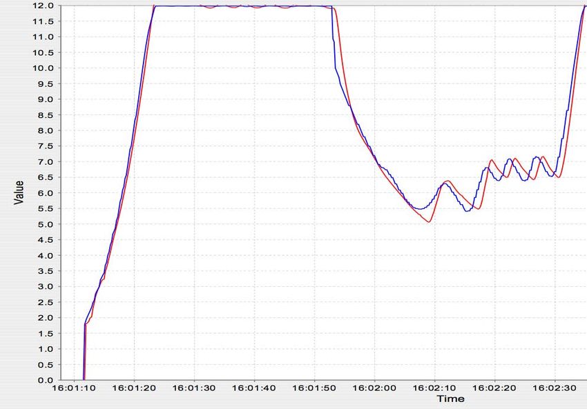
Figure 1: Team Gray’s Kat-5 as entered in the 2005 Grand Challenge.

rocks, boulders, fences, and other natural or man-made obstacles [DARPA, 2005b]. The route to
be followed was unknown by the team until two hours before the start of the race. It consisted
of a series of GPS waypoints which were an average of 275 feet apart. For each waypoint, an
acceptable lateral boundary around the waypoint was also specified. The sequence of waypoints
and the lateral boundaries specified a corridor that the vehicle had to stay within or the vehicle
could be disqualified by officials (see Figure 2). The route was only given as a sequence of GPS
waypoints but otherwise it was completely unknown; not just unrehearsed. The rules did not
prevent normalization of DARPA’s data before they were fed to the vehicles, neither did they
prevent elevation map databases, however, Kat-5 did not make use of any information other than
its sensor readings and DARPA’s waypoint data given to it in raw form.

              Figure 2: The corridor as defined by DARPA. See [DARPA, 2005a].

These conditions presented many challenges that needed to be met by innovative hardware and
software design. The following subsections present an overview of each of the main challenges
provided by the DARPA Grand Challenge.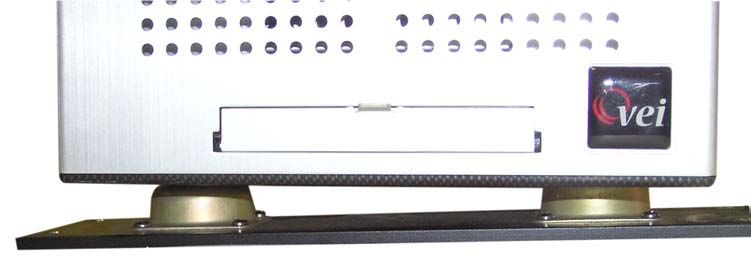
2.1   Endurance and Reliability

The actual race route was a substantial distance of 132 miles which had to be completed without
refueling or pit stops. Having to endure this length of distance in rough terrain at relatively high
speed is a massive endurance test for any vehicle, let alone a vehicle operating autonomously.
Every piece of hardware on the vehicle could become a failure point due to the excessive shock
and vibration caused by the rough terrain.

2.2   Environment Sensing

All decision making for steering and other controls had to be based solely on the data collected by
the vehicle’s onboard sensors. This introduces a major problem as collecting and fusing sensor data
can be a computationally expensive process and the sensor data itself can be difficult to interpret
[Coombs et al., 2001]. In addition, the vehicle must be able to accurately identify its own position
through an onboard sensor. The data readings then have to be coordinated with position readings.
Timestamping is complicated by delays of the onboard computer networks.

2.3   Artificial Intelligence

Based solely on the sensory data collected, the vehicle needed to independently decide how to
generate control signal sequences for steering, braking, and acceleration so that it could avoid
obstacles and stay within the given course. In addition, it needed to adjust speed to make sure that
the vehicle would execute turns safely.

2.4   Control Systems

The combination of all of the aforementioned navigational constraints along with the requirement
for high vehicle speed created the need for a very agile set of physical actuators and control algo-
rithms. These algorithms and actuators had to respond to the need for abrupt changes in speed and
steering quickly in order to handle the rapidly changing environment.

In addition to the above, this team had to work on a short development timeline. Unlike many
of the other teams that competed in the 2005 Grand Challenge, this team entered the competition
at a late date. As a result, we effectively had only six months to create and test the complete
autonomous vehicle.

3     System Design

A 2005 Ford Escape Hybrid was used as the base vehicle platform for the autonomous vehicle. This
vehicle contains both a typical four-cylinder gas engine and a 330-volt electric motor/generator.
The hybrid system allows for the vehicle to adapt intelligently to many different driving situa-
tions with maximum efficiency and performance by automatically using a combination of the two.
[Ford Motor Company, 2005]. This ensures maximum fuel economy, but still acceptable perfor-
mance. This vehicle was chosen because of the system that it was already outfitted with in order
to power its electric motor. This system was capable of supplying enough clean power for the
additional onboard electronics without an additional alternator or generator. It also had sufficient
ground clearance for rough terrain and a wheel base that offered a good balance between agile
maneuverability and stability.

During this project, the physical vehicle was viewed as a ”black-box” and was only interfaced with
at the highest level. The following sections describe the hardware components that were used to
make the vehicle capable of operating autonomously and handling the challenges presented in the
previous section. The hardware architecture for Kat-5 is outlined in Figure 3.

                       Figure 3: The communication architecture in Kat-5.

3.1   Computing Devices

The computing capacity for the autonomous vehicle was provided by a computing grid consisting
of four networked computers. The computers included two identical marine computers running
Linux and two identical Apple Mac Mini computers running OS X. Marine computers (made for
use on boats) were used as the two main computers because they would run on 12 volts of direct
current without modifications to their power supplies and also because they already had integrated
shock mounts. One of the marine computers was dedicated to processing data from the sensors,
while the other was dedicated to producing navigation control signals. The Mac Mini performed
all of the path planning.

A key challenge associated with the computing devices was making them hardened against shock
and vibration. The two marine computers were designed for a hostile environment, so they came
with integrated shock mounts and were capable of withstanding shocks of up to 30 Gs. Also,
each of their connections (both internal and external) came reinforced with silicon glue and other
restraints to ensure that they could not come loose due to shocks and vibrations encountered in
rough seas. A similar shock mount system was also created in house for the Mac Minis. An image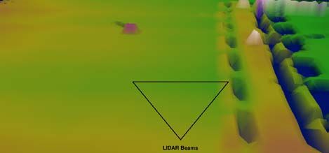
of the shock mount system is shown in Figure 4. The computing devices were linked together
by a rugged Cisco 2955 Catalyst switch capable of handling shocks of up to 50 Gs. A mix of
UDP and TCP protocols were used for the ethernet communications, with UDP being used for
communications where reliability was not as important as speed and TCP for communications
where reliability was paramount.

Figure 4: The shock mount system for the navigation computer could withstand shocks of up to 30
Gs.

3.2    Vehicle Actuators

Interfacing with the primary vehicle controls (steering wheel, accelerator, and brake) was accom-
plished by a custom drive-by-wire system designed by Electronic Mobility Controls (EMC). This
is a custom solution designed to outfit vehicles for handicapped drivers. It consists of actuators and
servos mounted on the steering column, brake pedal, throttle wire, and automatic transmission. It
is primarily controlled by a console with a touch-sensitive screen and an evaluator’s console which
contains a throttle/brake lever and a miniature steering wheel. We bypassed these controls and
connected the equipment’s wire harness to a computer via a digital to analog board. Thus, the
electrical signals that the manual controls would normally produce were actually produced by the
computer (which later will be referred to as the navigation computer). These electrical signals took
the form of the analog voltages shown in Table 1.

      Input                Voltage Range   Digital Steps Software Range
      Steering             0.4V to 4.6V        512       -250 (left lock) to 250 (right lock)
      Accelerator/Brake    0.4V to 4.6V        256       -124 (full brake) to 124 (full accel-
                                                         erator)
 Table 1: Input voltages and corresponding digital ranges for interfacing with EMC equipment.

The EMC equipment was chosen because it inherently satisfied many of the previously mentioned
challenges. Since the equipment is designed for handicapped drivers and must meet Department of
Transportation standards, it is fully redundant and very rugged. It also has a very fast reaction time
when given a command, so it can quickly turn the steering wheel or apply the brake if it needs to.
It was also able to be installed and tested very quickly by trained experts, so our short development
timeline was not adversely affected.

After initial testing during a hot summer day, we noticed that the computing equipment was over-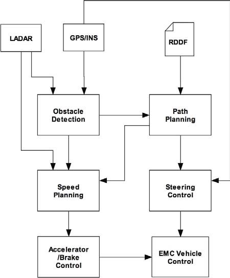
heating and then malfunctioning due to the high temperatures in the cabin of the car. This revealed
an issue between having proper fuel efficiency and having an acceptable cabin temperature. If the
air conditioner was kept on its highest setting, the equipment did not overheat, but the resulting
fuel economy was projected to be too low to finish the expected 175 mile race (projections were
based on the fuel economy of the 2005 Ford Escape 4 cylinder model). This lowered fuel econ-
omy was due to the fact that if the air conditoning system on a Ford Escape Hybrid is set to its
maximum setting, then the compressor must run constantly, which causes the gasoline engine to
also run constantly. This defeats the whole fuel efficient design of the hybrid’s engine as explained
previously.

As a result of this problem, we created a simple on/off mechanism for the air conditioning system
that was suited to the cooling needs of the equipment rather than the passenger’s comfort. The
device consisted of a temperature sensor, a BASIC stamp, and a servo motor. We mounted the servo
to the air conditioning system’s control knob so that the servo could turn the air conditioner on and
off. The BASIC stamp is a simple programmable micro-controller with 8 bidirectional input and
output lines and a limited amount of memory which can hold a small program. We programmed
the BASIC stamp to monitor the temperature of the cabin near the equipment. If the temperature
dropped below a certain threshold, the air conditioner was turned off. If the temperature rose above
a certain temperature, the air conditioning system was turned to its maximum setting. This simple
system solved our temperature problems while not adversely affecting our fuel efficiency, yet still
only interfacing with the vehicle at its highest level.

3.3   Positioning System

The position and pose of the car is reported by an Oxford Technical Solutions RT3000, an in-
tegrated Global Positioning System (GPS) with two antennas and an Inertial Navigation System
(INS). This system ensures that the vehicle is aware of its position on the Earth with a best-case
accuracy of less than 10 centimeters. This accuracy is possible due to its use of the Omnistar
High Performance (HP) GPS correction system. Nominal accuracies of the different parameters
available from the RT3000 are shown in Table (2).
                                 Parameter              Accuracy
                                 Position                10 cm
                                 Forward Velocity      0.07 km/hr
                                 Acceleration            0.01 %
                                 Roll/Pitch           0.03 degrees
                                 Heading              0.1 degrees
                                 Lateral Velocity         0.2 %
Table 2:      Accuracies of primary           vehicle    parameters    given    by   the    RT3000.
[Oxford Technical Solutions, 2004]

The RT3000 uses a Kalman filter to blend all of its inputs so as to derive clean unbiased estimates
of its state. A Kalman filter is a method of estimating the state of a system based upon recursive
measurement of noisy data. In this instance, the Kalman filter is able to much more accurately
estimate vehicle position by taking into account the type of noise inherent in each type of sensor
and then constructing an optimal estimate of the actual position [Kelly, 1994]. In the standard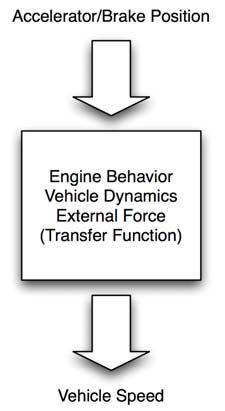
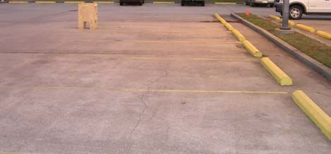
RT3000, there are two sensors (GPS and INS). These two sensors complement each other nicely
as they both have reciprocal errors (GPS position measurements tend to be noisy with finite drift
while INS position measurements tend to not be noisy but have infinite drift) [Bruch et al., 2002].

The RT3000 also accepts additional custom inputs to reduce drift in its estimate of vehicle position
when GPS is not available. This is important since when GPS is not present, the estimate of
position will begin to drift due to the Kalman filter’s heavy reliance on INS measurements. One
of these custom inputs is a wheel speed sensor which provides TTL pulses based upon an encoder
placed on a single wheel on the vehicle. When a wheel speed sensor is added to the RT3000,
it initially uses GPS data to learn how these TTL pulses correspond to actual vehicle movement.
Then when GPS data is not available due to tunnels, canyons, or other obstructions, the RT3000 is
able to minimize the positional drift by making use of the wheel speed sensor and its latest reliably
known correspondence to the vehicle’s movement. [Oxford Technical Solutions, 2004].

The wheel speed sensor consisted of a digital sensor capable of detecting either ferrous metal or
magnets that are in motion. We mounted it in the wheel well adjacent to the stock Antilock Brake
System (ABS) sensor, which allowed the wheel speed sensor to read the same magnets mounted
on the wheel that the ABS sensor did.

This level of accuracy allowed the car to precisely know its location on the earth, and therefore
made the artificial intelligence algorithms much more accurate. Its 100 Hz refresh rate also notified
the control systems of positional error very quickly, which allowed for immediate corrections in
course due to bumps from rough terrain and other sources of error.

3.4   Vision Sensors

Two Sick LMS 291 Laser Detecting and Ranging (LADAR) devices provided the autonomous
vehicle with environmental sensing. Each LADAR device scans a two-dimensional plane using a
single pulsed laser beam that is deflected by an internal rotating mirror so that a fan shaped scan
is made of the surrounding area at half-degree intervals [Sick AG, 2003]. Rather than pointing the
LADAR devices at the ground horizontally, we mounted the LADAR devices vertically. We chose
to align them vertically because it made obstacle detection much easier. In the simplest case, by
analyzing the measurement data beam by beam in angular order, obstacles were easy to locate as
either clusters of similar distance or gaps in distance [Coombs et al., 2001].

A set of two 12 volt DC batteries connected in series supplied the required 24 volts of DC current
required for the two Sick LADAR devices. These two batteries were then charged by an array
of six solar panels that were placed on the top of the vehicle’s aluminum rack. These solar pan-
els were then divided into two sets of three panels each, and each set was connected to a solar
regulator which monitored the status of the corresponding battery that it was connected to, and
provided charge when necessary. The solar panels were the only source of power supplied to the
two batteries that comprised the 24 volt power system.

Next, we built a platform that oscillated back and forth, so that the LADAR units would scan all
of the terrain in front of the vehicle repeatedly. To ensure that we knew the precise angle at which
the LADAR devices were pointed at any time, an ethernet optical encoder from Fraba Posital was
placed on the shaft which was the center of rotation. The optical encoder provided both the current
angle and the angular velocity of the shaft. To decrease the delay between reading a value from the
sensor and reading a value from the encoder, a separate 100 MBit ethernet connection with its own
dedicated ethernet card was used to connect the I/O computer with the encoder. This delay was
assumed to be the result of the TCP protocol’s flow control algorithms [Jacobson and Karels, 1988]
and their handling of congestion in the ethernet switch. After placing each encoder on its own
dedicated ethernet connection, communications delays between the encoder and the I/O computer
were relatively consistent at approximately .5 ms.

Testing revealed that the actual LADAR scan was taken approximately 12.5 ms before the data was
available at the I/O computer. When this time was added to the .5 ms of delay from the encoder
communications, we had a 13 ms delay from the actual scan to the actual reading of the encoder
position and velocity. To counteract the angular offset this delay created, we multiplied the velocity
of the encoder times the communications delay of .013 seconds to calculate the angular offset due
to the delay. This angular offset (which was either negative or positive depending on the direction
of oscillation) was then added to the encoder’s position, giving us the actual angle at the time when
the scan occurred. This extra processing allowed us to accurately monitor the orientation of the
LADAR platform to within .05 degrees.

Although the vehicle’s vision system was only comprised of these two LADAR devices, their
oscillating platforms and vertical orientation allowed them to sense the environment with very fine
detail and as precise an accuracy as possible. Figure 5 shows an actual picture of a parking lot and
the resulting maps from the sensor readings. Several holes are visible in the 3D elevation map,
especially along the right side of the image. These are artifacts created by the fact that the lasers
cannot see behind obstacles. Therefore, the section behind an obstacle will have no elevation data
associated with it. We designed both oscillating mounts to cover a thirty degree range and mounted
each of them on different sides of the vehicle. This allowed us to have much finer detail in the
center of the path, as both LADAR devices were able to scan this area. It also offered redundant
coverage in the center of the path so that if one sensor failed, the vehicle could still sense obstacles
most likely to be directly in its path.

Figure 5: A sample 3D elevation map (a) created by the vision system and the actual terrain (b) it
was created from.
All sensor readings had to be converted to a common coordinate system, which was chosen to
be the geospatial coordinate system because the GPS reports vehicle position in the geospatial
coordinate system. The two Sick LMS 291 LADAR units captured a two-dimensional scan of the
terrain in front of the vehicle along with the exact time at which the scan took place. Using the
highly accurate data from the RT3000, these two-dimensional scans were then transformed into
the vehicles coordinate frame and then into a geospatial coordinate frame via a set of coordinate
transformation matrices. This is accomplished in two similar steps. In each step a transformation
matrix is defined so that
P2 = T1→2 P1 + ∆1 (1)
where T1→2 is the transformation matrix for going from coordinate frame 1 to coordinate frame
2, ∆1 is the vector representing the position of the origin of coordinate frame 1 with respect to
the origin of coordinate frame 2, and P1 and P2 are the same point in coordinate frames 1 and 2,
respectively.
The first step converts from the sensor coordinate frame to the vehicle’s coordinate frame. The
vehicle’s coordinate frame is located on the center of the rear axle of the vehicle and has the
standard X (longitudinal), Y (lateral) , and Z (vertical) axes orientation. The sensor’s coordinate
system is centered on the sensor with the sensor’s native X, Y, and Z axes. Therefore, the vehicle’s
coordinate system is related to the sensor’s coordinate system via rotations and translation. Thus,
a simple linear transformation of the form (1) can convert one to the other. This transformation is
defined through a matrix, Ts→v (to be used in place of T1→2 in Equation (1) ), which is defined as
cos ψs − sin ψs 0 cos θs 0 sin θs 1 0 0
Ts→v sin ψs
= cos ψs 0 0 1 0 0 cos φs − sin φs (2)
0 0 1 − sin θs 0 cos θs 0 sin φs cos φs
where ψs , θs , and φs are the yaw (around the z-axis), pitch (around the y-axis), and roll (around the
x-axis) of the sensor coordinate frame relative to the vehicle’s coordinate frame. This transforma-
tion takes into account deviations in yaw, pitch, or roll caused by the mounting of the sensor. For
example, if the sensor were mounted pointed slightly downward, it would have a negative pitch
that would need to be countered by setting θs to its inverse (or positive) value. In addition, the
angle of deflection caused by the oscillation is processed here by adding it to φs .
The same basic transformation and translation was done again in order to translate from the vehi-
cle’s coordinate system to the common geospatial coordinate system. Yet another transformation
matrix, Tv→g , was constructed for this purpose.
cos ψv − sin ψv 0 cos θv 0 sin θv 1 0 0
Tv→g sin ψv
= cos ψv 0 0 1 0 0 cos φv − sin φv (3)
0 0 1 − sin θv 0 cos θv 0 sin φv cos φv
where ψv , θv , and φv are the heading (around the z-axis), pitch (around the y-axis), and roll (around
the x-axis) of the vehicle relative to the geospatial coordinate system. These heading, pitch, and
roll values are generated by the GPS/INS navigation sensor that is mounted on the vehicle.
After taking into account both of these transformation matrices, the full equation for transformation
from sensor coordinate system to geospatial coordinate system isPg = Tv→g (Ts→v Ps + ∆s ) + ∆v . (4) where ∆s is the vector representing the position of the sensor with respect to the center of the vehicle and ∆v is the vector representing the position of the center of the vehicle with respect to the center of the GPS/INS navigation sensor. At this point, each of the measurement values from the LADAR units now has a latitude, longitude, elevation, and timestamp. These elevation values are then placed into the same elevation grid, where the number of scans and time since last scan are used to derive the probability that the vehicle can drive over that geospatial location. We now describe how this probability is derived. The data from the two sensors are correlated by placing data from both sensors into the same elevation grid (see Figure 5 for an example of this). The routines that this team developed to build internal representations for maps do not need to account for which sensor saw the obstacle, but only the number of times any sensor saw the obstacle and how recently did a sensor see the obstacle. As a result of this, any number of LADAR sensors can be used without having to change the algorithms at all. The timestamp is very important to the algorithms due to the fact that LADAR scan data can have anomalies in it. Highly reflective surfaces can cause the LADAR devices to register incorrect distances for obstacles. To counteract these anomalies, scans are only kept in memory for a certain amount of time. After that time has passed, if no more obstacles have been registered in that same area, the obstacle is removed. This also ensures that moving obstacles are handled correctly. If a vehicle or other object crossed the path perpendicular to the autonomous vehicle, the sensors would effectively register a sequence of obstacles in front of the autonomous vehicle. These obstacles would appear as a complete obstruction of the vehicle’s path, forcing the vehicle to immediately stop. After enough time had passed, the obstacles would expire, and the autonomous vehicle would be able to start moving again. A persistent obstacle, on the other hand, will not expire. Consider, for example, a large boulder that is located in the center of the path. At a distance of approximately forty to fifty meters, the LADAR devices will start to register parts of the boulder. As the autonomous vehicle gets to within ten to twenty meters of the vehicle, the previous scans would begin to approach the obstacle expiration time. Since the sensors are still registering the boulder, the previous scans will not expire. Instead, the previous scans along with the current scans would all be retained, giving the boulder a higher count for total number of scans. This high count for the number of scans causes the boulder to have an extremely high probability of being an obstacle. 4 Software Design Software played a critical role in the design of the autonomous vehicle. Rather than using the C programming language to build the software for Kat-5 like virtually all of the other teams compet- ing in the DARPA Grand Challenge, we decided to use the Java programming language instead. While many detractors might say that Java offers slower performance and lacks conventional par- allel programming models [Bull et al., 2001], we decided that its benefits outweighed its deficien-
cies.

It was imperative in the design of Kat-5 that all systems, physical or software, be completely mod-
ular and independent of platform or peers. This requirement was met fully from the beginning
of development within the software realm by the use of the Java programming language. Java’s
simple language semantics, platform independence, strong type checking, and support for con-
currency have made it a logical choice for a high integrity system [Kwon et al., 2003] such as an
autonomous vehicle.

Because of the platform-independance of Java, we were able to use multiple hardware solutions
that fit different niches in our overall design. All of the interface systems were deployed on Linux
systems while the math-intensive processing was performed primarily on Apple systems. Despite
this disparity in operating systems, all computers were given the same exact executables. A block
diagram of our process architecture is shown in Figure 6.

Figure 6: The software used in driving the vehicle is a highly modular system
[Trepagnier et al., 2005].

To ensure the quality of our code base, we followed the practices of Test Driven Development
which is a software development practice in which unit test cases are incrementally written prior
to code implementation [George and Williams, 2003]. As a result of this, we created unit tests for
all critical software modules on the vehicle. This allowed us to run the unit tests each time we
deployed our code to detect if we had introduced any bugs. This alone saved us enormous amounts
of time and helped to provide us with the stable code base that allowed us to finish the Grand
Challenge.

For example, geospatial operations such as projecting a point a given distance along a heading
(or bearing) or converting between different coordinate systems were some of the most commonly
used pieces of code on the vehicle. These geospatial operations were also consistently modified
and improved throughout development. To ensure that this ongoing development did not introduce
errors into this critical part of the code base, unit tests were created to test each geospatial operation.
These unit tests were created by performing the operations manually, then using these results to
craft a unit test that ensured that the given operation produced the same results. Each geospatial
operation had several of these tests to ensure complete testing coverage of each operation.

The following subsections describe our use of Java to develop the software necessary to meet the
challenges described in the previous section.

4.1   Path Planning and Obstacle Avoidance

Path Planning is accomplished through the use of cubic b-splines [de Boor, 1978] designed to
follow the center of the route while still ensuring that the path they create is not impossible for the
vehicle to navigate. This assurance means that the curvature at any point along the path is below
the maximum curvature that the vehicle can succesfully follow. In addition, the curvature is kept
continuous so that it is not necessary to stop the vehicle in order to turn the steering wheel to a new
position before continuing.

B-splines were chosen for use in the path planning algorithms primarily because of the ease in
which the shape of their resulting curves can be controlled [Berglund et al., 2003].After an initial
path is created that follows the center of the corridor, the path is checked against the obstacle
repository to determine if it is a safe path. If the path is not safe, a simple algorithm generates and
adjusts control points on the problem spots of the curve until the spline avoids all known obstacles
while still containing valid maximum curvature. At this point, the path is both safe and drivable.

Once a safe path is designed that avoids obstacles and yet remains drivable, the next step in the
planning process is to decide on the speed at which the vehicle should take each section of the
path. The speed chosen is based on the curvature at that point in the path and upon the curvature
further down the path. The speed is taken as the minimum of speed for the current curvature and
the speed for future path curvature. The future path curvature is defined by a simple function that
multiplies the curvature at a given future point by a fractional value that decreases towards zero
linearly based upon the distance from the current path point to the given future path point.

4.2   Speed Controller

In order to design intelligent controls suitable for a given system, that system, in this case the car’s
engine and the external forces, must be understood. System identification is a method by which
the parameters that define a system can be determined by relating input signal into a system with
the system’s response [Aström and Wittenmark, 1995]. It is the goal of this method to develop a
transfer function that behaves in the same way as the actual system. For instance, when attempting
to control the speed of a vehicle, the inputs are the brake and accelerator position and the output is
the vehicle’s speed (see Figure 7). If it is assumed that the transfer function, H(s), is first-order, it
can be written as
Figure 7: The transfer function developed through system identification is intended to characterize
the reaction of the system to the inputs.

                                           y(s) = H(s)u(s)                                          (5)

where H(s) is the transfer function of a system, u(s) is the input to the system, and y(s) is the
output from the system. System identification, as described in [Aström and Wittenmark, 1995],
was applied to real world data from the propulsion system to come up with the transfer function of
the system.

As far as the speed control of the vehicle was concerned, it seemed like a simple control system
could be designed to handle the accelerator and brake. However, as it turned out, there were many
factors in the physical engine system that made for a fairly complex transfer function. Being a gas-
electric hybrid engine, the coupling of the two propulsion systems was controlled by an intelligent
computer tuned for fuel efficiency, a computer that we had no information about. In addition, the
mapping of the requested pedal position and the actual position achieved was not linear and had to
be remapped in the software layer.

It was eventually decided that the speed of the vehicle would be controlled by an integrated
proportional-derivative (PD) controller [Aström and Wittenmark, 1995]. This controller bases its
output on the previous output and on the current error and derivative of the error. In the time
domain, the controller can be written as

                           u(t2 ) = (t2 − t1 )(Kp e(t2 ) + Kd e0 (t2 )) + u(t1 )                    (6)

where Kp and Kd are tunable coefficients, u(t) i the output of the controller at time t, and e(t) is the
error at time t. The error is defined in a conventional manner: actual output subtracted from target
output. Actual output is reported by the RT3000 and target speed is derived from the path planning
algorithms. Since the actual output is limited to u(t) ∈ [−1, 1], no windup of the controller is
experienced. There was some overshoot and oscillation inherent in the system but with tuning it
was reduced to a manageable level (see Figure 8).
The integrated PD controller was designed and tuned against the transfer function that we had
arrived at through the system identification process mentioned above. It was a simple matter to
arrive at the weights needed for optimal performance against the computational model; however,
the computational model was a far cry from the true real-world system. The modeled values were
used as a baseline from which to work from when tuning the real controller.
Figure 8: The PID comes very close to matching current speed to target speed during a run at the
NQE.
4.3 Steering Controller
The steering controller for the vehicle was a lead-lag controller based on the classical single-track
model or bicycle model developed by Riekert and Schunck [Riekert and Schunck, 1940].
The transfer function from steering angle to vehicle lateral acceleration may be written as
µcf v 2 (M lf ds + IΨ ) s2 + µ2 cf cr lv (ds + lr ) s + µ2 cf cr lv 2
(7)
IΨ M v 2 s2 + µv IΨ (cf + cr ) + M cf lf2 + cr lr2 s + µM v 2 (cr lr − cf lf ) + µcf cr l2
The introduced variables are defined in Table 3.
By applying the Laplace integrator twice we obtain the transfer function from steering angle df (s)
to the lateral displacement yS (s).Symbol Description
M Vehicle mass
v Vehicle velocity
ψ Vehicle yaw with respect to a fixed inertial coordinate system
Iψ Yaw moment of inertia about vertical axis at CG
lf /r Distance of front/rear axle from CG
l lf + lr
yS Minimum distance from the virtual sensor to the reference path
df Front wheel steering angle
dS Distance from virtual sensor location to CG
cf /r Front/rear tire cornering stiffness
µ Road adhesion factor
Table 3: Variables used in the steering controller’s vehicle model.
The state space representation as found in [Hingwe, 1997] may be written as
ẋ = Ax + Bu (8)
where
ys
ẏs
x = u = δf (9)
Ψ
Ψ̇
and
0 1 0
0
φ1 (dS − lf ) + φ2 (dS + lr )
(φ1 + φ2 )
0
− v
φ1 + φ2 v
A = (10)
0 0 0 1
(cf (lf2 − lf dS ) + cr (lr2 − lr dS ))
(lf cf − lr cr ) (lf cf − lr cr )
0 − 2 −2
IΨ v
2 IΨ IΨ v
0 0
(φ2 lr − φ1 lf − v2 )
B =
φ1 v
(11)
0 0
where
!
1 lf dS
φ1 = 2cf + (12)
M IΨ!
1 lr dS
φ2 = 2cr + (13)
M IΨ
The outputs of the vehicle model as shown in Equation 14 are the lateral error at the virtual sensor
and the yaw.
h i
y = 1 0 dS 0 x (14)
Lead and lag compensators are commonly used in control systems. A lead compensator can in-
crease the responsiveness of a system; a lag compensator can reduce (but not eliminate) the steady
state error [Bernstein, 1997]. The lead-lag compensator was designed using the frequency response
of the system. The lead compensator used is stated in (16) and the lag compensator is stated in
(15). The resulting controller is the convolution of the two functions multiplied by the low fre-
quency gain, which was 0.045. The parameters used in (16) and (15) were produced using rough
estimates which were then tuned by trial and error.
850s + 1
Flag (s) = (15)
900s + 1
2s + 4
Flead (s) = (16)
0.2s + 1
The step response of the closed-loop system is shown in Figure 9.
The input to the controller is defined as [yS ] where yS refers to the minimum distance from the
virtual sensor to the reference path. The virtual sensor is a point projected a given distance ahead
of the vehicle along the vehicle’s centerline. This point is commonly referred to as the look-ahead
point, and the distance from the look-ahead point to the RT3000 is referred to as the look-ahead
distance. The output of the controller is the steering angle measured at the tire with respect to the
centerline.
Control gains were not scheduled to the speed of the vehicle. Gain scheduling was evaluated,
but not implemented, as the steering controller by itself offered more than enough stability and
accuracy. No additional knowledge, such as whether the vehicle was going straight or in a turn,
was given to the steering controller.
Several assumptions were made in implementing this model. The relationship between the steering
wheel angle and the resulting tire angle was assumed to be linear. The measurements made of this
relationship showed that the actual variation was negligible. Also, the location of the vehicle’s
center of gravity was assumed to be at the midway point between the front and rear axles.
The steering controller managed to provide incredible accuracy, even at speeds of over thirty miles
per hour. An analysis was made of the steering controller’s accuracy from the first 28 miles of the
2005 DARPA Grand Challenge. An unfortunate error that is described later in Section V preventedFigure 9: Step response of closed-loop system. the team from being able to perform an analysis on more data from the Grand Challenge. As shown in Figure 10, the steering controller was able to maintain a standard deviation of 5 centimeters in regards to the desired path. This is an excellent performance, especially when considering the roughness of the terrain and a top speed of over 35 mph for Kat-5. As a measure of safety the magnitude of the ys signal was monitored to prevent the vehicle from becoming unstable. If ys were ever to cross a given threshold, meaning the vehicle is severely off path, the speed was instantly reduced to 2 mph. This allowed the vehicle to return onto the desired path and prevented a possible rollover. The algorithm was repeatedly tested by manually overriding the steering controller and taking the vehicle off path, then allowing it to regain control. This algorithm proved to be very effective. Figure 10 shows the path error from the first 28 miles of the 2005 Grand Challenge, and a 1.5 meter spike at around the 2000 second mark. At this point, a GPS jump caused a spike in path error from 5 cm to 1.5 meters in a span of just 10 ms. As shown in Figure 11, the steering controller was able to handle this GPS jump safely and quickly, and return Kat-5 back to the proper planned path. 5 Field Testing Initial field testing concentrated on improving the accuracy of both the speed controller and steering controller at low to medium speeds. After extensive testing at these speeds, the team rented out a local racetrack, and proceeded to ensure that the vehicle could operate reliably at higher speeds. Throughout this entire process, both the speed controller and steering controller were progressively
Figure 10: The steering controller proved to have an extremely high accuracy during the 2005
DARPA Grand Challenge. The standard deviation for the 28 miles shown here was just 5 cm from
the desired path.

tuned, until they both operated with the accuracy required for the Grand Challenge. During these
tests, the accuracy of the steering controller was able to be increased from over 50 cm to less than
5 cm.

Before taking the vehicle to California for the Grand Challenge National Qualification Event
(NQE), the vehicle was put through several strenuous tests designed to test not only hardware
and software endurance and reliability, but also vehicle performance. Throughout this testing, the
vehicle was subjected to harsh terrain, difficult obstacle avoidance scenarios, and long run times.
Unfortunately, due to weather-related circumstances outside of our control (Hurricane Katrina),
the amount of time available for final testing of Kat-5 was severely limited.

The NQE was used by DARPA to pare down the 43 semifinalists to a pool of 23 finalists. At the
National Qualification Event which was held at the California Motor Speedway in Los Angeles,
California, Kat-5 ran into several problems initially which were the result of a lack of thorough
testing before the event. Several quick changes were made to the software and hardware, which
allowed Kat-5 to produce several successful runs at the end of the NQE and advance to the Grand
Challenge Event. The results of Kat-5’s seven qualifying runs are listed below:

Run 1 – Did Not Finish
      At the end of the fast portion of the course, Kat-5’s geospatial system encountered a failed
      assertion in its geospatial processing algorithm and shut down. Without a course to follow,
      the vehicle continued straight ahead, missing a right turn and hit the side-wall at approxi-
Figure 11: The steering controller handled this GPS jump by reducing speed to allow the vehicle
to safely steer back onto the planned path.
mately 20 miles per hour (8.94 m/s) causing some damage to the front body, but no major
structural damage. The assertion was caused by a bug in the code that created a composite
polygon from the individual polygonal segments of the corridor. Apparently, the composite
polygon created in one section of the NQE course was not a valid polygon, and this caused
a failed assertion error. To get around this bug, the algorithm was changed to use the in-
dividual segments directly rather than the composite polygon composed of the individual
segment polygons.
Run 2 – Did Not Finish
The GPS position of the vehicle was reported as two to three meters north of its true loca-
tion. While attempting to enter the tunnel, the vehicle saw the entrance, but thought that
the entrance was off of the course, and thus it could not navigate so as to enter the tunnel
without going out of bounds. The front left of the vehicle hit the corner of the entrance.
Major damage was done to the front end, but it was repaired quickly. The RT3000 has a
basic GPS component but it is also using a ground OmniStar Correction Service to further
refine the readings of the GPS component and thus provide finer accuracy than is possible
on GPS alone. Upon investigation, it was discovered that the ground station frequency used
by the RT3000 for OmniStar Correction Service was still set to the one corresponding to
the eastern United States rather than the western United States and thus during the previous
runs only basic GPS was actually used.
Run 3 – Did Not Finish
After approximately 100 meters, the circuit breaker in the engine compartment of the ve-
hicle overheated and popped open, cutting power to all of the vehicle’s robotic systems.The drive-by-wire system used its reserve power to apply the brake and then shut off the
vehicle. The circuit breaker was replaced with a heavy-duty wire and locking disconnect
plug.
Run 4 – Finished in 16:42
Kat-5 completed the entire 2.2-mile course. Upon exiting the tunnel, the vehicle gunned its
accelerator causing it to leave the corridor before slamming on its brakes. After reacquiring
a GPS lock, it navigated back onto course and continued to the end where it finished the
course.
Run 5 – Finished in 15:17
Kat-5 had a perfect qualifying run until the very end of the course where it completely
failed to avoid the tank trap. It hit the obstacle, but continued its forward motion, pushing
the tank trap across the finish line. Data analysis indicated that the position of the sun on
the extremely reflective tank trap caused both LADAR devices to be blinded.
Run 6 – Did Not Finish
Upon exiting the tunnel, the vehicle behaved as it did in run 4, but when it recovered GPS
lock, it began driving in circles. It had to be shut down remotely. There was a logical error
in one of our recovery systems that did not allow the vehicle to draw a path back onto the
course after recovering from failure in the RT3000. There were several bugs in the RT3000
itself that caused its integrated INS to lag almost five full seconds behind its integrated
GPS. Although the RT3000 is designed to handle GPS outages with little performance
degradation in normal working conditions, these bugs created significant problems that
caused a drift of over 5 meters when GPS signal was lost. After an hour of work on-site
with engineers from Oxford Technical Solutions, the problems were quickly diagnosed
and fixed, then incorporated into an upgraded firmware release for the RT3000 by Oxford
Technical Solutions.
Run 7 – Finished in 15:21
Kat-5 completed its first and only perfect run, securing its spot as a finalist.
Several images of the output of the path planning systems during actual runs from the NQE are
shown in Figures 12, 13, and 14. In this visualization, obstacles are represented by clusters of
points and the path is represented by the sparse sequence of dots.
The Grand Challenge was held on October 8 in Primm, Nevada. Kat-5 was one of the twenty-three
finalists that was able to participate in the race. She left the starting line with a burst of speed and
never looked back. Kat-5 finished the race in an elapsed time of seven hours and thirty minutes
with an average speed of 17.5 mph to claim fourth place. Several issues were discovered after
analyzing the vehicle during a post-race inspection.
• The vehicle’s steering was severely out of alignment. The team assumed this was due
to Kat-5’s attack of the rough terrain at relatively high speed. Amazingly, the steering
algorithm was able to easily handle this issue, as evidenced by the fact that Kat-5 was able
to complete the race.
• The Antilock Braking System was displaying intermittent failures that caused the brakes
to behave in an erratic fashion. This issue was also assumed to be the result of the roughFigure 12: Kat-5 is planning a path to avoid an obstacle in the center of the path at NQE. The
vehicle is moving towards the top right.
terrain. Like the steering controller’s ability to handle the problem steering alignment , the
speed controller also was able to handle the erratic brakes.
• The logging system crashed after 28 miles. This unfortunate issue means that a full analysis
of the Grand Challenge for Kat-5 is impossible. The cause for this crash was apparently a
crash of the logging server Java program running on the logging computer. The root cause
of this is currently undetermined, but the primary suspect is that diagnostic information
produced by the error discussed in the next item caused some piece of executing code to
throw an unchecked exception. This unchecked exception caused the Java Virtual Machine
to exit.
• The only major flaw in Kat-5’s performance on the day of the Grand Challenge was an
error in the path planning algorithms that caused them to time out when faced with sections
of the route with extremely wide lateral boundaries.
We had anticipated that the path planning algorithms might occasionally time out, and
therefore we had programmed Kat-5 to slow down to 3 mph for safety reasons until the
algorithms had a chance to recover. However, whenever Kat-5 encountered sections with
an extremely wide lateral boundary, the algorithms timed out continuously due to the error
until a section with a narrower lateral boundary was encountered. This caused Kat-5 to
drive the dry lake bed sections of the race, which were considered the easiest, at 3 mph
instead of 40 mph. Calculations by both DARPA and Team Gray about the time lost due
to this bug have shown that if this error had not occurred, Kat-5 would have posted a much
better finishing time. This bug has since been fixed.Figure 13: The path planning algorithms identified an obstacle at NQE and avoided it. The vehicle is moving towards the top right. 6 Conclusion The recipe of success in this effort was rugged hardware, simple software, and good teamwork. We chose to use off-the-shelf, proven hardware that we customized as needed. This allowed rapid development and also provided a reliable hardware platform that was not prone to failures. The harsh terrain could easily dislodge a wire or render a sensor or communications link useless and would therefore mean the end of the race. This was the motivation for choosing the EMC drive- by-wire system, the shock resistant equipment mounts, the rugged 50G tolerant Cisco equipment, and all of the other equipment. This was also the reasoning for choosing the RT3000 which not only was built to provide supreme accuracy but also was designed to take additional inputs from custom-made sensors and seamlessly incorporate them into its adaptive mechanism. The RT3000 produced better than 10 cm accuracy at an incredibly fast 100 Hz. As an off-the-shelf, industrial system, it is much more reliable than one that we would conceivably build ourselves. The simplicity of the design also resulted in an agile system. The sensor vision system of the vehicle was just two LADAR devices. All of the I/O bandwidth of the system was dedicated to reading just these two sensors. So the system was able to read massive data streams very quickly without much overhead for synchronization and fusion of the sensor streams. Thus, processing of the data was efficient and the computation of the control sequences was fast, resulting in a very agile overall system. While other sensors were considered for inclusion into the vision system, their contributions were not considered useful enough to warrant the complications they would
Figure 14: Kat-5 shows that she is capable of planning a path that can handle slaloming around
obstacles. The vehicle is moving towards the top left.

have added to the sensor fusion algorithms.

The choice of Java was also a good one since the development, monitoring, and testing were all
profoundly quick and produced code that was thoroughly validated before it even went into testing.
On another note, because of the portability of Java byte code, if we had to change our computing
grid architecture or even switch a PC with a Mac or add a new one of either platform to the overall
system it would not be any problem. The choices we made were well validated since the vehicle
endured the entire course well within the time limit and with only about 7 gallons of gas. We did
not win the race but participating in it was very rewarding as it validated our choices and methods.
Indeed, we like to think that reaching the finish line after 132 miles of autonomous driving in
the desert was not just beginner’s luck but rather the result of our simple design methods, good
decisions, and good system integration.

7   Acknowledgment

This project was entirely financed and supported by The Gray Insurance Company, Inc.

References
[Aström and Wittenmark, 1995] Aström, K. J. and Wittenmark, B. (1995). Adaptive Control. Ad-
  dison Wesley Lognman, Reading, Massachusetts, second edition.
[Berglund et al., 2003] Berglund, T., Jonsson, H., and Soderkvis, I. (2003). An obstacle-avoiding
  minimum variation b-spline problem. In 2003 International Conference on Geometric Modeling
  and Graphics (GMAG’03), page 156.
[Bernstein, 1997] Bernstein, D. (1997). A student’s guide to classical control. IEEE Control
  Systems Magazine, 17:96–100.
[Bruch et al., 2002] Bruch, M. H., Gilbreath, G., Muelhauser, J., and Lum, J. (July 9-11, 2002).
  Accurate waypoint navigation using non-differential gps. In AUVSI Unmanned Systems 2002.
[Bull et al., 2001] Bull, J. M., Smith, L. A., Pottage, L., and Freeman, R. (2001). Benchmarking
  java against c and fortran for scientific applications. In Java Grande, pages 97–105.
[Coombs et al., 2001] Coombs, D., Yoshimi, B., Tsai, T.-M., and Kent, E. (2001). Visualizing
  terrain and navigation data. Technical report, National Institute of Standards and Technology,
  Intelligent Systems Division.
[DARPA, 2005a] DARPA (2005a). 2005 darpa grand challenge rddf document.
[DARPA, 2005b] DARPA (2005b). 2005 darpa grand challenge rules.
[de Boor, 1978] de Boor, C. (1978). A practical guide to splines. Springer-Verlag.
[Ford Motor Company, 2005] Ford Motor Company (2005). Escape hybrid: How it works.
[George and Williams, 2003] George, B. and Williams, L. (2003). An initial investigation of test
   driven development in industry. In SAC ’03: Proceedings of the 2003 ACM symposium on
   Applied computing, pages 1135–1139, New York, NY, USA. ACM Press.
[Hingwe, 1997] Hingwe, P. (1997). Robustness and Performance Issues in the Lateral Control of
   Vehicles in Automated Highway Systems. Ph.D Dissertation, Dept. of Mechanical Engineering,
   Univ. of California, Berkeley.
[Jacobson and Karels, 1988] Jacobson, V. and Karels, M. J. (1988). Congestion avoidance and
   control. ACM Computer Communication Review; Proceedings of the Sigcomm ’88 Symposium
   in Stanford, CA, August, 1988, 18, 4:314–329.
[Kelly, 1994] Kelly, A. (1994). A 3d state space formulation of a navigation kalman filter for
  autonomous vehicles. Technical report, CMU Robotics Institute.
[Kwon et al., 2003] Kwon, J., Wellings, A., and King, S. (2003). Assessment of the java program-
  ming language for use in high integrity systems. SIGPLAN Not., 38(4):34–46.
[Oxford Technical Solutions, 2004] Oxford Technical Solutions (2004). RT3000 Inertial and GPS
  Measurement System.
[Riekert and Schunck, 1940] Riekert, P. and Schunck, T. (1940). Zur fahrmechanik des gum-
   mibereiften kraftfahrzeugs. In Ingenieur Archiv, volume 11, pages 210–224.
[Sick AG, 2003] Sick AG (2003). LMS 200 / LMS 211 / LMS 220 / LMS 221 / LMS 291 Laser
   Measurement Systems Technical Description.
[Trepagnier et al., 2005] Trepagnier, P. G., Kinney, P. M., Nagel, J. E., Dooner, M. T., and Pearce,
   J. S. (2005). Team Gray technical paper. Technical report, The Gray Insurance Company.
You can also read