Learning to Reconstruct Shape and Spatially-Varying Reflectance from a Single Image - UCSD CSE
←
→
Page content transcription
If your browser does not render page correctly, please read the page content below
Learning to Reconstruct Shape and Spatially-Varying Reflectance from
a Single Image
ZHENGQIN LI, University of California, San Diego
ZEXIANG XU, University of California, San Diego
RAVI RAMAMOORTHI, University of California, San Diego
KALYAN SUNKAVALLI, Adobe Research
MANMOHAN CHANDRAKER, University of California, San Diego
(a) (b) (c) (d) (e) (f ) (g) (h)
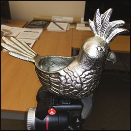
Fig. 1. We propose a novel physically-motivated cascaded CNN architecture for recovering arbitrary shape and spatially-varying BRDF from a single mobile
phone image. (a) Input image in unconstrained indoor environment with flash enabled. (b) Relighting output using estimated shape and SVBRDF. (c) Rendering
output in novel illumination. (d–g) Diffuse albedo, roughness, depth and surface normals estimated using our framework. (h) Normals estimated using a
single-stage network. Our cascade design leads to accurate outputs through global reasoning, iterative refinement and handling of global illumination.
Reconstructing shape and reflectance properties from images is a highly CCS Concepts: • Computing methodologies → Reflectance modeling;
under-constrained problem, and has previously been addressed by using 3D imaging; Shape inference; Reconstruction; Computational photography;
specialized hardware to capture calibrated data or by assuming known (or
Additional Key Words and Phrases: SVBRDF, single image, deep learning,
highly constrained) shape or reflectance. In contrast, we demonstrate that
we can recover non-Lambertian, spatially-varying BRDFs and complex ge- global illumination, cascade network, rendering layer
ometry belonging to any arbitrary shape class, from a single RGB image ACM Reference Format:
captured under a combination of unknown environment illumination and Zhengqin Li, Zexiang Xu, Ravi Ramamoorthi, Kalyan Sunkavalli, and Manmo-
flash lighting. We achieve this by training a deep neural network to regress han Chandraker. 2018. Learning to Reconstruct Shape and Spatially-Varying
shape and reflectance from the image. Our network is able to address this Reflectance from a Single Image. ACM Trans. Graph. 37, 6, Article 269 (No-
problem because of three novel contributions: first, we build a large-scale vember 2018), 11 pages. https://doi.org/10.1145/3197517.3201313
dataset of procedurally generated shapes and real-world complex SVBRDFs
that approximate real world appearance well. Second, single image inverse 1 INTRODUCTION
rendering requires reasoning at multiple scales, and we propose a cascade
network structure that allows this in a tractable manner. Finally, we incor-
Estimating the shape and reflectance properties of an object using
porate an in-network rendering layer that aids the reconstruction task by a single image acquired “in-the-wild” is a long-standing challenge
handling global illumination effects that are important for real-world scenes. in computer vision and graphics, with applications ranging from
Together, these contributions allow us to tackle the entire inverse rendering 3D design to image editing to augmented reality. But the inherent
problem in a holistic manner and produce state-of-the-art results on both ambiguity of the problem, whereby different combinations of shape,
synthetic and real data. material and illumination might result in similar appearances, poses
a significant hurdle. Consequently, early approaches have attempted
Authors’ addresses: Zhengqin Li, University of California, San Diego, zhl378@eng.
ucsd.edu; Zexiang Xu, University of California, San Diego, zexiangxu@cs.ucsd.edu;
to solve restricted sub-problems by imposing domain-specific priors
Ravi Ramamoorthi, University of California, San Diego, ravir@cs.ucsd.edu; Kalyan on shape and/or reflectance [Barron and Malik 2015; Blanz and
Sunkavalli, Adobe Research, sunkaval@adobe.com; Manmohan Chandraker, University Vetter 1999; Oxholm and Nishino 2016]. Even with recent advances
of California, San Diego, mkchandraker@eng.ucsd.edu.
through deep learning based data-driven priors for inverse rendering
Permission to make digital or hard copies of all or part of this work for personal or
problems, disentangling the complex factors of variation represented
classroom use is granted without fee provided that copies are not made or distributed by arbitrary shape and spatially-varying bidirectional reflectance
for profit or commercial advantage and that copies bear this notice and the full citation distribution function (SVBRDF) has, as yet, remained unsolved.
on the first page. Copyrights for components of this work owned by others than the
author(s) must be honored. Abstracting with credit is permitted. To copy otherwise, or In this work, we take a step towards that goal by proposing a
republish, to post on servers or to redistribute to lists, requires prior specific permission novel convolutional neural network (CNN) framework to estimate
and/or a fee. Request permissions from permissions@acm.org. shape — represented as depth and surface normals — and SVBRDF —
© 2018 Copyright held by the owner/author(s). Publication rights licensed to ACM.
0730-0301/2018/11-ART269 $15.00 represented as diffuse albedo and specular roughness — from a single
https://doi.org/10.1145/3197517.3201313 mobile phone image captured under largely uncontrolled conditions.
ACM Trans. Graph., Vol. 37, No. 6, Article 269. Publication date: November 2018.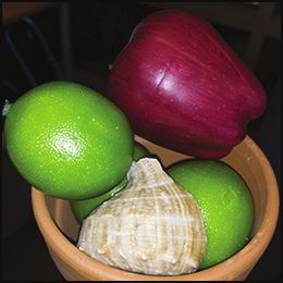
269:2 •      Zhengqin Li, Zexiang Xu, Ravi Ramamoorthi, Kalyan Sunkavalli, and Manmohan Chandraker

This represents a significant advance over recent works that either                layer that also accounts for interreflections.1 While it is challenging
consider SVBRDF estimation from near-planar samples [Aittala et al.                to directly predict the entire indirect component of an input image,
2016; Deschaintre et al. 2018; Li et al. 2017a, 2018], or estimate shape           we posit that predicting the bounces of global illumination using a
for Lambertian or homogeneous materials [Barron and Malik 2015;                    CNN is easier and maintains differentiability. Thus, our GI render-
Georgoulis et al. 2017; Liu et al. 2017]. The steep challenge of this              ing is implemented as a physically-motivated cascade, where each
goal requires a holistic approach that combines prudent image acqui-               stage predicts one subsequent bounce of global illumination. As a
sition, a large-scale training dataset, and novel physically-motivated             result, besides SVBRDF and shape, the individual bounces of global
networks that can efficiently handle this increased complexity.                    illumination are auxiliary outputs of our framework. A GI render-
   Several recent works have demonstrated that a collocated source-                ing layer also allows us to isolate the reconstruction error better,
sensor setup leads to advantages for material estimation, since                    thereby providing more useful feedback to the cascade structure.
higher frequencies for specular components are easily observed
                                                                                       Contributions. In summary, we make the following contributions:
and distractors such as shadows are eliminated [Aittala et al. 2016,
2015; Hui et al. 2017]. We use a mobile phone for imaging and mimic                •   The first approach to simultaneously recover unknown shape
this setup by using the flash as illumination. Note that our images                    and SVBRDF using a single mobile phone image.
are captured under uncontrolled environment illumination, and not                  •   A new large-scale dataset of images rendered with complex
a dark room. Our only assumption is that the flash illumination is                     shapes and spatially-varying BRDF.
dominant, which is true for most scenarios.                                        •   A novel cascaded network architecture that allows for global
   Previous inverse rendering methods have utilized 3D shape repos-                    reasoning and iterative refinement.
itories with homogeneous materials [Liu et al. 2017; Rematas et al.                •   A novel, physically-motivated global illumination rendering layer
2016; Shi et al. 2017] or large-scale SVBRDFs with near-planar ge-                     that provides more accurate reconstructions.
ometries [Deschaintre et al. 2018; Li et al. 2018]. While we utilize the
                                                                                   2    RELATED WORK
SVBRDF dataset of [Li et al. 2018], meaningfully applying them to 3D
models in a shape dataset is non-trivial. Moreover, category-specific              Inverse rendering — the problem of reconstructing shape, reflectance,
biases in repositories such as ShapeNet [Chang et al. 2015] might                  and lighting from a set of images — is an extensively studied prob-
mitigate the generalization ability of our learned model. To over-                 lem in computer vision and graphics. Traditional approaches to
come these limitations, we procedurally generate random shapes by                  this problem often rely on carefully designed acquisition systems
combining basic shape primitives on which the complex SVBRDFs                      to capture multiple images under highly calibrated conditions [De-
from our dataset are mapped. We generate a large-scale dataset of                  bevec et al. 2000]. Significant research has also been done on the
216, 000 images with global illumination that reflects the distribution            subproblems of the inverse rendering problem: e.g., photometric
of flash-illuminated images under an environment map.                              stereo methods that reconstruct shape assuming known reflectance
   Besides more descriptive datasets, disambiguating shape and                     and lighting [Woodham 1980], and BRDF acquisition methods that
spatially-varying material requires novel network architectures that               reconstruct material reflectance assuming known shape and light-
can reason about appearance at multiple scales, for example, to un-                ing [Marschner et al. 1999; Matusik et al. 2003]. While recent works
derstand both local shading and non-local shadowing and lighting                   have attempted to relax these assumptions and enable inverse ren-
variations, especially in the case of unknown, complex geometry. We                dering in the “wild”, to the best of our knowledge, this paper is
demonstrate that this can be achieved through a cascade design; each               the first to estimate both complex shape and spatially-varying non-
stage of the cascade predicts shape and SVBRDF parameters, but                     Lambertian reflectance from a single image captured under largely
these predictions and the error between images rendered with these                 uncontrolled settings. In this section, we focus on work that addresses
estimates and the input image are passed as inputs to subsequent                   shape and material estimation from sparse images.
stages. This allows the network to imbibe this global feedback on
the rendering error, while performing iterative refinement through                    Shape and material estimation. Shape from shading methods re-
the stages. In experiments, we demonstrate through quantitative                    construct shape from single images captured under calibrated illumi-
analysis and qualitative visualizations that the cascade structure is              nation, though they usually assume Lambertian reflectance [Johnson
crucial for accurate shape and SVBRDF estimation.                                  and Adelson 2011]. This has been extended to arbitrary shape and
   The forward rendering model is well-understood in computer                      reflectance under known natural illumination [Oxholm and Nishino
graphics, and can be used to aid the inverse problem by using a                    2016]. Shape and reflectance can also be estimated from multiple im-
fixed, in-network rendering layer to render the predicted shape and                ages by using differential motion cues [Chandraker 2014], light field
material parameters and impose a “reconstruction” loss during train-               inputs [Li et al. 2017b; Wang et al. 2017], or BRDF dictionaries [Gold-
ing [Deschaintre et al. 2018; Innamorati et al. 2017; Li et al. 2018;              man et al. 2010; Hui and Sankaranarayanan 2017]. Recent works
Liu et al. 2017; Shu et al. 2017; Tewari et al. 2018]. Tractable training          mitigate the challenge of shape recovery by using depth maps from
requires efficient rendering layers; thus, most previous works only                a Kinect sensor as input for BRDF estimation [Knecht et al. 2012; Wu
consider appearance under direct illumination. This is insufficient,               and Zhou 2015]. Other methods assume near-planar samples and
especially when dealing with arbitrary shapes. An important techni-                use physics-based optimization to acquire spatially-varying BRDFs
cal innovation of our network is a global illumination (GI) rendering              from sparse images captured under collocated illumination [Aittala
                                                                                   1 While itis possible to also consider shadows, global illumination is mainly manifested
                                                                                   as interreflections in our inputs due to the collocated setup.

ACM Trans. Graph., Vol. 37, No. 6, Article 269. Publication date: November 2018.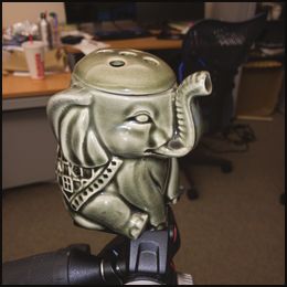
Learning to Reconstruct Shape and Spatially-Varying Reflectance from a Single Image • 269:3

et al. 2015; Hui et al. 2017; Riviere et al. 2016]. Yu et al. [1999] assume   2018; Li et al. 2018; Liu et al. 2017]. However, these methods make
known geometry to recover scene reflectance by modeling global                simplifying assumptions — usually Lambertian materials under dis-
illumination. Barron and Malik [2015] recover shape and spatially-            tant direct lighting or planar surface with collocated point lighting
varying diffuse reflectance from a single image under unknown                 — to make these layers tractable. We also use rendering to introduce
illumination by combining an inverse rendering formulation with               information from varied lighting conditions, but in contrast to the
hand-crafted priors on shape, reflectance and lighting. In contrast           above works, our rendering accounts for global illumination. Since
to these works, our deep learning approach recovers high-quality              analytical rendering of global illumination is challenging, we rely
shape and spatially-varying reflectance from a single RGB image by            on network modules to predict bounces of global illumination. The
combining a rendering layer with purely data-driven priors.                   idea of using a network to predict global illumination has also been
                                                                              adopted by [Nalbach et al. 2017], but no prior method has done this
   Deep learning for inverse rendering. Recently, deep learning-based
                                                                              for inverse problems. Further, we use a physically meaningful net-
approaches have demonstrated promising results for several in-
                                                                              work structure that divides global illumination into several bounces
verse rendering subproblems including estimating scene geome-
                                                                              instead of directly predicting indirect lighting, which may lead to
try [Bansal et al. 2016; Eigen and Fergus 2015], material classes [Bell
                                                                              better and more interpretable results. A deep network is also used
et al. 2015], illumination [Gardner et al. 2017; Georgoulis et al. 2017;
                                                                              by [Marco et al. 2017] to compensate for global illumination in time-
Hold-Geoffroy et al. 2017], and reflectance maps [Rematas et al.
                                                                              of-flight measurements, but they use a black box network for depth
2016]. In contrast, our work tackles the joint problem of estimating
                                                                              prediction while we model global illumination explicitly. There is
shape and spatially-varying reflectance from just a single image.
                                                                              machinery to compensate for bounces in optimization-based meth-
   In the context of reflectance capture, Aittala et al. [2016] propose
                                                                              ods [Godard et al. 2015], but they do not render in real-time and
a neural style transfer approach to acquire stochastic SVBRDFs from
                                                                              there is no obvious way to back-propagate gradients, making them
images of near-planar samples under flash illumination. Similarly,
                                                                              unsuitable for our framework. We train a global illumination CNN
Li et al. [2017a] acquire SVBRDFs from near-planar samples imaged
                                                                              to predict multiple bounces using data generated using a novel
under environment lighting, using a self-augmentation method
                                                                              simulation-based strategy that renders random shapes with a large-
to overcome the limitation of learning from a small dataset. Liu
                                                                              scale SVBRDF dataset. The use of random shapes is important, since
et al. [2017] propose a CNN-based method, that incorporates an
                                                                              we aim to recover arbitrary geometry, unlike previous methods that
in-network rendering layer, to reconstruct a homegenous BRDF
                                                                              might incorporate semantic category-level priors [Chang et al. 2015;
and shape (from one of four possible categories) from a single im-
                                                                              Georgoulis et al. 2017; Liu et al. 2017; Meka et al. 2018; Rematas et al.
age under unknown environment illumination. [Innamorati et al.
                                                                              2016]. Besides higher accuracy in SVBRDF estimation, a collateral
2017] use deep networks to decompose images into intrinsic compo-
                                                                              benefit of our novel rendering layer is that it can predict individual
nents like diffuse albedo, irradiance, specular and ambient occlusion,
                                                                              bounces of global illumination, in the same forward pass. These can
which are recombined to specify a render loss. We use a similar
                                                                              be subsequently used for scene analysis tasks [Nayar et al. 2006;
render loss, though our decomposition is physically-based. Meka
                                                                              O’Toole and Kutulakos 2010].
et al. [2018] recover homogeneous BRDF parameters of an arbi-
trary shape under environment lighting, and Li et al. [2018] and                 Cascade networks. For prediction tasks that demand sub-pixel
Deschaintre et al. [2018] leverage in-network rendering layers to             accuracy, prior works have considered cascade networks. For in-
reconstruct SVBRDFs from near-planar samples captured under                   stance, convolutional pose machines [Wei et al. 2016] are devised
flash illumination. Our work can be considered a generalization of            to obtain large receptive fields for localizing human body joints,
all these methods — we handle a broader range of SVBRDFs and                  while other architectures such as deep pose [Toshev and Szegedy
arbitrary shapes. This not only places greater demands on our net-            2014] and stacked hourglass networks [Newell et al. 2016] also use
work, but also necessitates the consideration of global illumination,         cascades for multiscale refinement. Improved optical flow estimates
leading to two key aspects of our architecture. First, we progres-            are obtained by FlowNet 2.0 [Ilg et al. 2017] using cascaded FlowNet
sively refine shape and SVBRDF estimates through a novel cascade              modules that accept stage-wise brightness error as input. Similar
design. Second, while previous in-network rendering layers [De-               to the above, we show that the cascade structure is effective for
schaintre et al. 2018; Li et al. 2018; Liu et al. 2017] only consider         SVBRDF estimation. Uniquely, we demonstrate that our cascade
direct illumination, our global rendering layer accounts for indirect         is sufficient to recover high-quality shape and SVBRDF, while our
illumination too. This not only matches our inputs better, but is also        global illumination prediction that enables rendering error as input
the more physically accurate choice for real scenes with complex              to the cascade stages also yields advantages for SVBRDF estimation.
shapes. Further, the rendering error provided as input to our cas-
cade stages improves estimation results, which is also possible only          3   METHOD
with a rendering layer that computes global illumination. Together,
                                                                              The input to our method is a single image of an object (with a mask)
these components leads to state-of-the-art results on a significantly
                                                                              captured under (dominant) flash and environment illumination. Re-
broader range of inputs.
                                                                              constructing spatially-varying BRDF (SVBRDF) and shape, in such
  Rendering layers in deep networks. Differentiable rendering layers          uncontrolled settings, is an extremely ill-posed problem. Inspired
have been used to aid in the task of learning inverse rendering for           by the recent success of deep learning methods in computer vision
problems like face reconstruction [Sengupta et al. 2018; Shu et al.           and computer graphics, we handle this problem by training a CNN
2017; Tewari et al. 2018] and material capture [Deschaintre et al.            specifically designed with intuition from physics-based methods. In

                                                                                  ACM Trans. Graph., Vol. 37, No. 6, Article 269. Publication date: November 2018.
269:4 • Zhengqin Li, Zexiang Xu, Ravi Ramamoorthi, Kalyan Sunkavalli, and Manmohan Chandraker
: Concatenate
Global illumination
: Branch
: No intersection
c256-k4-s2-d1
c128-k4-s2-d1
c256-k4-s2-d1
c512-k4-s2-d1
c512-k4-s2-d1
c256-k4-s2-d1
c256-k4-s2-d1
c128-k6-s2-d3
c128-k6-s2-d3
c32-k6-s2-d1
c64-k6-s2-d3
c64-k6-s2-d3
c32-k4-s2-d1
c32-k6-s2-d1
c64-k4-s2-d1
c64-k4-s2-d1
c32-k4-s2-d1
c3-k5-s1-d1
c256-k4-s2-
c128-k4-s2-
c3-k5-s1-d1
c128-k4-s2-
c256-k4-s2-
Albedo Albedo
Direct Rendering Layer
Normal Normal InverseNet GINet
Error Layer
Input
R-c128-k3-s2-d2
c512-k4-s2-d1 c128-k4-s2-d2
c256-k4-s2-d2 9 coefficients for
Rough Rough c1024-k4-s2-
each RGB color
c512-k3-s2-d2
Encoder f1024-drop0.25 c512-k3-s2-d2 f512-Drop0.25
R-c128-k3-s1-d2
R-c128-k3-s1-d2
R-c128-k3-s1-d2
R-c128-k3-s1-d2
R-c128-k3-s1-d2
R-c128-k3-s1-d2
Encoder
c128-k6-s2-d1
c64-k6-s2-d1
c64-k4-s2-d1
AvgPool-k4
c3-k5-s1-d1
f27 f512
c64-k4-s2-
Concatenat
9 coefficients for
Depth Depth f1024-Drop0.25
each RGB color
f512
InverseNet-Env 9 coefficients for
each RGB color
Env Env CascadeNet CascadeNet-Env
Fig. 2. Right: Overall structure of our framework. Different colors specify different functions of the network (blue for initial estimation, green for refinement
and purple for global illumination prediction). We use a cascade of encoder-decoder networks for global reasoning and iterative refinement. Different cascade
levels do not share parameters since the input statistics at each stage and the refinements needed are different. Each cascade stage receives error feedback
through the rendered output of the previous stage. Since we handle arbitrary shapes, our rendering layer models individual bounces of global illumination.
Left: Details of hyperparameters in our physically-motivated network design. Here R represents a residual block [He et al. 2016]. cX 1 −kX 2 −sX 3 −dX 4
represents a conv/deconv layer of output channel X 1 , kernel size X 2 , stride X 3 and dilation X 4 . Our encoder has receptive fields large enough to model global
light illumination, skip links are added since we aim to recover fine details and large kernels are used for global illumination prediction.
this section, we will describe each component of our network. The 3.2 Global Illumination Rendering Layer
overall framework is shown in Figure 2. Prior works on material capture or photometric stereo usually as-
sume that the influence of inter-reflections can be neglected, or
3.1 Basic Architecture consider near-planar samples where its effects are not strong. How-
Our basic network architecture consists of a single encoder and four ever, that may not be the case for our setup, since we consider
decoders for different shape and SVBRDF parameters: diffuse albedo complex shape with potentially glossy reflectance. Failing to model
(A), specular roughness (R), surface normal (N ), and depth (D).2 For global illumination for our problem can result in color bleeding and
simplicity, we start by considering the input to be an image, I p , of an flattened normal artifacts. We initially considered in-network global
object illuminated by a dominant point light source collocated with illumination rendering during training, but found it time-consuming
the camera (we consider additional environment illumination in and not feasible for a large dataset. Instead we propose using CNNs
Section 3.3). We manually create a mask, M, that we stack with the to approximate global illumination. CNNs can capture the highly
image to form a four channel input for the encoder. A light source non-linear operations that global illumination manifests. In addition,
collocated with the camera has the advantages of removing cast they have the advantage of being differentiable and fast to evaluate.
shadows, simplifying the lighting conditions and easing observation In particular, we use a series of CNNs, each of which predict indi-
of high frequency specularities, which are crucial for solving the vidual bounces of the rendered image. Let GINetn be the n-bounce
inverse rendering problem. In our experiments, such input data is CNN. This network is trained to takes the (n − 1)-bounce image
p
easily acquired using a mobile phone with the flash light enabled. under point light illumination, In−1 , and the shape and SVBRDF
Unlike [Li et al. 2017a], which has different encoders and decoders p
parameters, and render the n-bounce image, I˜n , as:
for various BRDF parameters, our four decoders share features ex-
p p
tracted from the same encoder. The intuition behind this choice is I˜n = GINetn (In−1 , M, A, N , R, D) (2)
that different shape and SVBRDF parameters are closely correlated,
thus, sharing features can greatly reduce the size of the network We use an analytical rendering layer to compute the direct illu-
p
and alleviate over-fitting. This architecture has been proven to be mination, i.e., first bounce image, I˜1 , given the predicted shape
successful in [Li et al. 2018] for material capture using near-planar and SVBRDF parameters. Then we use two CNNs, GINet2 (·) and
p p
samples. Let InverseNet(·) be the basic network architecture consist- GINet3 (·), to predict the second and third bounces, I˜2 and I˜3 re-
p
ing of the encoder-decoder block (shown in blue in Figure 2). Then spectively. The output, I˜д , of our full global illumination rendering
the initial predicted shape and SVBRDF estimates (differentiated layer (shown in purple in Figure 2) sums all the bounce images as:
from the true parameters by ˜ ) are given by:
p p
I˜2 = GINet2 (I˜1 , M, Ã, Ñ , R̃, D̃),
Ã, Ñ , R̃, D̃ = InverseNet(I p , M). (1) p p
I˜3 = GINet3 (I˜2 , M, Ã, Ñ , R̃, D̃),
2A specular albedo may be considered too, but we found it sufficient to consider just p p p p
roughness to mimic most real-world appearances. I˜д = I˜1 + I˜2 + I˜3 . (3)
ACM Trans. Graph., Vol. 37, No. 6, Article 269. Publication date: November 2018.
Learning to Reconstruct Shape and Spatially-Varying Reflectance from a Single Image • 269:5

                                                                             both point and environmental lighting and M ⊙ I pe be its masked
                                                                             version. With some abuse of notation, now our shape and SVBRDF
                                                                             parameters are computed using
                                                                                            Ã, Ñ , R̃, D̃, Ẽ = InverseNet(I pe , M ⊙ I pe , M).              (4)
                                                                             Since now the input image is captured under environment illumi-
                                                                             nation and the flash light source, we modify our rendering layer
                                                                             to account for this. We follow the method of [Ramamoorthi and
                                                                             Hanrahan 2001] to render an image of the object, I˜e , using the es-
                                                                             timated spherical harmonics illumination. This only considers the
                                                                             Lambertian shading and ignores high-frequency specular effects.
                  1st bounce     2nd bounce      3r d bounce     others      In practice, this is sufficient because most high-frequency effects
 Energy ratio       95.83%          3.08%            0.89%       0.20 %      are observed under flash illumination, and our experiments show
                                                                             that this simple approximation suffices for achieving accurate BRDF
Fig. 3. Global illumination prediction results. From left to the right are   reconstruction. Now the output of the global illumination rendering
input images, the predicted second bounce images, the ground truth second
                                                                             layer (in place of Equation 3) is given by:
bounce images, the predicted third bounce images and the ground truth
                                                                                                           pe    p     p     p
third bounce images. Even for complex shapes with glossy material, the                                   I˜д = I˜1 + I˜2 + I˜3 + I˜e .                          (5)
predictions of our network are close to the ground truth. On the bottom,
we show the ratio between the average energy of separate bounces and the     3.4      Cascade Structure
images illuminated by a point light source across the test dataset.          While a single encoder-decoder leads to good results for SVBRDF
                                                                             estimation with near-planar samples [Li et al. 2018], it does not
                                                                             suffice when considering arbitrary shapes. This can be attributed to
   As illustrated in Figure 3, most of the image intensity is contained
                                                                             the increased complexity of the problem and a need for more global
within three bounces, and so we only predict these, ignoring sub-
                                                                             reasoning. We propose a cascade structure that achieves these aims
sequent bounces. Also in Figure 3, we show second and the third
                                                                             by using iterative refinement and feedback to allow the network
bounce images predicted by our network. We observe that even for
                                                                             to reason about differences between the image rendered with the
objects with very concave shape and highly glossy material, we can
                                                                             predicted parameters and the input image.
still generate rendering outputs that closely match the ground truth.
                                                                                 Let CascadeNetn be stage n of the cascade network. Each stage
   Note that a CNN-based approach like ours only approximates
                                                                             has the same single architecture as InverseNet. Let the shape, re-
true global illumination. It operates in image space and does not
                                                                             flectance and lighting parameters of cascade stage n be Ãn , Ñn , R̃n ,
explicitly model interreflections from surface points that are not
                                                                             D̃ n and Ẽn , and the result of rendering these parameters (using the
visible to the camera. However, our training data does include inter-                                                       pe
                                                                             global illumination rendering network) be I˜д,n . Each cascade stage
reflections from invisible surfaces and our collocated setup causes
                                                                             refines the predictions of the previous stage as:
interreflections from visible regions to dominate. In practice, we
                                                                                                                           pe
have found the network to be sufficiently accurate for inverse ren-                                 Err n−1 = M ⊙ I pe − I˜д,n−1                                (6)
dering. Compared with the traditional radiosity method [Cohen and                                                                     pe            pe
                                                                                     Ãn , Ñn , R̃n , D̃ n , Ẽn = CascadeNetn (I         ,M ⊙ I        , M,
Wallace 1993], our network-based global illumination prediction has
the advantage of being fast, differentiable and able to approximate                                                Ãn−1 , Ñn−1 , R̃n−1 , D̃ n−1 , Err n−1 )   (7)
reflections from invisible surfaces. However, it is an approximation,           The inputs to each cascade stage are the input image, the shape,
since we do not have precise geometry, form factors or material              SVBRDF, and lighting predictions from the previous stage, and the
(albedo) properties, as in conventional radiosity algorithms.                rendering error associated with these previous predictions (with
                                                                             respect to the input image). This allows each cascade stage to refine
3.3   Environment Map Prediction                                             the predictions by reasoning about the rendering error from the
Although we use a dominant flash light, our images are also illu-            previous stage. Note that this is possible only because of our network
minated by unknown environment illumination. This environment                design that models global illumination and environment lighting.
illumination can significantly affect the appearance of globally illu-
minated complex shapes. This requires us to estimate the environ-            3.5      Training Details
ment illumination and account for it in our rendering networks. To              Training Data: To the best of our knowledge, there is no exist-
do so, we approximate environment lighting with low-frequency                ing dataset of objects with arbitrary shape rendered with complex
spherical harmonics (SH), and add another branch to our encoder-             SVBDRF. Complex SVBRDF datasets used in previous work [De-
decoder structure to predict the first nine SH coefficents for each          schaintre et al. 2018; Li et al. 2018] assume near-planar surfaces, and
color channel. We observe that the background image provides                 rich shape datasets like ShapeNet [Chang et al. 2015] have simple
important context information for the network to determine en-               homogeneous BRDFs. Thus, we generate our own synthetic dataset
vironment lighting. So, unlike the point light source case, we add           by procedurally adding shapes to build a complex scene. Similar
the image with background as the third image to the input. Let               to [Xu et al. 2018], we first generate primitive shapes (cube, ellip-
E be environment lighting, I pe be the image of the object under             soid, cylinder, box and L-shape) and then add a randomly generated

                                                                                   ACM Trans. Graph., Vol. 37, No. 6, Article 269. Publication date: November 2018.
269:6 •       Zhengqin Li, Zexiang Xu, Ravi Ramamoorthi, Kalyan Sunkavalli, and Manmohan Chandraker

height map to make them more complex and diverse. We build                           Loss function: We have the same loss function for both InverseNet
scenes by randomly sampling 1 to 5 shapes and combining them.                      and each CascadeNet stage. For diffuse albedo, normal, roughness
We create 3600 scenes, using 3000 for training and 600 for testing.                and environment illumination SH coefficients, we use the L2 loss for
   We use SVBDRFs from the Adobe Stock material dataset3 , which                   supervision. Since the range of depths is larger than that of other
contains 694 complex SVBRDFs spanning a large range of material                    BRDF parameters, we use an inverse transformation to project the
types. Each SVBRDF is comprised of 4K texture maps for diffuse                     depth map into a fixed range. Let d˜i be the initial output of depth
albedo, specular roughness, and surface normals. For data augmen-                  prediction network of pixel i; the real depth di is given by
tation, we randomly crop, rotate and scale the texture maps to create                                                     1
different size patches and then resize all the patches to the same                                          di =                       .               (8)
                                                                                                                   σ · (d˜i + 1) + ϵ
size of 256 × 256. We create 270 patches for each material and use
these patches as the materials to render dataset. We use the physi-                We set σ = 0.4 and ϵ = 0.25, and use L2 loss to supervise di . Finally,
cally motivated microfacet BRDF model in [Karis and Games 2013].                   we add a reconstruction loss based on the L2 distance between
Please refer to the supplementary material for details.                            the image rendered with predicted and ground truth parameters.
   We remove the 6 transparent materials and use the remaining 688                 Let La , Ln , Lr , Ld , Lenv and Lr ec be the L2 losses for diffuse
materials. We classify the materials into 8 categories according to                albedo, normal, roughness, depth, environment map and image
their reflectance properties and proportionally sample 588 materials               reconstruction, respectively. The loss function of our network is:
for training and 100 for testing. For environment maps, we use the                     L = λa La + λn Ln + λr Lr + λd Ld + λenv Lenv + λr ec Lr ec , (9)
Laval Indoor HDR dataset [Gardner et al. 2017] containing 2144
environmental maps of indoor scenes, of which we use 1500 to                       where λa = λn = λr ec = 1, λr = λd = 0.5 and λenv = 0.1 are
render the training dataset and 644 for the test dataset.                          parameters chosen empirically.
   We use Optix for GPU-accelerated rendering, based on path trac-                    Training Strategies: Training multiple cascade structures is dif-
ing with multiple importance sampling. We render with 400 samples                  ficult since the enhanced network depth may lead to vanishing
per-pixel for point light source illumination and 625 samples per-                 gradients and covariate shift, preventing convergence to a good
pixel when the environment map is also included. The average                       local minimum. Further, batch sizes will need to be small when
rendering time is less than 2 seconds. For each scene, we sample                   training all stages together, which can cause instability. Thus, in-
12 viewing directions, 5 groups of different SVBDRFs and one en-                   stead of training the whole network end-to-end, we sequentially
vironment map. When rendered with both point and environment                       train each stage of the cascade. This allow us to use a relatively large
lighting, we scale the environment map by 0.5, to keep the average                 batch size of 16. We use Adam optimizer, with a learning rate of
ratio between image intensities rendered with only environment                     10−4 for the encoder and 4 × 10⁻⁴ for the decoders. We decrease the
map and with point light to be 0.09285. This matches the statistics of             learning rate by half after every two epochs. The three stages are
images captured using mobile phones in real indoor environments.                   trained for 15, 8 and 6 epochs, respectively. We use two CascadeNet
   Network Design: Our design makes several choices to reflect                     stages and train InverseNet and CascadeNet1 with 2500 shapes
the physical structure of the problem. We use the U-net architec-                  and add 500 shapes to train CascadeNet2 .
ture [Ronneberger et al. 2015] for InverseNet. To model the global                    GINet is trained prior to the BRDF prediction network, then
fall-off of the point light source, it is necessary to have large recep-           held fixed and only used for the rendering layer when training the
tive fields. Thus, each encoder has 6 convolutional layers with stride             network for shape and SVBRDF estimation. We use Optix to render
2, so that each pixel of the output can be influenced by the whole                 images with separate bounces and use them for direct supervision.
image. For the SVBDRF parameters, we use transposed convolu-                       We train for 15 epochs, with an initial learning rate of 2 × 10⁻⁴ and
tions for decoding and add skip links to recover greater details. For              reduce it by half every two epochs.
environment map estimation, we pass the highest level of feature
                                                                                   4     EXPERIMENTS
extracted from the encoder through two fully connected layers to
regress the 9 spherical harmonics coefficients. Each CascadeNet                    We first demonstrate the effectiveness of each design choice in our
stage uses 6 residual blocks — 3 blocks for the encoder and 3 sep-                 network architecture through detailed comparisons on both syn-
arate blocks for each decoder. We use dilated convolutions with a                  thetic and real datasets. Next, we compare with previous methods
factor of 2 in the residual block to increase the receptive field. We              for shape and material estimation to highlight the highly accurate
feed environment lighting predictions into the next cascade stage by               shape and SVBRDF recovered by our framework. Please refer to sup-
passing the nine SH coefficients through a fully connected layer and               plementary video for more visualizations of the results (including
concatenate them with the feature extracted from the encoder. We                   under novel lighting and viewpoint).
also use the U-net structure with skip-links for GINet. To predict                    Ablation study on synthetic data. We first justify the necessity
global illumination, the network must capture long range depen-                    of rendering a novel large-scale dataset with global illumination
dencies. Thus, we use a convolutional layer with large kernel of size              for shape and SVBRDF estimation. We train InverseNet on images
6, combined with dilation by a factor of 2. The network architecture               rendered with direct illumination and test on images with global
of each component is shown on the right side of Figure 2.                          illumination. Column Impd −C0 (trained on images with direct point
                                                                                   illumination with no cascade) in Table 1 reports the obtained errors,
3 https://stock.adobe.com/3d-assets
                                                                                   which are clearly larger than those in column Impg −C0 for the same

ACM Trans. Graph., Vol. 37, No. 6, Article 269. Publication date: November 2018.
Learning to Reconstruct Shape and Spatially-Varying Reflectance from a Single Image • 269:7

Table 1. Quantitative comparison on images rendered only with point light.           Input image              eBgIm-C 2 E NoG   eBgIm-C 2 E       Ground truth

Impd refers to input images rendered with direct lighting only, while Impg
means the input images are rendered with global illumination.

                                            Impd −C0   Impg −C0
                         Albedo(10−2 )

                                                                                                     Albedo
                                             5.911      5.703
                                                                                     GI prediction
                         Normal(10−2 )       4.814      4.475
                         Roughness(10−1 )    1.974      1.966
                         Depth(10−1 )        1.842      1.772

                Albedo            Normal        Roughness         Depth

                                                                                Fig. 5. For an input image with strong indirect lighting (top left), a network
 dIm-C0

                                                                                trained without global illumination for the rendering layer (second column)
                                                                                retains more color bleeding artifacts in the estimated diffuse albedo, than
                                                                                one trained with global illumination (third column). The bottom left figure
                                                                                shows the net global illumination estimated by the final network.
 iIm-C 0

                                                                                another cascade stage with error feedback, which yields even more
                                                                                accurate BRDF estimation (C2 Er) that we deem the final output.
                                                                                Figure 6 shows the visual quality of BRDF estimation from different
 Ground truth

                                                                                stages of the cascade network. We observe that for both synthetic
                                                                                and real data, the cascade reduces noise and artifacts. The final
                                                                                rendered result using the BRDF parameters predicted by the second
                                                                                level of the cascade is very similar to the input image, as shown in
                                                                                Figure 6 using both the environment map estimated by the network
Fig. 4. Comparison of SVBRDF and depth outputs of two networks, trained         and a novel environment map.
on directly illuminated (top) and globally illuminated images (middle), when       Next, we analyze the effect of the global illumination rendering
evaluated on an input with global illumination. Not considering indirect        network. We train two new variants of our global illumination ren-
lighting during training leads to flatter normals and brighter albedo.          dering layer for the second cascade stage. For Impe          g −bg−C2 ErNoG ,
                                                                                the rendering layer does not consider global illumination so that the
                                                                                                                                                p
                                                                                error feedback is computed by subtracting the sum of I˜1 and I˜e from
network trained on images with point lighting and global illumina-                                                 p
                                                                                the input M ⊙I pe , i.e., I˜pe = I˜1 +I˜e . Similarly, for Impe
                                                                                                                                             g −bg−C2 ErNoE ,
tion. Thus, global illumination has a significant impact on depth and           we remove the environmental map component of the global illumi-
SVBRDF estimation. The qualitative comparison in Figure 4 shows                 nation rendering layer. The error feedback for the cascade network
that the network trained with direct lighting only predicts brighter                                                  p       p   p
                                                                                is now computed using I˜pe = I˜1 + I˜2 + I˜3 . Table 2 shows that our
diffuse albedo and flattened normals, when evaluated on images
                                                                                full version of rendering layer performs the best. The differences
with indirect lighting. This also matches intuition on the behavior
                                                                                are measurable but subtle, since the remaining impact of environ-
of inter-reflections [Chandraker et al. 2005; Nayar et al. 1991].
                                                                                ment lighting and global illumination for the second stage is small.
   Next we demonstrate that context information is important for
                                                                                To better understand the behavior, we show a qualitative example
the network to reconstruct shape and BRDF under environment
                                                                                with global illumination in Figure 5. We observe that the global
lighting. We train two variants of our basic network, one with
                                                                                illumination rendering layer alleviates color bleeding artifacts.
masked image input, Impe g −C0 , and the other with both masked and
original image as input, Impe
                            g −bg−C0 . Quantitative comparisons in                 Generalization to real data. We demonstrate our method on sev-
the first two columns of Table 2 show that predictions for all BRDF             eral real objects in Figures 7 and 8. All images are captured in indoor
parameters improve when background is included.                                 scenes using an iPhone 10 with the flash enabled. We use the Adobe
   To test the effectiveness of cascade structure, we first add one             Lightroom app to capture linear images and manually create the seg-
layer of cascade to our basic network. We try two variants of cascade           mentation mask. For all the examples, our rendered results closely
network. For the black-box cascade (C1 ), we stack the input image              match the input. Figures 7 and 8 also show our predicted BRDF
and the predicted BRDF parameters and send them to the next stage               parameters can be used to render realistic images under new en-
of the cascade. For the cascade network with error feedback (C1 Er),            vironment lighting and camera pose. This demonstrates that our
we also send an error map as input by comparing the output of our               estimates of the surface normal and spatially varying roughness are
global illumination rendering layer with the input. The quantitative            of high enough quality to render realistic specular effects of real
numbers (third and fourth column of Table 2) suggest that having                objects under novel illumination and viewing directions. Please see
the error feedback improves BRDF reconstruction. We then add                    the supplementary material and videos for further examples.

                                                                                   ACM Trans. Graph., Vol. 37, No. 6, Article 269. Publication date: November 2018.
269:8 •                   Zhengqin Li, Zexiang Xu, Ravi Ramamoorthi, Kalyan Sunkavalli, and Manmohan Chandraker

Table 2. Quantitative comparisons L2 errors illustrating the influence of various network choices. Impe
                                                                                                      g means the input images are illuminated by both point
light source and environmental lighting (superscript pe) and rendered with global illumination (subscript g).−bg means the images without masking the
background are added as an input. Cn shows the level of cascade refinement, where C0 means we use our basic InverseNet without any refinement. Er behind
Cn means we also send the error maps by comparing the images rendered with the estimated BRDFs and the inputs to the cascade refinement networks. The
subscript NoE and NoG in the last two columns means that when computing the error maps, we do not consider the influence of environmental lighting and
global illumination respectively. Here, Impe
                                          g −bg−C2 Er is the error obtained with our final two-cascade architecture with global illumination and error feedback.

                                        Impe
                                          g −C0    Impe
                                                     g −bg−C0   Impe
                                                                  g −bg−C1         Impe
                                                                                     g −bg−C1 Er   Impe
                                                                                                     g −bg−C2 Er   Impe
                                                                                                                     g −bg−C2 ErNoE          Impe
                                                                                                                                               g −bg−C2 ErNoG
   Albedo(10−2 )                         6.089        5.670        5.150                5.132           4.868            4.900                     4.880
   Normal(10−2 )                         4.727        4.580        3.929                3.907           3.822            3.830                    3.822
   Roughness(10−1 )                      2.207        2.064        2.004                2.011           1.943            1.948                     1.947
   Depth(10−2 )                          1.945        1.871        1.631                1.624           1.505            1.512                     1.511
   Bounce 1(10−3 )                       3.526        3.291        2.190                2.046           1.637            1.643                     1.643
   Bounce 2(10−4 )                        2.88         2.76         2.47                 2.47           2.45              2.45                      2.46
   Bounce 3(10−5 )                        6.6           6.4          5.9                5.9 .            5.8              5.8                       5.8

                              Initial             Cascade 1     Cascade 2          Ground truth         Initial          Cascade 1           Cascade 2
         Albedo
         Normal
         Roughness
         Depth

                                                                            0      0.5
         Rendered Image
        Rendered Image

                                                                                                                                     Input

Fig. 6. Effect of our cascaded design, illustrated for synthetic (left) and real data (right). It is observed that predictions from the initial network are somewhat
inaccurate, but progressively improved by the cascade stages. Images rendered after two cascade stages have less artifacts and display specular highlights
closer to the ground truth, both when relit with the estimated environment map and rendered under a new environment map. We visualize the absolute error
for the BRDF parameters in the third column except the depth error. The depth error is normalized so that the range of ground-truth depth is 1.

ACM Trans. Graph., Vol. 37, No. 6, Article 269. Publication date: November 2018.
Learning to Reconstruct Shape and Spatially-Varying Reflectance from a Single Image • 269:9

           Input          Rendered result      Diffuse albedo          Normal               Depth                  Roughness            Rendered Image

Fig. 7. Results on real objects. For each example, we show the input image, the rendered output using the estimated shape and BRDF parameters, as well as
visualization under a novel illumination condition. In each case, we observe high quality recovery of shape and spatially-varying BRDF.

           Input          Diffuse albedo          Normal               Depth               Roughness               Novel view 1            Novel view 2

Fig. 8. Results rendered from novel views. We show the input image, the estimated shape and BRDF parameters and the rendered output under an environment
map from two novel views. We observe high fidelity rendered images, as well as high quality recovery of shape and spatially-varying BRDF.

                                                                                   ACM Trans. Graph., Vol. 37, No. 6, Article 269. Publication date: November 2018.
269:10     • Zhengqin Li, Zexiang Xu, Ravi Ramamoorthi, Kalyan Sunkavalli, and Manmohan Chandraker

           Input                    Barron and Malik 2015   Ours                  Ground truth               Input               Barron and Malik 2015   Ours

                           Normal

                                                                                                                        Normal
                                                                                                                        Albedo
                           Albedo

Fig. 9. Comparison with SIRFS [Barron and Malik 2015]. Our method accurately estimates the shape and diffuse color, even in regions with specularity. In
contrast, because of the complex shape and materials of these objects, SIRFS, which assumes Lambertian reflectance, produces very inaccurate estimates.

   Comparisons with previous methods. Since we are not aware of                                 Limitations. A few challenges remain unaddressed. Our network
prior works that can use a single image for spatially varying BRDF                           does not explicitly handle improperly exposed images. For example,
and shape estimation, our comparisons are to more restricted meth-                           saturations from the flash may cause the specular highlight to be
ods for shape and material estimation, or to intrinsic image decom-                          baked into the diffuse color (such as the orange in the third row of
position methods. We first compare with SIRFS [Barron and Malik                              Figure 7). This problem might be solved by adding more training
2015] which jointly reconstructs shape and diffuse color. Figure 9                           data and using more aggressive data augmentation. As discussed pre-
compares the diffuse albedo and normal estimated using SIRFS with                            viously, long-range interactions might not be sufficiently modeled in
those obtained by our framework, on both real and synthetic data. In                         our image-space CNN, which may limit its ability to correctly han-
both cases, our estimates are significantly better. Notice that SIRFS                        dle interreflections. We find spatially varying roughness prediction
tends to over-smooth both the diffuse color and the normal due to                            to be a challenging problem. The presence of specular highlights is
a handcrafted regularization. In contrast, our method successfully                           important for it and the network may rely on connectivity priors
recovers high-frequency details for both diffuse albedo and surface                          to predict roughness. However, this prior may fail, which results in
normals, even in specular and shadowed regions.                                              the same material having different roughness values (such as the
                                                                                             owl in the second row of Figure 8). Such a prior might be explicitly
         Input            Shi et al. 2017            Ours          Ground truth
                                                                                             enhanced to improve performance by using a densely connected
                                                                                             CRF [Ristovski et al. 2013] or bilateral filter [Barron and Poole 2016].
                                                                                             Another possibility would be to take shape-material correlations
                                                                                             into account. From Figure 6, we can see that the error of depth
                                                                                             prediction is significantly larger than the normal prediction, which
                                                                                             suggests that we may use normal predictions to refine depth pre-
                                                                                             dictions [Nehab et al. 2005]. Despite these limitations, we note that
                                                                                             our network achieves significantly better results than prior works
                                                                                             on this challenging, ill-posed problem.

                                                                                                 5   CONCLUSION
                                                                                             We demonstrate the first approach for simultaneous estimation of
Fig. 10. Comparison with [Shi et al. 2017]. While Shi et al. train to handle
                                                                                             arbitrary shape and spatially-varying BRDF, using a single mobile
non-Lambertian reflectance, the accuracy and visual quality of our diffuse                   phone image. We make several physically-motivated and effective
albedo is significantly higher on both synthetic (top) and real data (bottom).               choices across image acquisition, dataset creation and network ar-
                                                                                             chitecture. We use a mobile phone flash to acquire images, which
                                                                                             allows observing high frequency details. Our large-scale dataset
   We also compare with the recent intrinsic image decomposition                             of procedurally created shapes, rendered with spatially-varying
method of [Shi et al. 2017], which is trained to separate diffuse                            BRDF under various lighting conditions, prevents entanglement of
and specular components from a single image of a ShapeNet object                             category-level shape information with material properties. Our cas-
[Chang et al. 2015], rendered under the assumption of a parametric                           caded network allows global reasoning through error feedback and
homogeneous BRDF. We compare to their diffuse albedo prediction                              multiscale iterative refinement, to obtain highly accurate outputs for
in Figure 10. Our method can better preserve occlusion boundaries                            both shape and material. We propose a novel rendering layer to in-
and recover accurate diffuse color even in specular regions. Our                             corporate information from various lighting conditions, which must
method also yields qualitatively superior results on real data.                              account for global illumination to handle arbitrary shape. Inspired

ACM Trans. Graph., Vol. 37, No. 6, Article 269. Publication date: November 2018.
Learning to Reconstruct Shape and Spatially-Varying Reflectance from a Single Image • 269:11
by the physical process of rendering bounces of global illumination, Martin Knecht, Georg Tanzmeister, Christoph Traxler, and Michael Wimmer. 2012.
we devise a cascaded CNN module that retains speed and simplicity. Interactive BRDF Estimation for Mixed-Reality Applications. WSCG 20, 1 (2012).
Xiao Li, Yue Dong, Pieter Peers, and Xin Tong. 2017a. Modeling surface appearance
Extensive experiments validate our network design through high- from a single photograph using self-augmented convolutional neural networks.
quality estimation of shape and SVBRDF that outperforms previous ACM Trans. Graphics 36, 4 (2017).
Zhengqin Li, Kalyan Sunkavalli, and Manmohan Chandraker. 2018. Materials for
methods. In future work, we will demonstrate applications of our Masses: SVBRDF Acquisition with a Single Mobile Phone Image. In ECCV.
framework to material editing and augmented reality, as well as Z. Li, Z. Xu, R. Ramamoorthi, and M. Chandraker. 2017b. Robust Energy Minimization
consider extensions to large-scale scenes such as room interiors. for BRDF-Invariant Shape from Light Fields. In CVPR.
Guilin Liu, Duygu Ceylan, Ersin Yumer, Jimei Yang, and Jyh-Ming Lien. 2017. Material
Editing using a Physically Based Rendering Network. ICCV.
ACKNOWLEDGMENTS Julio Marco, Quercus Hernandez, Adolfo Munoz, Yue Dong, Adrian Jarabo, Min H Kim,
Xin Tong, and Diego Gutierrez. 2017. DeepToF: off-the-shelf real-time correction of
We thank the reviewers for many helpful suggestions. This work multipath interference in time-of-flight imaging. ACM Trans. Graphics 36, 6 (2017).
was supported in part by NSF CAREER 1751365, NSF Grant 1703957, Stephen R Marschner, Stephen H Westin, Eric PF Lafortune, Kenneth E Torrance, and
ONR grant N000141712687, Adobe, the Ronald L. Graham Chair, Donald P Greenberg. 1999. Image-based BRDF measurement including human skin.
In Rendering Techniques.
and the UC San Diego Center for Visual Computing. Wojciech Matusik, Hanspeter Pfister, Matt Brand, and Leonard McMillan. 2003. A
Data-Driven Reflectance Model. ACM Trans. Graphics 22, 3 (2003).
REFERENCES Abhimitra Meka, Maxim Maximov, Michael Zollhoefer, Avishek Chatterjee, Hans-
Peter Seidel, Christian Richardt, and Christian Theobalt. 2018. LIME: Live Intrinsic
Miika Aittala, Timo Aila, and Jaakko Lehtinen. 2016. Reflectance modeling by neural Material Estimation. In CVPR.
texture synthesis. ACM Trans. Graphics 35, 4 (2016). Oliver Nalbach, Elena Arabadzhiyska, Dushyant Mehta, H-P Seidel, and Tobias Ritschel.
Miika Aittala, Tim Weyrich, Jaakko Lehtinen, et al. 2015. Two-shot SVBRDF capture 2017. Deep shading: convolutional neural networks for screen space shading.
for stationary materials. ACM Trans. Graphics 34, 4 (2015). Comput. Graph. Forum 36, 4 (2017).
Aayush Bansal, Bryan Russell, and Abhinav Gupta. 2016. Marr Revisited: 2D-3D Model Shree K. Nayar, Katsushi Ikeuchi, and Takeo Kanade. 1991. Shape from interreflections.
Alignment via Surface Normal Prediction. In CVPR. IJCV 6, 3 (1991).
Jonathan T Barron and Jitendra Malik. 2015. Shape, illumination, and reflectance from Shree K. Nayar, Gurunandan Krishnan, Michael D. Grossberg, and Ramesh Raskar. 2006.
shading. PAMI 37, 8 (2015). Fast Separation of Direct and Global Components of a Scene Using High Frequency
Jonathan T Barron and Ben Poole. 2016. The fast bilateral solver. In European Conference Illumination. ACM Trans. Graphics 25, 3 (2006).
on Computer Vision. Springer, 617–632. Diego Nehab, Szymon Rusinkiewicz, James Davis, and Ravi Ramamoorthi. 2005. Effi-
Sean Bell, Paul Upchurch, Noah Snavely, and Kavita Bala. 2015. Material Recognition ciently combining positions and normals for precise 3D geometry. In ACM transac-
in the Wild with the Materials in Context Database. In CVPR. tions on graphics (TOG), Vol. 24. ACM, 536–543.
Volker Blanz and Thomas Vetter. 1999. A morphable model for the synthesis of 3D Alejandro Newell, Kaiyu Yang, and Jia Deng. 2016. Stacked Hourglass Networks for
faces. In Proc. SIGGRAPH. Human Pose Estimation. In ECCV.
Manmohan Chandraker. 2014. On shape and material recovery from motion. In ECCV. Matthew O’Toole and Kiriakos N. Kutulakos. 2010. Optical Computing for Fast Light
Manmohan Chandraker, Fredrik Kahl, and David Kriegman. 2005. Reflections on the Transport Analysis. ACM Trans. Graphics 29, 6, Article 164 (2010).
generalized bas-relief ambiguity. In CVPR. Geoffrey Oxholm and Ko Nishino. 2016. Shape and reflectance estimation in the wild.
Angel X Chang, Thomas Funkhouser, Leonidas Guibas, Pat Hanrahan, Qixing Huang, PAMI 38, 2 (2016), 376–389.
Zimo Li, Silvio Savarese, Manolis Savva, Shuran Song, Hao Su, et al. 2015. Shapenet: Ravi Ramamoorthi and Pat Hanrahan. 2001. An efficient representation for irradiance
An information-rich 3d model repository. arXiv preprint arXiv:1512.03012 (2015). environment maps. In SIGGRAPH.
Michael F Cohen and John R Wallace. 1993. Radiosity and realistic image synthesis. Konstantinos Rematas, Tobias Ritschel, Mario Fritz, Efstratios Gavves, and Tinne Tuyte-
Elsevier. laars. 2016. Deep reflectance maps. In CVPR.
Paul Debevec, Tim Hawkins, Chris Tchou, Haarm-Pieter Duiker, Westley Sarokin, and Kosta Ristovski, Vladan Radosavljevic, Slobodan Vucetic, and Zoran Obradovic. 2013.
Mark Sagar. 2000. Acquiring the reflectance field of a human face. In SIGGRAPH. Continuous Conditional Random Fields for Efficient Regression in Large Fully
Valentin Deschaintre, Miika Aittala, Fredo Durand, George Drettakis, and Adrien Connected Graphs.. In AAAI.
Bousseau. 2018. Single-image SVBRDF Capture with a Rendering-aware Deep J. Riviere, P. Peers, and A. Ghosh. 2016. Mobile Surface Reflectometry. Comput. Graph.
Network. ACM Trans. Graph. 37, 4 (2018). Forum 35, 1 (2016).
David Eigen and Rob Fergus. 2015. Predicting depth, surface normals and semantic O. Ronneberger, P.Fischer, and T. Brox. 2015. U-Net: Convolutional Networks for
labels with a common multi-scale convolutional architecture. In ICCV. Biomedical Image Segmentation. In MICCAI.
Marc-André Gardner, Kalyan Sunkavalli, Ersin Yumer, Xiaohui Shen, Emiliano Gam- Soumyadip Sengupta, Angjoo Kanazawa, Carlos D. Castillo, and David W. Jacobs. 2018.
baretto, Christian Gagné, and Jean-François Lalonde. 2017. Learning to predict SfSNet: Learning Shape, Refectance and Illuminance of Faces in the Wild. In CVPR.
indoor illumination from a single image. ACM Trans. Graphics 9, 4 (2017). Jian Shi, Yue Dong, Hao Su, and Stella X Yu. 2017. Learning Non-Lambertian Object
Stamatios Georgoulis, Konstantinos Rematas, Tobias Ritschel, Mario Fritz, Tinne Tuyte- Intrinsics Across ShapeNet Categories. In CVPR.
laars, and Luc Van Gool. 2017. What is around the camera?. In ICCV. Z. Shu, E. Yumer, S. Hadap, K. Sunkavalli, E. Shechtman, and D. Samaras. 2017. Neural
Clement Godard, Peter Hedman, Wenbin Li, and Gabriel J Brostow. 2015. Multi-view Face Editing with Intrinsic Image Disentangling. In CVPR.
reconstruction of highly specular surfaces in uncontrolled environments. In 3DV. A. Tewari, M. Zollhofer, H. Kim, P. Garrido, F. Bernard, P. Perez, and C. Theobalt.
Dan B Goldman, Brian Curless, Aaron Hertzmann, and Steven M Seitz. 2010. Shape 2018. MoFA: Model-Based Deep Convolutional Face Autoencoder for Unsupervised
and spatially-varying brdfs from photometric stereo. PAMI 32, 6 (2010). Monocular Reconstruction. In ICCV.
Kaiming He, Xiangyu Zhang, Shaoqing Ren, and Jian Sun. 2016. Deep residual learning A. Toshev and C. Szegedy. 2014. DeepPose: Human Pose Estimation via Deep Neural
for image recognition. In CVPR. Networks. In CVPR.
Yannick Hold-Geoffroy, Kalyan Sunkavalli, Sunil Hadap, Emiliano Gambaretto, and Ting-Chun Wang, Manmohan Chandraker, Alexei Efros, and Ravi Ramamoorthi. 2017.
Jean-François Lalonde. 2017. Deep Outdoor Illumination Estimation. In CVPR. SVBRDF-Invariant Shape and Reflectance Estimation from Light-Field Cameras.
Z. Hui and A. C. Sankaranarayanan. 2017. Shape and Spatially-Varying Reflectance PAMI (2017).
Estimation from Virtual Exemplars. PAMI 39, 10 (2017). S. E. Wei, V. Ramakrishna, T. Kanade, and Y. Sheikh. 2016. Convolutional Pose Machines.
Zhuo Hui, Kalyan Sunkavalli, Joon-Young Lee, Sunil Hadap, Jian Wang, and Aswin C. In CVPR.
Sankaranarayanan. 2017. Reflectance capture using univariate sampling of BRDFs. Robert J. Woodham. 1980. Photometric Method For Determining Surface Orientation
In ICCV. From Multiple Images. Optical Engineering 19 (1980).
Eddy Ilg, Nikolaus Mayer, Tonmoy Saikia, Margret Keuper, Alexey Dosovitskiy, and Hongzhi Wu and Kun Zhou. 2015. AppFusion: Interactive Appearance Acquisition
Thomas Brox. 2017. FlowNet 2.0: Evolution of Optical Flow Estimation with Deep Using a Kinect Sensor. Comput. Graph. Forum 34, 6 (2015).
Networks. In CVPR. Zexiang Xu, Kalyan Sunkavalli, Sunil Hadap, and Ravi Ramamoorthi. 2018. Deep
Carlo Innamorati, Tobias Ritschel, Tim Weyrich, and Niloy J Mitra. 2017. Decomposing image-based relighting from optimal sparse samples. ACM Trans. Graphics 37, 4
single images for layered photo retouching. 36, 4 (2017). (2018).
M. K. Johnson and E. H. Adelson. 2011. Shape estimation in natural illumination. In Yizhou Yu, Paul Debevec, Jitendra Malik, and Tim Hawkins. 1999. Inverse Global
CVPR. Illumination: Recovering Reflectance Models of Real Scenes from Photographs. In
Brian Karis and Epic Games. 2013. Real shading in Unreal Engine 4. SIGGRAPH 2013 SIGGRAPH.
Courses: Physically Based Shading Theory Practice (2013).
ACM Trans. Graph., Vol. 37, No. 6, Article 269. Publication date: November 2018.You can also read