Livestock integration into soybean systems improves long term system stability and profits without compromising crop yields - Nature
←
→
Page content transcription
If your browser does not render page correctly, please read the page content below
www.nature.com/scientificreports
OPEN Livestock integration into soybean
systems improves long‑term
system stability and profits
without compromising crop yields
Pedro Arthur de Albuquerque Nunes1*, Emilio Andrés Laca2,
Paulo César de Faccio Carvalho1, Meng Li2, William de Souza Filho1, Taise Robinson Kunrath1,
Amanda Posselt Martins3 & Amélie Gaudin2
Climate models project greater weather variability over the coming decades. High yielding systems
that can maintain stable crop yields under variable environmental scenarios are critical to enhance
food security. However, the effect of adding a trophic level (i.e. herbivores) on the long-term stability
of agricultural systems is not well understood. We used a 16-year dataset from an integrated soybean-
beef cattle experiment to measure the impacts of grazing on the stability of key crop, pasture, animal
and whole-system outcomes. Treatments consisted of four grazing intensities (10, 20, 30 and 40 cm
sward height) on mixed black oat (Avena strigosa) and Italian ryegrass (Lolium multiflorum) pastures
and an ungrazed control. Stability of both human-digestible protein production and profitability
increased at moderate to light grazing intensities, while over-intensification or absence of grazing
decreased system stability. Grazing did not affect subsequent soybean yields but reduced the chance
of crop failure and financial loss in unfavorable years. At both lighter and heavier grazing intensities,
tradeoffs occurred between the stability of herbage production and animal live weight gains. We show
that ecological intensification of specialized soybean systems using livestock integration can increase
system stability and profitability, but the probability of win–win outcomes depends on management.
Production of domestic animals and crops have been interconnected since the early days of agriculture and inte-
grated crop-livestock systems (ICLS) remain the cornerstone of smallholding systems and global food s ecurity1–3.
These systems are characterized by cropland grazing and usage of services provided by animals (e.g., nutrient
recycling and weed control) to reduce input needs and enhance crop y ields4,5. Yet, industrialization and intensi-
fication of farming systems has led to increasingly specialized operations and decoupling of crops and livestock
in the last decades6,7. These highly productive specialized systems, such as monoculture cropping and feedlots,
often rely heavily on external inputs and have high environmental costs, including contamination of water
resources8,9 and greenhouse gas e missions10,11.
Biologically simplified agroecosystems are also more vulnerable to extreme weather events12–15 and projected
increases in the frequency and severity of droughts and heavy rainfall events with climate change will challenge
current crop production m odels16–18. In addition, world population is projected to increase by 25% and reach 9.8
billion people by 2 05019. Given the rising demand for food, developing and adopting high yielding sustainable
production systems able to maintain crop yields under different weather scenarios is critical to maintain global
food security in an increasingly challenging production environment20–22.
Re-coupling crops and animals to form more biodiverse agroecosystems is increasingly proposed as a strategy
to reconcile high levels of food production with maintenance of fundamental ecosystem services underlying
sustainability2. ICLS are designed to harness complementarities and synergies between soil, plants and animals
across various spatiotemporal scales (e.g., within farms through seasonal pasture-crop r otations23 or grazing of
understory vegetation in perennial cropping s ystems24). In subtropical Brazil, ICLS are usually implemented in
the form of an annual rotation of cash crops followed by grass cover crops grazed by beef c attle23. Out of 14.7
1
Department of Forage Plants and Agrometeorology, Federal University of Rio Grande do Sul, Porto Alegre,
RS 91540‑000, Brazil. 2Department of Plant Sciences, University of California - Davis, Davis, CA 95616,
USA. 3Department of Soil Science, Federal University of Rio Grande do Sul, Porto Alegre, RS 91540‑000,
Brazil. *email: pedro_nuness@hotmail.com
Scientific Reports | (2021) 11:1649 | https://doi.org/10.1038/s41598-021-81270-z 1
Vol.:(0123456789)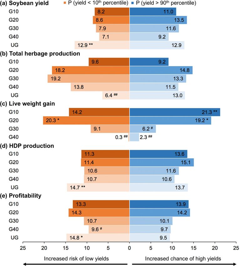
www.nature.com/scientificreports/
million ha currently cultivated with summer cash crops in the region (soybean, maize and rice), only 2.5 million
ha are rotated with winter cash crops and 2.2 million ha with off-season m aize25, while the rest often has winter
23
cover crops in no-till systems which could be grazed . Considering that this is the Brazilian region with the
highest levels of ICLS adoption (13% of the total area cultivated with crops is integrated with livestock)26, there
is a large unexplored potential for ICLS implementation. Implementing commercial-scale ICLS is a complex
challenge27 and concerns over the impact of livestock on subsequent crop yields and the greater managerial
intensity and knowledge demanded by ICLS have been listed as the main barriers to a doption23,28–30.
Various reports have reviewed the benefits and tradeoffs of crop-livestock integration for soil quality, nutrient
cycling, crop and animal production and farm economic performance in a wide range of systems and regions
of the world23,28–32. Livestock integration increases land-use efficiency and farm profitability while providing
opportunities to bolster ecological mechanisms underlying resilience33. Income diversification can reduce risks
from uncontrolled variability in climate and market fluctuations, as annual returns from crop and livestock
commodities are often uncorrelated28,34,35. At the field scale, self-regulating processes such as greater nutrient
cycling32, higher microbial functional d iversity36 and improved soil s tructure37 and organic m atter38 in grazed
systems are suggested to increase systems’ biophysical buffering capacity to less optimal environmental condi-
tions, in ways that still require better understanding14,37. Livestock production within ICLS also takes advantage
of crop residues and grasses inedible to humans to produce high-quality food (e.g., beef and milk byproducts),
thus reducing market competition for human-edible feed resources39. However, if we aim to use crop-livestock
integration as a tool for sustainable intensification, it is imperative to assess its contribution to not only system
productivity but also stability over the long-term.
Stability has multiple meanings in ecology and statistics and encompasses concepts like resistance and
resilience14,40–42. In this study, we considered the concept of stability as related to variability and defined a stable
system as one that changes least in response to environmental changes43. Management approaches that promote
biodiversity (e.g., organic agriculture and crop rotation diversity) and conservation practices (e.g., permanent soil
cover and reduced disturbance) have been shown to enhance yield stability13,15,22,42,44–53. Besides income diver-
sification, more biodiverse systems can stabilize agroecosystem productivity through cross-scale mechanisms
ranging from redundancy and facilitation in plant c ommunities41,53, to creating habitat for natural enemies to
promote pest suppression12. Conservation practices, in turn, can improve properties related to soil health and
crop yield stability, such as soil organic matter and water retention49,50. However, the effects of increasing system
diversity and ecological complexity by adding a trophic level (i.e., grazing animals) on the long-term stability of
no-till cropping systems have not yet been studied with the same level of detail.
The primary goal of this study was to evaluate long-term yields and stability of ICLS yields and profitability
compared to non-integrated systems under a range of environmental conditions and test their potential as a
strategy for sustainable intensification. We hypothesized that increased biodiversity and ecological complexity
created by crop-livestock integration in no-till systems improve yields while decreasing vulnerability of system
yields and profitability to weather variation. We tested this hypothesis using a 16-year dataset from a long-term,
no-till integrated soybean-beef cattle system in southern Brazil and measured the impacts of cover crop grazing
at different intensities during the winter period on probability of high and low performance13,15,44, minimum and
maximum yield potentials and stability of key crop, pasture, animal and whole-system outcomes using established
metrics of s tability22,44–50. Our results provide insight into the long-term stability of subtropical soybean systems
performance and the potential of livestock integration to build up sustainability and resilience in agriculture.
Methods
Site description and experimental design. The experiment was established at Espinilho Farm, in the
municipality of São Miguel das Missões, Rio Grande do Sul State, southern Brazil (28° 56′ 14″ S, 54° 20′ 52″ W,
465 m above sea level) in 2001. The region has a warm, humid subtropical climate (Cfa, Köppen classification
system) with an average annual temperature of 18.6 °C and average annual precipitation of 1898 mm54. Tempera-
ture and precipitation during the experimental period analyzed here (2001–2016) were collected by a weather
station located at the experimental site (Supplementary Fig. S1). Missing weather data points were estimated
using linear regression with values from the nearest meteorological station as predictor (National Institute of
Meteorology, Cruz Alta, 78 km from the study site 28° 36′ 12′′ S, 53° 40′ 25′′ W, 427 m a.s.l.). The soil in the
experimental site is an Oxisol (Rhodic Hapludox)55, with clayey texture (540, 270 and 190 g kg−1 of clay, silt and
sand, respectively) and a deep, well drained profile.
The area has been managed as no-till soybean [Glycine max (L.) Merr.] cropland since 1993. In 2001, 22
hectares of land began to be managed as an integrated soybean-beef cattle annual rotation with a mixture of
black oat (Avena strigosa Schreb.) and Italian ryegrass (Lolium multiflorum Lam.) pastures grazed during the
winter between soybean crops. Soybean was direct-seeded after the animals were removed from the experimental
area, typically in November, and harvested after 142 ± 11 days. After soybean harvest (April–May), experimental
plots were drill-seeded with black oats into the volunteer ryegrass sward from the previous winter, immediately
followed by broadcast seeding of ryegrass to ensure successful establishment for both species in all treatments.
The experiment was established as a randomized complete block design with three replicates. Treatments
consisted of four grazing intensities (intense, moderate, moderate-light and light) defined by contrasting sward
heights under continuous stocking (10, 20, 30 and 40 cm, respectively) and an ungrazed control with the same
pasture species used as winter cover crops. Plot areas were 0.1 ha for the ungrazed treatment and ranged from
0.8 to 3.6 ha for grazed treatments. Plots differed in area to reduce the number of animals required to maintain
the target treatment heights, especially for shorter swards.
Fertilization rates and soybean cultivars changed according to recommendations over the years but were the
same for all plots, including the ungrazed treatment. An average of 160 kg ha−1 urea (46% N) was applied yearly,
Scientific Reports | (2021) 11:1649 | https://doi.org/10.1038/s41598-021-81270-z 2
Vol:.(1234567890)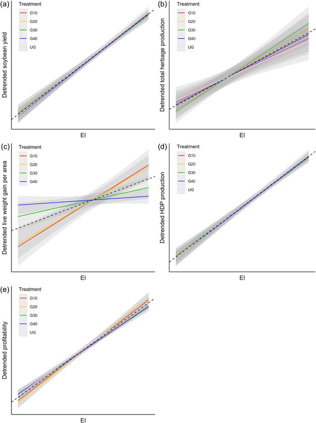
www.nature.com/scientificreports/
split into two equal winter applications during the stocking period: (1) when pasture reached V3–V4 growth
stage (i.e., plants with 3–4 fully expanded leaves on the main stem) and (2) just before animals entered the
experimental plots, approximately 1 month after the first application. From 2001 to 2011, P and K (on average,
60 kg ha−1 P2O5 and 70 kg ha−1 K2O) were applied at soybean sowing. From 2012 to 2016, P and K (on average,
45 kg ha−1 P2O5 and 60 kg ha−1 K2O) were applied at pasture sowing to take advantage of the improved nutrient
recycling provided by the grazing animals for primary production. The exact amount of fertilized applied each
year was based on standard recommendations56 and soil analysis.
Grazing usually started in June–July, when average sward height reached 24 ± 4 cm (or 1485 ± 379 kg ha−1 of
dry matter) and lasted 124 ± 16 days. To ensure that treatments remained close to their nominal targets (Supple-
mentary Fig. S2), sward height was measured at 100 random points per plot every 15 days with a sward stick57.
Three tester animals remained permanently in the plots over the stocking period and put-and-take animals
were added or removed to adjust sward h eights58. Average stocking rates used to maintain target sward heights
throughout the stocking period were 376, 651, 948 and 1331 kg of live weight ha−1 for light to intense grazing.
Experimental animals were crossbred Angus × Hereford × Nelore steers with initial body weight of 210 ± 23 kg
and 12 months of age on average. Steers were weighed at the beginning and at the end of the stocking period
after 12 h of fasting.
Long‑term data collection and variables studied. We assessed five key indicators of crop, pasture,
animal and whole-system performance: (1) soybean grain yield; (2) total herbage production; (3) animal live
weight gain; (4) human-digestible protein (HDP) production; and (5) profitability. “Year” in all analyses refers to
the year when soybeans were sown. To avoid bias, specific years were removed from the analysis when data for
one or more treatments were missing for a variable. Years 2001, 2003 and 2008 were excluded from the analyses
of soybean yield, protein production and income. Years 2001, 2004, 2005, 2006, 2007 and 2012 were excluded
from the analyses of herbage yield. Year 2012 was excluded from the analysis of animal production, protein
production and income.
Soybean yield (kg of grains h a−1) was determined at full grain maturity at 13% moisture content. Total herb-
age production (kg of dry matter ha−1) was calculated as the sum of pasture herbage mass on the first grazing
day and the daily herbage accumulation rates over the whole stocking period. Daily herbage accumulation rates
were estimated every 28 days using grazing exclusion cages59, following a standard protocol described by Nunes
et al.60. Steer live weight gain (kg of live weight h a−1) was calculated as the product of number of animals per
hectare, average daily gain (kg of live weight s teer−1 day−1) of the tester animals and number of grazing days of
the stocking period.
We adopted human-digestible protein (HDP) as a metric to account for added production from the livestock
component when comparing integrated to non-integrated systems. Livestock contributes to supplying human
protein demand as much or more than crop p roduction39,61 and do so by converting proteins from non-edible
(grass) into edible forms. HDP is not intended as a comprehensive nutritional analysis; rather, it is an unbiased
indicator of whole-system food p roduction62. Total HDP production (kg h a−1) was calculated as the sum of
protein from human-edible sources (i.e., animal and crop components of the system) multiplied by protein
digestibility of the products (beef and soybeans)61. We estimated the protein content of a 350 kg live weight steer
at the end of the stocking period as 19% of its body weight, based on National Research Council’s e quations63.
Soybean protein content was assumed to be 35% for a grain moisture content of 13%64.
We used gross profit (USD h a−1) as a metric of profitability, calculated as: (1) the difference between opera-
tional costs of soybean and cover crops and revenues from grain sales in the specialized system (Supplementary
Table S1); and (2) the difference between costs of soybean, cover crops and livestock operations (Supplementary
Table S2), opportunity cost of capital invested in beef cattle [calculated as the product of average stocking rate,
cattle price and saving account interest rate equivalent to the average number of grazing days (~ 2% interest rate)
according to the Central Bank of Brazil, Supplementary Table S2]65 and revenues from animal and grain sales in
the integrated crop-livestock systems. Revenues were calculated using yearly market sale prices of beef cattle and
soybean grains on November and April, respectively (Supplementary Table S3)66,67. Historic nominal prices were
transformed into real values using the General Market Price Index (IGP-M) from the Getúlio Vargas Foundation
(FGV), Brazil, using 2016 as the base year for the analysis68 and converted from Brazilian Reals (BRL) to U.S.
Dollars (USD) using the exchange rates of the respective months69. We used steer live weight gain to calculate
income from livestock, assuming similar price per unit mass of beef at purchase and sale. Annual costs of soybean
production were obtained from Brazil’s National Supply Company for the study region70. Soybean costs were
considered the same for all treatments, given similar crop management across experimental units. Annual costs
of cover crop establishment, animal medicines and mineral supplementation for the period of 2002–2011 were
obtained from the economic analysis done by Oliveira et al.33 in the same experimental protocol. For the period
of 2012–2016 costs were estimated using linear regression. Both costs and revenues were detrended prior to the
calculation of annual profits.
Statistical analysis. All statistical analyses were performed in R (version 3.6.1)71. Long-term crop, pasture,
animal and whole-system mean yields were analyzed using the lme4 package for mixed linear m odels72 with
treatments as fixed effects and years, blocks and plots within blocks as random effects (y ~ factor(year) * treat-
ment + (1|block/plot)). Yield trends over the 16 years were analyzed using linear mixed-effects models with
treatments and years as fixed effects and blocks and plots within blocks as random effects (y ~ year * treat-
ment + (1|block/plot)). Analysis of variance (ANOVA, Supplementary Tables S4 and S5) was performed and
when significant effects were detected, treatment means were compared with Tukey test at 95% confidence level
using the emmeans73 and lmerTest74 packages. Residuals of all analyses were visually checked for homogeneity
Scientific Reports | (2021) 11:1649 | https://doi.org/10.1038/s41598-021-81270-z 3
Vol.:(0123456789)www.nature.com/scientificreports/
of variance and normality was tested with quantile–quantile plots using the R car package75. When the residuals
were not homogeneous or the distribution was not normal, data were log or square root transformed as appro-
priate.
Yield stability analysis. We assessed stability of production (soybean yield, total herbage production, ani-
mal live weight gain, human-digestible protein) and profitability using four different metrics of stability: (1) yield
range, which is the maximum amplitude between minimum and maximum yield values in a time series44,45; (2)
coefficient of variation and (3) standard deviation21,44,45; and (4) Finlay and Wilkinson’s stability metric (FW)
derived from the linear regression of treatment yield on the mean yield of the location/year, or Environmental
Index (EI)44–49. Regression of detrended yield on EI, also called adaptability a nalysis47, can assess stability or
treatment-specific effect across a range of environments49. Based on regression of detrended yield on EI, stable
systems are those with smaller slope (less sensitive to changes in environment).
Yield range was calculated as the difference between the highest and the lowest yields for each variable over
the experimental period. Coefficient of variation, standard deviation and FW regressions were calculated using
detrended data. Detrending removed long-term linear trends potentially generated by treatments in order to only
consider variability of the residuals around the mean of each treatment due to transient environmental condi-
tions. Data were detrended by removing treatment effects and treatment-specific linear temporal trends using
the residuals of the linear model y ~ year * treatment. The overall average of the response variable was added to
the residuals to get intuitively more understandable values (addition of the same constant to all values does not
affect relevant statistical results).
Detrended data were analyzed as a function of the Environmental Index (EI) for each year and treatment
with the following model: detrended y ~ EI * treatment. EI was calculated as the average yield of all treatments
for each year, so that the highest and lowest EI indicated the year of highest and lowest system performance
respectively. FW regression slopes were calculated and compared using simultaneous general linear tests with
the R multcomp package76.
Yield range, coefficient of variation and standard deviation were analyzed as a function of treatment and
block (y ~ treatment + block) and when significant differences were detected, treatment means were compared
with Tukey test at 95% confidence level (⍺ = 0.05) using the R agricolae package77.
Treatments were ranked from the lowest (i.e., greatest stability, rank #1) to the highest value (i.e., lowest
stability, rank #5) for each stability metric regardless of the statistical significance. The overall stability of each
system output was ranked based on mean stability rank for the four stability metrics, such that treatments with
higher overall ranks indicated higher stability of yield or profitability.
Minimum and maximum yield potentials. Minimum and maximum yield potentials were calculated
based on predicted responses for the smallest and largest observed EI values for each studied indicator44,49,50.
Treatment effects on minimum and √ maximum yield potentials were tested with Tukey test at 95% confidence
level through the equation HSD = q 2SE , where HSD is Tukey’s honest significant difference, q is the studen-
tized range statistic obtained using the ‘qtukey’ function from R stats package71, and SE is the standard error of
the mean for the studied variable.
Downside risk and probability of high performance. To determine the probability of extreme yield
events over the given range of environmental conditions (EI), we modelled probability distributions of each
treatment’s detrended data using the ‘density’ function in R (Supplementary Code S1, adapted from Gaudin
et al.13). Treatment distributions were compared to a randomized distribution created by bootstrapping data
and ignoring treatment effects. Downside risk and probabilities of high performances were defined as estimated
probabilities of achieving results below the 10th percentile and above the 90th percentile, respectively, for each
of the studied indicators. 5000 randomizations were sufficient to stabilize the p values for every system output.
Treatment effects on the downside risk or probability of high performance were identified when observed results
were significantly different from the randomized distribution at the 95% confidence level beyond the determined
percentiles.
Results
Mean yields and trends. Soybean yields were not affected by winter grazing of cover crops, regardless
of the grazing intensity (p = 0.375, Table 1). Total herbage production increased with increasing sward height
(p < 0.001, Table 1) but remained low in the ungrazed treatment. Steers’ live weight gain per unit area increased
with grazing intensity (p < 0.001, Table 1). Addition of cattle to the system increased total human-digestible
protein production by up to 13% (p = 0.065, Table 1). Profitability in the two highest grazing intensities was 38%
greater than in the two lowest ones, and 112% greater than in the ungrazed treatment (p < 0.001, Table 1).
All variables, except for total herbage production, presented an increasing linear trend over time (Supple-
mentary Fig. S3, Supplementary Table S5). None of the linear trends were significantly affected by treatments, as
indicated by the absence of treatment by year interactions (Supplementary Table S5). When year was included
as a factor (categorical variable) in the model, there was a significant treatment by year interaction for total
herbage production and live weight gain (Supplementary Table S4). However, we were unable to detect a clear
pattern in the interactions.
Yield stability. Soybean yield was the most stable when the pasture phase was managed at moderate grazing
intensities (G20 and G30) according to the overall stability rank (Table 1). Ungrazed (UG) and lightly grazed
(G40) treatments were more sensitive to the environmental gradient than more intensively grazed treatments
Scientific Reports | (2021) 11:1649 | https://doi.org/10.1038/s41598-021-81270-z 4
Vol:.(1234567890)www.nature.com/scientificreports/
Indicator Treatment Mean yield Stability parameters Overall rank
Yield range Coefficient of variation (%) Standard deviation FW slope
G10 2882.58 4020.60 (3) 40 (3) 1157.72 (4) 0.99 (2) 3
G20 2857.27 3993.37 (2) 39 (2) 1127.47 (2) 0.98 (1) 1.8
Soybean yield (kg grain ha−1) G30 2835.15 4026.83 (4) 40 (3) 1115.64 (1) 0.98 (1) 2.3
G40 3086.35 4030.53 (5) 38 (1) 1157.51 (3) 1.02 (3) 3
UG 2974.50 3797.03 (1) 46 (4) 1279.53 (5) 1.04 (4) 3.5
G10 6493.02 b 5382.73 (2) 26 (3) 1678.63 (1) 0.87 (2) 2
G20 7447.46 ab 6445.77 (4) 28 (4) 2119.21 (4) 1.08 (4) 4
Total herbage production (kg DM ha−1) G30 7735.80 a 7023.67 (5) 29 (5) 2202.73 (5) 1.21 (5) 5
G40 8118.69 a 6074.67 (3) 24 (1) 1949.07 (3) 0.96 (3) 2.5
UG 6859.84 ab 5079.05 (1) 25 (2) 1733.51 (2) 0.81 (1) 1.5
G10 509.92 a 348.23 a (4) 18 (2) 93.75 a (4) 1.66 a (4) 3.5
G20 428.41 b 270.57 ab (3) 19 (3) 80.35 ab (3) 1.57 a (3) 3
Live weight gain (kg LW ha−1)
G30 310.83 c 212.27 ab (2) 18 (2) 56.23 bc (2) 0.59 b (2) 2
G40 183.16 d 135.67 b (1) 16 (1) 28.74 c (1) 0.18 b (1) 1
G10 780.55 1121.66 (5) 36 (1) 320.14 (4) 0.99 (2) 3
G20 765.09 1111.16 (4) 36 (1) 314.16 (3) 0.99 (2) 2.5
Human-digestible protein production (kg HDP ha−1) G30 720.54 1095.90 (3) 37 (2) 304.94 (1) 0.98 (1) 1.8
G40 749.94 1094.92 (2) 37 (2) 313.69 (2) 1.00 (3) 2.3
UG 692.29 1036.59 (1) 46 (3) 349.31 (5) 1.03 (4) 3.3
G10 940.25 a 1679.39 (4) 51 b (1) 509.27 (4) 1.06 (4) 3.3
G20 842.81 a 1849.11 (5) 57 b (2) 513.92 (5) 1.10 (5) 4.3
Profitability (USD ha−1) G30 691.24 b 1467.58 (1) 58 b (3) 435.60 (2) 0.94 (2) 2
G40 598.09 b 1475.99 (2) 66 b (4) 430.82 (1) 0.92 (1) 2
UG 419.84 c 1621.14 (3) 106 a (5) 490.09 (3) 0.98 (3) 3.5
Table 1. Mean yields and stability parameters of a long-term (2001–2016) soybean system integrated with
livestock at different grazing intensities or left ungrazed in the winter period. G10: intense grazing (10 cm
sward height); G20: moderate grazing (20 cm sward height); G30: moderate-light grazing (30 cm sward
height); G40: light grazing (40 cm sward height); UG: ungrazed cover crop. FW slope represents the Finlay and
Wilkinson regression slope. Numbers in parentheses rank the treatments for each variable within each column.
Different letters in the column represent significant differences among treatments according to the Tukey test
(⍺ = 0.05).
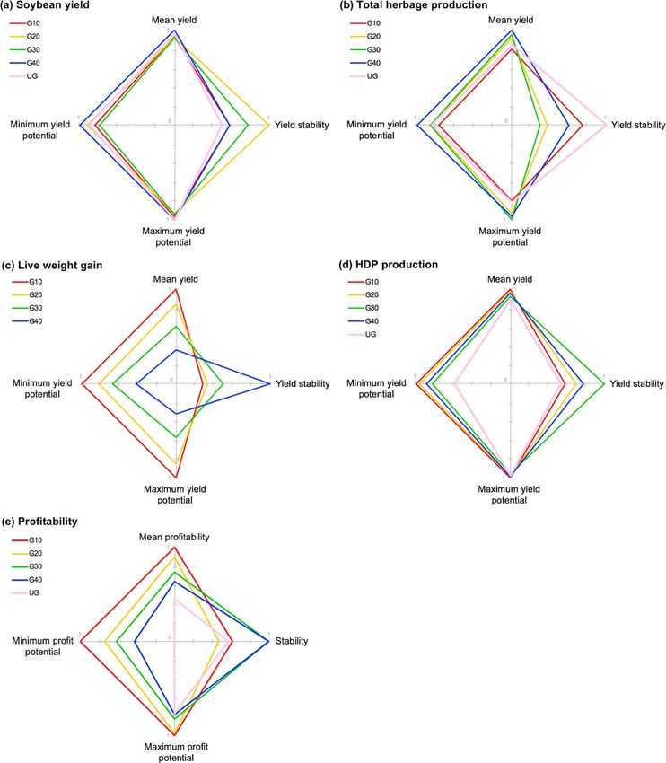
(FW slopes > 1, Fig. 1a, Table 1), indicating lower stability. The ungrazed treatment presented the narrowest yield
range but was ranked worst in all the other stability metrics, making it the least favorable to soybean yield stabil-
ity (Table 1). Intense (G10) and light grazing (G40) were similar and intermediate in overall stability.
Conversely, total herbage production was the least stable under moderate grazing intensities, with G30 and
G20 ranking fifth and fourth, respectively, in all stability metrics (Table 1). Both treatments were more respon-
sive to changes in Environmental Index (Fig. 1b). The UG control presented the most stable herbage production
over the years, ranking first in FW slopes and yield range, and second in CV and standard deviation, followed
by G10 and G40 (Table 1).
Increasing grazing intensity reduced the overall stability of live weight gain (Table 1). Light grazing (G40)
ranked first for all stability metrics for live weight gain and, along with G30, was significantly more stable than
G10 and G20 to the environmental gradient (p < 0.05, Fig. 1c, Table 1).
Both human-digestible protein (HDP) production and profitability showed greater stability when pastures
were grazed at moderate to light intensities (G30 and G40), while either over-intensification or the absence of
grazing decreased system stability (Table 1). The UG control had a 26% and 83% higher CV for HDP production
and profitability, respectively, than the grazed treatments and was the only stability metric showing statistical
significance for profitability (p < 0.05, Table 1). FW slopes for HDP production followed the same trends as
soybean yields, with greater slopes (> 1) for the G40 and UG treatments (Fig. 1d, Table 1). Profitability, in turn,
trended together with live weight gains, with lower FW slopes for G30 and G40 and greater slopes for G10 and
G20 (Fig. 1e, Table 1). Differently from live weight gains, however, G20 was less stable than G10 in all stability
metrics except for CV (Table 1). The combination of prices and live weight gains might have been the reason
why G10 and G20 switched positions in the profitability rank.
Downside risk and minimum yield potentials. The absence of grazing (UG) significantly (1) increased
the downside risk for soybean yield (⍺ = 0.01, Fig. 2a) without significantly impacting the minimum yield poten-
tial (Table 2); (2) increased risks of obtaining low HDP production (⍺ = 0.01, Fig. 2d); (3) increased risks of
financial loss (⍺ = 0.05, Fig. 2e); and (4) had the lowest minimum profitability (− 215.42 USD ha−1, p < 0.05,
Table 2). Both downside risk and minimum yield potential can be used as proxies of system resistance, since they
Scientific Reports | (2021) 11:1649 | https://doi.org/10.1038/s41598-021-81270-z 5
Vol.:(0123456789)www.nature.com/scientificreports/
Figure 1. Yield stability of (a) soybean yield (kg grain h
a−1), (b) total herbage production (kg dry matter ha−1),
(c) animal live weight (LW) gain (kg LW ha−1), (d) human-digestible protein (HDP) production (kg HDP ha−1)
and (e) profitability (USD ha−1) of soybean systems integrated with different levels of cattle grazing during the
winter period. Environmental index (EI) was calculated as the yearly mean detrended yield. Dashed lines are
the regression of detrended yields against the EI without treatment effects. G10: intense grazing (10 cm sward
height); G20: moderate grazing (20 cm sward height); G30: moderate-light grazing (30 cm sward height); G40:
light grazing (40 cm sward height); UG: ungrazed cover crop. Smaller slopes indicate greater yield stability.
Scientific Reports | (2021) 11:1649 | https://doi.org/10.1038/s41598-021-81270-z 6
Vol:.(1234567890)www.nature.com/scientificreports/
Figure 2. Effect of grazing intensity on the probability of obtaining high and low (a) soybean yield (kg grain
ha−1), (b) total herbage production (kg dry matter ha−1), (c) animal live weight (LW) gain (kg LW ha−1), (d)
human-digestible protein (HDP) production (kg HDP ha−1) and (e) profitability (USD ha−1) of soybean
systems integrated with different levels of cattle grazing during the winter period in southern Brazil. Shown are
the probabilities of yielding below the 10th percentile (orange bars) or above the 90th percentile (blue bars).
Statistically significant treatment effect was identified for higher probability of high/low yields at the 95% (*) or
99% (**) confidence level and for lower probability of high/low yields at the 95% (#) or 99% (##) confidence level.
G10: intense grazing (10 cm sward height); G20: moderate grazing (20 cm sward height); G30: moderate-light
grazing (30 cm sward height); G40: light grazing (40 cm sward height); UG: ungrazed cover crop.
represent the ability of a system to avoid crop failure or financial loss under stressful environmental conditions44.
That said, livestock integration increased system resistance to financial loss by 81% in the lightest grazing inten-
sity (G40) and up to 188% in the highest grazing intensity (G10) compared to the ungrazed control in the harsh-
est environmental conditions (p < 0.05, Table 2). Despite minimum HDP production not being significantly
different among treatments, it was 55% greater in grazed treatments compared to UG and up to 69% greater than
UG in the highest grazing intensity.
Conversely, UG presented a lower risk of low herbage production (⍺ = 0.01, Fig. 2b) despite no statistical dif-
ferences in minimum yield potential (Table 2). G20 and G30 had higher probability of low herbage production
(18 and 19%, respectively), but were not different from the random distribution (⍺ = 0.05, Fig. 2b). G20 prob-
ability of low live weight gain was significantly higher (⍺ = 0.05). G40 presented significantly lower downside
Scientific Reports | (2021) 11:1649 | https://doi.org/10.1038/s41598-021-81270-z 7
Vol.:(0123456789)www.nature.com/scientificreports/
Indicator Treatment Minimum yield potential Maximum yield potential
G10 509.43 4925.05
G20 558.09 4746.89
Soybean yield (kg grain ha−1) G30 479.18 4784.52
G40 605.47 5049.36
UG 548.67 5026.09
G10 4798.73 9271.93
G20 5347.92 10,891.05
Total herbage production (kg DM ha−1) G30 5396.34 11,572.91
G40 6252.24 11,179.98
UG 5287.69 9445.18
G10 399.79 a 593.43 a
G20 327.30 ab 507.20 a
Live weight gain per area (kg LW ha−1)
G30 270.06 b 338.66 b
G40 170.32 c 190.26 c
G10 234.54 1267.77
G20 225.82 1250.97
Human-digestible protein production (kg HDP ha−1) G30 193.21 1211.53
G40 207.71 1254.28
UG 139.02 1241.88
G10 189.04 a 1888.02 a
G20 84.62 ab 1845.45 ab
Profitability (USD ha-1) G30 35.57 ab 1559.39 bc
G40 − 40.40 b 1467.44 c
UG − 215.42 c 1447.02 c
Table 2. Minimum and maximum yield potentials of a long-term (2001–2016) soybean system integrated
with livestock at different grazing intensities or left ungrazed in the winter period. G10: intense grazing (10 cm
sward height); G20: moderate grazing (20 cm sward height); G30: moderate-light grazing (30 cm sward
height); G40: light grazing (40 cm sward height); UG: ungrazed cover crop. Different letters in the column
represent significant differences among treatments according to the Tukey test (⍺ = 0.05).
risk for live weight gain (⍺ = 0.01, Fig. 2c) but also a significantly lower minimum live weight gain potential
(⍺ = 0.05, Table 2).
Probability of high performance and maximum yield potentials. Treatment effect on the prob-
ability of high performance was larger for live weight gains than for the other variables. High (G10) and mod-
erate (G20) grazing intensities significantly increased the chance of obtaining live weight gains above the 90th
percentile (⍺ = 0.01 and ⍺ = 0.05, respectively, Fig. 2c). Conversely, moderate-light (G30) and light (G40) grazing
intensities reduced the chance of high live weight gains (⍺ = 0.05 and ⍺ = 0.01, respectively, Fig. 2c) and maxi-
mum yield potentials relative to G10 and G20 (Table 2).
We observed greater maximum profitability potential in G10 and G20 than in the UG control (1866.73 average
vs. 1447.02, a 29% increase, p < 0.05, Table 2), but probability of high performance was not affected (Fig. 2e). No
changes in probability of high performance were detected for soybean yield, total herbage production and HDP
production. Likewise, maximum yield potentials were not statistically different between treatments (Table 2),
despite the important difference in pasture dry matter production from G10 and UG to moderate to light graz-
ing intensities (G20, G30 and G40) that ranged from 1445.87 kg DM ha−1 (G20 vs. UG) to 2300.98 kg DM h a−1
(G30 vs. G10).
The most important findings of our study were: (1) grazing did not impair subsequent soybean yields regard-
less of grazing intensity, but moderate grazing intensities favored long-term yield stability (Fig. 3a); (2) herbage
production was more stable over the years but significantly lower under heavy grazing and in the absence of
grazing (Fig. 3b); (3) live weight gains were generally greater but less stable at higher grazing intensities (Fig. 3c);
(4) grazing at moderate to light intensities increased the stability of HDP production, while over-intensification
and absence of grazing increased system vulnerability to environmental oscillations (Fig. 3d); and (5) livestock
integration under lighter grazing intensities provided more stable profits over time, but risk of financial loss
reduced and overall system profitability increased with grazing intensity (Fig. 3e).
Discussion
Integrated crop-livestock systems (ICLS) are proposed as one possible strategy towards the sustainable intensi-
fication of food s ystems2,23,29,30. In a context of climate change and increased environmental pressure, stability of
agricultural systems performance—not just performance per se—needs to be evaluated to prioritize management
Scientific Reports | (2021) 11:1649 | https://doi.org/10.1038/s41598-021-81270-z 8
Vol:.(1234567890)www.nature.com/scientificreports/
Figure 3. Tradeoffs between performance and stability of (a) soybean yield (kg grain h a−1), (b) total herbage
production (kg dry matter ha−1), (c) animal live weight (LW) gain (kg LW ha−1), (d) human-digestible protein
(HDP) production (kg HDP h a−1) and (e) profitability (USD ha−1) of soybean systems integrated with different
levels of cattle grazing during the winter period in southern Brazil. Values represent standardized ratio to the
maximum value for each metric. Yield stability is the average rank of four stability metrics (Table 1).
strategies with the greatest adaptive gains. Mining data from long-term trials provides opportunities to compre-
hensively assess the performance and stability of key crop, pasture, animal and whole-system indicators when
livestock is integrated into specialized cropping systems.
Scientific Reports | (2021) 11:1649 | https://doi.org/10.1038/s41598-021-81270-z 9
Vol.:(0123456789)www.nature.com/scientificreports/
Grazing did not impair soybean grain yields regardless of grazing intensity, but moderate grazing intensities
favored soybean long-term yield stability (Fig. 3a). Our analysis of soybean yields supports previous studies
showing that grazing is not detrimental to crop productivity37,78,79. The impact of livestock on subsequent crop
yields has long been a concern, mainly due to potential soil compaction caused by animal trampling, consump-
tion of cover crop biomass and nutrient export when animals are removed from the system23,78. Results from
literature on ICLS have shown everything from decreases in subsequent crop y ield80, to no e ffect37,78,79 and even
increases23,30,81. In our systems, grazing is combined with low disturbance (i.e., no-till) which may help mitigate
potential negative impacts such as soil compaction. When conservation agricultural practices are used and graz-
ing is well-managed (i.e., assuming no overgrazing or abnormally wet years), effects on soil physical attributes
such as increased soil density have been shown to be transient, restricted to soil surface, and of limited impacts
on yields78.
Our study provides the first evidence of grazing-induced long-term yield stability in no-till soybean systems
where crops and livestock were integrated under moderate grazing intensity (Fig. 3a). Furthermore, our risk
analysis has shown that the absence of grazing increases the risk of yielding below the 10th percentile in unfa-
vorable years (Fig. 2a), despite greater litter amounts covering soil in ungrazed p lots60. The underlying processes
of increased yield stability with moderate grazing may be associated with increased biological diversity and eco-
logical interactions created by livestock integration. Properties associated with the maintenance of soil functions
and crop stability such as soil a ggregation32, microbial d iversity36,82 and ratios of beneficial over detrimental soil
82
nematodes were shown to be improved by moderate grazing in previous studies at this experimental site and
may have provided better growing conditions for the soybean crop in stressful years. Moderate grazing intensities
enhance root growth, exudation and turnover which, combined with manure deposition, can directly benefit
soil aggregation and microbial activity and diversity32. This in turn can lead to greater soil physical stabilization,
organic matter a ccumulation83,84 and nutrient c ycling84. These soil health benefits, including more biodiverse soil
communities, may be particularly relevant to maintain soil functioning under stress as shown in other s ystems85,86
and potential core mechanisms underlying crop yield stability.
Total herbage production increased with increasing sward height but remained low in the ungrazed treatment,
and was the least stable under moderate grazing intensities, demonstrating a possible trade-off between yield and
stability in forage crops (Fig. 3b). No grazing (UG) and heavy grazing (G10) treatments were more stable but
produced significantly less forage over the years (Table 1). Moderate grazing intensities created more responsive
forage growth to better environmental conditions and along with light grazing (G40) were able to produce ~ 11
tons DM h a−1, while G10 and UG reached less than 10 tons DM h a−1 even in the best environment (Table 2).
Lower stocking rates in G40 and UG favored the maintenance of target sward heights (and consequently leaf
area index) in dry years, so that daily herbage accumulation rates in these treatments were less affected by poor
environmental conditions. These results support long established plant–herbivore models87 and the existence of
two stable steady-states between vegetation growth and animal consumption in grazing lands: a low-productivity
stable equilibrium at low plant biomass (G10), and a high-productivity stable equilibrium at high plant biomass
(somewhere between G40 and UG). Moderate grazing (G20 and G30) provided a mid-range unstable state at
which pasture growth is high, but herbage mass and accumulation rates are more easily affected by disturbances
(e.g., weather fluctuations, fertilization or grazing itself), thus requiring more frequent adjustments of stocking
rate to keep sward heights close to the nominal targets87.
In the absence of grazing, forage yields presented a lower risk of low production in unfavorable years (Fig. 2).
Keeping a dense layer of residual biomass on the soil surface in no-till systems (during winter as cover crop/
pasture and after winter, as straw) improves soil water retention37 and protects soil from e rosion88 and weed
outbreak89 with potential benefits to crops in rotation. For this reason, crop-livestock integration is seen by many
farmers as detrimental to no-till systems. However, prior research at this site showed no direct impacts of greater
litter mass on crop yields in the ungrazed system37. On the other hand, the greater herbage production under
moderate to light grazing intensities and the reduced probability of low forage yields in the ungrazed system
found in our study may help explain the increased soil carbon stocks found by previous authors in areas man-
aged under these approaches compared to intensely grazed areas after a decade of crop-livestock integration at
this site38. Previous studies in humid continental climate of the US have shown that agronomic practices able to
increase soil water holding capacity and organic matter can buffer yield volatility of rainfed maize49, suggesting
that our results may apply to different agroecosystems around the world.
The linear increase of live weight gains per unit area (Table 1) with grazing intensity is consistent with previ-
ous studies and can be attributed to increased stocking rate required to keep pasture at target sward h eights90.
Constraints in animal dry matter intake when forage allowances are limiting could result in a quadratic response
of live weight gain, with greater gains associated with moderate grazing intensities91,92. The shortest sward height
used in our study in fact limits the intake93 and consequently the individual live weight gains90,93, but it was not
restrictive enough to show the quadratic pattern when results were expressed on a per area basis because greater
stocking rate compensated the decrease in individual performance.
Our analysis showed a clear trade-off between yields and stability of live weight gains (Fig. 3c). Live weight
gains were generally greater, but less stable at higher grazing intensities. Although pasture growth is less stable and
requires more frequent stocking rate adjustments under moderate grazing intensities, more intense stocking rate
adjustments are required at the extremities of the grazing intensity gradient. In other words, the closer to a stable
state, the stronger the push (i.e., addition or removal of animals) in the opposite direction required to shift states
will be87. In our case, this was translated as a strong removal of animals from the plots when swards got too short
to allow pasture regrowth in higher grazing intensities, which probably resulted in less stable live weight gains.
Besides being less stable, literature also shows that higher grazing intensities lead to greater greenhouse gas emis-
sions, especially m ethane93. Thus, to sustainably intensify ICLS, a ‘conciliatory stocking rate’90,94 able to achieve
high animal yields and overall system stability while keeping low environmental footprint should be pursued.
Scientific Reports | (2021) 11:1649 | https://doi.org/10.1038/s41598-021-81270-z 10
Vol:.(1234567890)www.nature.com/scientificreports/
Intensification of ruminant production in the last decades has increased protein production per area of land
use, but primarily as a result of increased use of feed concentrates and human-edible nutrients in developed
countries10,39. However, addressing the ability of a system to sustainably increase food production must consider
the quality of food produced for human nutrition as well as the ability of this system to produce food from
human inedible resources39. Grazing at moderate to light intensities increased HDP production and stability,
while over-intensification and absence of grazing increased system vulnerability to environmental oscillations
(Fig. 3d). Ungrazed cover crops represented a risk to food production in unfavorable years (Fig. 2d), since low
soybean protein yields are not buffered by livestock protein yields as in integrated systems. By comprising protein
from both crop and animal components of the system, our HDP analysis can be used as a measure of land-use
efficiency61. Despite lacking statistical significance, grazing improved land-use efficiency by up to 13% due to
the contribution of grass-based beef, an animal-derived protein of higher quality in human nutrition metrics
than plant derived p roteins39.
The greater profitability of integrated systems, particularly in heavier grazing intensities (G10 and G20, Fig. 3e,
Table 1), was similar to results from a previous study at this s ite33 but differs in the magnitude of the results. While
we observed profits 38% greater in the two highest grazing intensities (G10 and G20) compared to the two lowest
ones (G30 and G40), and 112% greater than in UG treatment, Oliveira et al.33 found 27% and 100% increases
(averages of 669, 526 and 334 USD h a−1, respectively). This difference might be explained by international meat
prices, which raised steadily during the period comprised by their study (2001–2011) and remained relatively
stable at a higher level after that95. Furthermore, two major droughts occurred during their study period and
severely affected soybean yields and profitability of the systems. Moreover, soybean yields kept trending upwards
from 2011 to 2016 (Supplementary Fig. S3). Another possible explanation is that those authors used the nominal
purchase and sale prices practiced by the farmer at every beginning and end of stocking seasons, which might
have led to lower profits because purchase prices per kg of yearling steers are usually higher than sale prices of
steers at the end of the fattening period. Although one could argue that their method is more realistic than ours,
we consider our method more reliable because it disregards potential benefits or disadvantages faced by the
farmer when trading the animals over the years.
The decrease in stability of whole-system profits with the over-intensification or the absence of grazing was
consistent with HDP production, with G30 and G40 being the most stable treatments (Fig. 3e, Table 1). However,
while stability of HDP production was the lowest in the absence of grazing (UG), profits were less stable in G20
followed by UG and G10 according to the overall rank (Table 1). Considering our ranking criterion, this outcome
was a result of G10 and G20 ranking 4th and 5th in every stability metric except for CV, in which they ranked
1st and 2nd (Table 1). The difference of CV to the other metrics is that it brings information of the variability
relative to the mean. Therefore, according to the CV, livestock integration reduced the variability relative to the
mean profit compared to UG regardless of grazing intensity, but when it comes to pure variability G10 and G20
were the least stable treatments.
These results countered our expectation that stability of profits would increase with stocking density, since
literature suggests crops and livestock markets are uncorrelated, which would work as a buffer against climate and
price fluctuations28,34. However, our results arise within the positively correlated beef cattle and soybean market
prices in Rio Grande do Sul State during the experimental period (r = 0.44, 95% confidence interval = 0.30–0.56,
p < 0.001, Supplementary Fig. S4a). Brazilian market prices of soybeans and cattle were also highly correlated in
the last 2 decades (r = 0.88, 95% confidence interval = 0.87–0.88, p < 0.001, Supplementary Fig. S4b)96,97. Thus,
while extra income from livestock might have buffered profit oscilations in G30 an G40 compared to UG (mainly
through increasing system resistance in less optimal environments, Table 2), outstanding system performance
in optimal environmental conditions (see maximum yield potential, Table 2) increased regression slopes and
interannual variability in G10 and G20, resulting in the lower stability observed for these treatments (Table 1).
Furthermore, the significantly higher risk of yielding below the 10th percentile (Fig. 2e) and the lower minimum
profitability potential in UG (Table 2) represent a riskier farm portfolio, while animal production in grazed treat-
ments provide a mean to smoothing farm incomes in poor crop production years (Table 2). These findings high-
light the importance of using multiple metrics for studies associating system performance and long-term stability.
In conclusion, our data suggest that livestock integration into specialized soybean systems under moderate to
light grazing intensities benefits whole system stability to environmental variability and confirm that grazing does
not impair subsequent soybean yields in annual soybean-pasture rotations. Instead, it reduces the chance of crop
failure in unfavorable years. Moreover, while livestock integration under lighter grazing intensities provides more
stable profits over time, economic risk reduction and overall system profitability increase with grazing intensity,
showing that probability and nature of win–win outcomes is a matter of management. Our results likely apply to
other ICLS designs, but best pasture management remains paramount to achieve benefits and reduce potential
tradeoffs. Our study also highlights the importance of long-term experimental protocols to understand complex
temporal system responses such as yield stability and improve predictions and adaptation to climate change.
Questions remain regarding what mechanisms are driving these results, especially for grazing-induced soybean
yield stability, but intensification of ecological processes likely plays a pivotal role.
Data availability
The datasets generated during and/or analyzed during the current study are available from the corresponding
author on reasonable request.
Received: 12 June 2020; Accepted: 5 January 2021
Scientific Reports | (2021) 11:1649 | https://doi.org/10.1038/s41598-021-81270-z 11
Vol.:(0123456789)www.nature.com/scientificreports/
References
1. Devendra, C. & Thomas, D. Smallholder farming systems in Asia. Agric. Syst. 71, 17–25 (2002).
2. Herrero, M. et al. Smart investments in sustainable food production: revisiting mixed crop-livestock systems. Science 327, 822–825
(2010).
3. Wright, I. A. et al. Integrating crops and livestock in subtropical agricultural systems. J. Sci. Food Agric. 92, 1010–1015 (2011).
4. Halstead, P. Pastoralism or household herding? Problems of scale and specialization in early Greek animal husbandry. World
Archaeol. 28, 20–42 (1996).
5. Bogaard, A. et al. Crop manuring and intensive land management by Europe’s first farmers. Proc. Natl. Acad. Sci. 110, 12589–12594
(2013).
6. Altieri, M. A., Nicholls, C. I., Henao, A. & Lana, M. A. Agroecology and the design of climate change-resilient farming systems.
Agron. Sustain. Dev. 35, 869–890 (2015).
7. Garrett, R. D. et al. Drivers of decoupling and recoupling of crop and livestock systems at farm and territorial scales. Ecol. Soc. 25,
24 (2020).
8. Verhoeven, J. T. A., Arheimer, B., Yin, C. & Hefting, M. M. Regional and global concerns over wetlands and water quality. Trends
Ecol. Evol. 21, 96–103 (2006).
9. Liu, J. et al. A high-resolution assessment on global nitrogen flows in cropland. Proc. Natl. Acad. Sci. 107, 8035–8040 (2010).
10. Macdonald, J. M., & Mcbride, W. D. The transformation of U.S. livestock agriculture: scale, efficiency, and risks (2009).
11. Gerber, P. J. et al. Tackling climate change through livestock: a global assessment of emissions and mitigation opportunities. Food
and Agriculture Organization of the United Nations (2013).
12. Lin, B. B. Resilience in agriculture through crop diversification: adaptive management for environmental change. Bioscience 61,
183–193 (2011).
13. Gaudin, A. C. M. et al. Increasing crop diversity mitigates weather variations and improves yield stability. PLoS ONE 10, e0113261
(2015).
14. Peterson, C. A., Eviner, V. T. & Gaudin, A. C. M. Ways forward for resilience research in agroecosystems. Agric. Syst. 162, 19–27
(2018).
15. Bowles, T. M. et al. Long-term evidence shows that crop-rotation diversification increases agricultural resilience to adverse growing
conditions in North America. One Earth 2, 284–293 (2020).
16. Lobell, D. B. & Field, C. B. Global scale climate-crop yield relationships and the impacts of recent warming. Environ. Res. Lett. 2,
014002 (2007).
17. Gornall, J. et al. Implications of climate change for agricultural productivity in the early twenty-first century. Philos. Trans. R. Soc.
B 365, 2973–2989 (2010).
18. Osborne, T. M. & Wheeler, T. R. Evidence for a climate signal in trends of global crop yield variability over the past 50 years.
Environ. Res. Lett. 8, 024001 (2013).
19. United Nations. Population division of the department of economic and social affairs of the United Nations: world population
prospects. https://population.un.org/wpp/DataQuery/ (2019).
20. Schmidhuber, J. & Tubiello, F. N. Global food security under climate change. Proc. Natl. Acad. Sci. 104, 19703–19708 (2007).
21. Bullock, J. M. et al. Resilience and food security: rethinking an ecological concept. J. Ecol. 105, 880–884 (2017).
22. Knapp, S. & van der Heijden, M. G. A. A global meta-analysis of yield stability in organic and conservation agriculture. Nat. Com-
mun. 9, 1–9 (2018).
23. de Moraes, A. et al. Integrated crop-livestock systems in the Brazilian subtropics. Eur. J. Agron. 57, 4–9 (2014).
24. Niles, M. T., Garrett, R. D. & Walsh, D. Ecological and economic benefits of integrating sheep into viticulture production. Agron.
Sustain. Dev. 38, 1–11 (2018).
25. Companhia Nacional de Abastecimento (CONAB). Safra brasileira de grãos: Tabela de levantamento. https://www.conab.gov.br/
info-agro/safras/graos (2020).
26. Empresa Brasileira de Pesquisa Agropecuária (Embrapa). ILPF em números. https://ainfo.cnptia.embrapa.br/digital/bitstream/
item/158636/1/2016-cpamt-ilpf-em-numeros.pdf (2016).
27. Garrett, R. D. et al. Social and ecological analysis of commercial integrated crop livestock systems: current knowledge and remain-
ing uncertainty. Agric. Syst. 155, 136–146 (2017).
28. Bell, L. W. & Moore, A. D. Integrated crop-livestock systems in Australian agriculture: trends, drivers and implications. Agric. Syst.
111, 1–12 (2012).
29. Sulc, R. M. & Franzluebbers, A. J. Exploring integrated crop-livestock systems in different ecoregions of the United States. Eur. J.
Agron. 57, 21–30 (2014).
30. Carvalho, P. C. F. et al. Animal production and soil characteristics from integrated crop-livestock systems: toward sustainable
intensification. J. Anim. Sci. 96, 3513–3525 (2018).
31. Russelle, M. P., Entz, M. H. & Franzluebbers, A. J. Reconsidering integrated crop-livestock systems in North America. Agron. J.
99, 325–334 (2007).
32. Carvalho, P. C. F. et al. Managing grazing animals to achieve nutrient cycling and soil improvement in no-till integrated systems.
Nutr. Cycl. Agroecosyst. 88, 259–273 (2010).
33. Oliveira, C. A. O. et al. Comparison of an integrated crop-livestock system with soybean only: economic and production responses
in southern Brazil. Renew. Agric. Food Syst. 29, 230–238 (2013).
34. Ryschawy, J., Choisis, N., Choisis, J. P., Joannon, A. & Gibon, A. Mixed crop-livestock systems: an economic and environmental-
friendly way of farming?. Animal 6, 1722–1730 (2012).
35. Peterson, C. A., Bell, L. W., Carvalho, P. C. F. & Gaudin, A. C. M. Resilience of an integrated crop–livestock system to climate
change: a simulation analysis of cover crop grazing in southern Brazil. Front. Sustain. Food Syst. 4, 604099 (2020).
36. Chávez, L. F. et al. Diversidade metabólica e atividade microbiana no solo em sistema de integração lavoura-pecuária sob inten-
sidades de pastejo. Pesq. Agropec. Bras. 46, 1254–1261 (2011).
37. Peterson, C. A. et al. Winter grazing does not affect soybean yield despite lower soil water content in a subtropical crop-livestock
system. Agron. Sustain. Dev. 39, 26 (2019).
38. Assmann, J. M. et al. Soil carbon and nitrogen stocks and fractions in a long-term integrated crop-livestock system under no-tillage
in southern Brazil. Agric. Ecosyst. Environ. 190, 52–59 (2014).
39. Peyraud, J. L. & Peeters, A. The role of grassland based production system in the protein security. Grassland Science in Europe - The
multiple roles of grassland in the European bioeconomy 21, 29–43 (2016).
40. Harrison, G. W. Stability under environmental stress: resistance, resilience, persistence, and variability. Am. Nat. 113, 659–669
(1979).
41. Lehman, C. L. & Tilman, D. Biodiversity, stability, and productivity in competitive communities. Am. Nat. 156, 534–552 (2000).
42. Isbell, F. et al. Biodiversity increases the resistance of ecosystem productivity to climate extremes. Nature 526, 574–577 (2015).
43. Lightfoot, C. W. F., Dear, K. B. G. & Mead, R. Intercropping sorghum with cowpea in dryland farming systems in Botswana. II.
Comparative stability of alternative cropping systems. Exp. Agric. 23, 435–442 (1987).
44. Li, M., Peterson, C. A., Tautges, N. E., Scow, K. M. & Gaudin, A. C. M. Yields and resilience outcomes of organic, cover crop, and
conventional practices in a Mediterranean climate. Sci. Rep. 9, 12283 (2019).
Scientific Reports | (2021) 11:1649 | https://doi.org/10.1038/s41598-021-81270-z 12
Vol:.(1234567890)You can also read