Local Explanations via Necessity and Sufficiency: Unifying Theory and Practice - PhilArchive
←
→
Page content transcription
If your browser does not render page correctly, please read the page content below
Local Explanations via Necessity and Sufficiency:
                                                                            Unifying Theory and Practice

                                                  David S. Watson*1                 Limor Gultchin*2,3                Ankur Taly4                Luciano Floridi5,3

                                                      *
                                                          Equal contribution 1 Department of Statistical Science, University College London, London, UK
                                                                      2
                                                                        Department of Computer Science, University of Oxford, Oxford, UK
                                                                  3
                                                                    The Alan Turing Institute, London, UK 4 Google Inc., Mountain View, USA
arXiv:2103.14651v2 [cs.LG] 10 Jun 2021

                                                                           5
                                                                             Oxford Internet Institute, University of Oxford, Oxford, UK

                                                                    Abstract

                                             Necessity and sufficiency are the building blocks
                                             of all successful explanations. Yet despite their im-
                                             portance, these notions have been conceptually un-
                                             derdeveloped and inconsistently applied in explain-
                                             able artificial intelligence (XAI), a fast-growing re-
                                             search area that is so far lacking in firm theoretical
                                             foundations. Building on work in logic, probabil-
                                             ity, and causality, we establish the central role of
                                             necessity and sufficiency in XAI, unifying seem-
                                             ingly disparate methods in a single formal frame-
                                             work. We provide a sound and complete algorithm
                                                                                                              Figure 1: We describe minimal sufficient factors (here, sets
                                             for computing explanatory factors with respect to
                                                                                                              of features) for a given input (top row), with the aim of
                                             a given context, and demonstrate its flexibility and
                                                                                                              preserving or flipping the original prediction. We report a
                                             competitive performance against state of the art al-
                                                                                                              sufficiency score for each set and a cumulative necessity
                                             ternatives on various tasks.
                                                                                                              score for all sets, indicating the proportion of paths towards
                                                                                                              the outcome that are covered by the explanation. Feature
                                         1   INTRODUCTION                                                     colors indicate source of feature values (input or reference).

                                         Machine learning algorithms are increasingly used in a va-           dard in many XAI applications, due in no small part to their
                                         riety of high-stakes domains, from credit scoring to medi-           attractive theoretical properties [Bhatt et al., 2020]. How-
                                         cal diagnosis. However, many such methods are opaque, in             ever, ambiguities regarding the underlying assumptions of
                                         that humans cannot understand the reasoning behind partic-           the method [Kumar et al., 2020] and the recent prolifera-
                                         ular predictions. Post-hoc, model-agnostic local explanation         tion of mutually incompatible implementations [Sundarara-
                                         tools (e.g., feature attributions, rule lists, and counterfactu-     jan and Najmi, 2019; Merrick and Taly, 2020] have com-
                                         als) are at the forefront of a fast-growing area of research         plicated this picture. Despite the abundance of alternative
                                         variously referred to as interpretable machine learning or           XAI tools [Molnar, 2021], a dearth of theory persists. This
                                         explainable artificial intelligence (XAI).                           has led some to conclude that the goals of XAI are under-
                                                                                                              specified [Lipton, 2018], and even that post-hoc methods do
                                         Many authors have pointed out the inconsistencies between
                                                                                                              more harm than good [Rudin, 2019].
                                         popular XAI tools, raising questions as to which method
                                         is more reliable in particular cases [Mothilal et al., 2020a;        We argue that this lacuna at the heart of XAI should be filled
                                         Ramon et al., 2020; Fernández-Loría et al., 2020]. Theoret-          by a return to fundamentals – specifically, to necessity and
                                         ical foundations have proven elusive in this area, perhaps           sufficiency. As the building blocks of all successful expla-
                                         due to the perceived subjectivity inherent to notions such           nations, these dual concepts deserve a privileged position
                                         as “intelligible” and “relevant” [Watson and Floridi, 2020].         in the theory and practice of XAI. Following a review of re-
                                         Practitioners often seek refuge in the axiomatic guarantees          lated work (Sect. 2), we operationalize this insight with a
                                         of Shapley values, which have become the de facto stan-              unified framework (Sect. 3) that reveals unexpected affinities

                                                                 Accepted for the 37th Conference on Uncertainty in Artificial Intelligence (UAI 2021).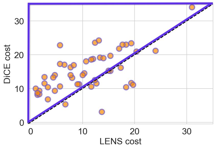
between various XAI tools and probabilities of causation          and Y = y 0 .” Then, according to Pearl [2000, Ch. 9], the
(Sect. 4). We proceed to implement a novel procedure for          probability that x is a sufficient cause of y is given by
computing model explanations that improves upon the state         suf(x, y) := P (yx |x0 , y 0 ), and the probability that x is a
of the art in various quantitative and qualitative comparisons    necessary cause of y is given by nec(x, y) := P (yx0 0 |x, y).
(Sect. 5). Following a brief discussion (Sect. 6), we conclude
                                                                  Analysis becomes more difficult in higher dimensions,
with a summary and directions for future work (Sect. 7).
                                                                  where variables may interact to block or unblock causal path-
We make three main contributions. (1) We present a formal         ways. VanderWeele and Robins [2008] analyze sufficient
framework for XAI that unifies several popular approaches,        causal interactions in the potential outcomes framework,
including feature attributions, rule lists, and counterfactu-     refining notions of synergism without monotonicity con-
als. (2) We introduce novel measures of necessity and suf-        straints. In a subsequent paper, VanderWeele and Richard-
ficiency that can be computed for any feature subset. The         son [2012] study the irreducibility and singularity of interac-
method enables users to incorporate domain knowledge,             tions in sufficient-component cause models. Halpern [2016]
search various subspaces, and select a utility-maximizing         devotes an entire monograph to the subject, providing vari-
explanation. (3) We present a sound and complete algorithm        ous criteria to distinguish between subtly different notions
for identifying explanatory factors, and illustrate its perfor-   of “actual causality”, as well as “but-for” (similar to nec-
mance on a range of tasks.                                        essary) and sufficient causes. These authors generally limit
                                                                  their analyses to Boolean systems with convenient structural
                                                                  properties, e.g. conditional ignorability and the stable unit
2   NECESSITY AND SUFFICIENCY                                     treatment value assumption [Imbens and Rubin, 2015]. Op-
                                                                  erationalizing their theories in a practical method without
Necessity and sufficiency have a long philosophical tradi-        such restrictions is one of our primary contributions.
tion [Mackie, 1965; Lewis, 1973; Halpern and Pearl, 2005b],       Necessity and sufficiency have begun to receive explicit at-
spanning logical, probabilistic, and causal variants. In propo-   tention in the XAI literature. Ribeiro et al. [2018a] propose
sitional logic, we say that x is a sufficient condition for y     a bandit procedure for identifying a minimal set of Boolean
iff x → y, and x is a necessary condition for y iff y → x.        conditions that entails a predictive outcome (more on this in
So stated, necessity and sufficiency are logically converse.      Sect. 4). Dhurandhar et al. [2018] propose an autoencoder
However, by the law of contraposition, both definitions ad-       for learning pertinent negatives and positives, i.e. features
mit alternative formulations, whereby sufficiency may be          whose presence or absence is decisive for a given label,
rewritten as ¬y → ¬x and necessity as ¬x → ¬y. By pair-           while Zhang et al. [2018] develop a technique for generat-
ing the original definition of sufficiency with the latter def-   ing symbolic corrections to alter model outputs. Both meth-
inition of necessity (and vice versa), we find that the two       ods are optimized for neural networks, unlike the model-
concepts are also logically inverse.                              agnostic approach we develop here.
These formulae suggest probabilistic relaxations, measur-         Another strand of research in this area is rooted in logic pro-
ing x’s sufficiency for y by P (y|x) and x’s necessity for y      gramming. Several authors have sought to reframe XAI as
by P (x|y). Because there is no probabilistic law of contra-      either a SAT [Ignatiev et al., 2019; Narodytska et al., 2019]
position, these quantities are generally uninformative w.r.t.     or a set cover problem [Lakkaraju et al., 2019; Grover et al.,
P (¬x|¬y) and P (¬y|¬x), which may be of independent              2019], typically deriving approximate solutions on a pre-
interest. Thus, while necessity is both the converse and in-      specified subspace to ensure computability in polynomial
verse of sufficiency in propositional logic, the two formula-     time. We adopt a different strategy that prioritizes complete-
tions come apart in probability calculus. We revisit the dis-     ness over efficiency, an approach we show to be feasible in
tinction between probabilistic conversion and inversion in        moderate dimensions (see Sect. 6 for a discussion).
Rmk. 1 and Sect. 4.
                                                                  Mothilal et al. [2020a] build on Halpern [2016]’s definitions
These definitions struggle to track our intuitions when we        of necessity and sufficiency to critique popular XAI tools,
consider causal explanations [Pearl, 2000; Tian and Pearl,        proposing a new feature attribution measure with some pur-
2000]. It may make sense to say in logic that if x is a neces-    ported advantages. Their method relies on the strong as-
sary condition for y, then y is a sufficient condition for x;     sumption that predictors are mutually independent. Galho-
it does not follow that if x is a necessary cause of y, then y    tra et al. [2021] adapt Pearl [2000]’s probabilities of cau-
is a sufficient cause of x. We may amend both concepts us-        sation for XAI under a more inclusive range of data gen-
ing counterfactual probabilities – e.g., the probability that     erating processes. They derive analytic bounds on multidi-
Alice would still have a headache if she had not taken an as-     mensional extensions of nec and suf, as well as an algo-
pirin, given that she does not have a headache and did take       rithm for point identification when graphical structure per-
an aspirin. Let P (yx |x0 , y 0 ) denote such a quantity, to be   mits. Oddly, they claim that non-causal applications of ne-
read as “the probability that Y would equal y under an in-        cessity and sufficiency are somehow “incorrect and mislead-
tervention that sets X to x, given that we observe X = x0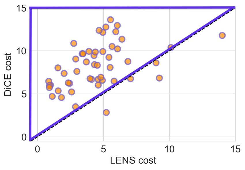
ing” (p. 2), a normative judgment that is inconsistent with      Factors. Factors pick out the properties whose necessity
many common uses of these concepts.                              and sufficiency we wish to quantify. Formally, a factor
                                                                 c : Z 7→ {0, 1} indicates whether its argument satisfies
Rather than insisting on any particular interpretation of ne-
                                                                 some criteria with respect to predictors or auxiliaries. For
cessity and sufficiency, we propose a general framework that
                                                                 instance, if x is an input to a credit lending model, and w
admits logical, probabilistic, and causal interpretations as
                                                                 contains information about the subspace from which data
special cases. Whereas previous works evaluate individual
                                                                 were sampled, then a factor could be c(z) = 1[x[gender =
predictors, we focus on feature subsets, allowing us to detect
                                                                 “female”] ∧ w[do(income > $50k)]], i.e. checking if z is
and quantify interaction effects. Our formal results clarify
                                                                 female and drawn from a context in which an intervention
the relationship between existing XAI methods and proba-
                                                                 fixes income at greater than $50k. We use the term “factor”
bilities of causation, while our empirical results demonstrate
                                                                 as opposed to “condition” or “cause” to suggest an inclusive
their applicability to a wide array of tasks and datasets.
                                                                 set of criteria that may apply to predictors x and/or auxil-
                                                                 iaries w. Such criteria are always observational w.r.t. z but
                                                                 may be interventional or counterfactual w.r.t. x. We assume
3   A UNIFYING FRAMEWORK                                         a finite space of factors C.

We propose a unifying framework that highlights the role of      Partial order. When multiple factors pass a given neces-
necessity and sufficiency in XAI. Its constituent elements       sity or sufficiency threshold, users will tend to prefer some
are described below.                                             over others. For instance, factors with fewer conditions are
                                                                 often preferable to those with more, all else being equal;
Target function. Post-hoc explainability methods assume
                                                                 factors that change a variable by one unit as opposed to two
access to a target function f : X 7→ Y, i.e. the model whose
                                                                 are preferable, and so on. Rather than formalize this pref-
prediction(s) we seek to explain. For simplicity, we restrict
                                                                 erence in terms of a distance metric, which unnecessarily
attention to the binary setting, with Y ∈ {0, 1}. Multi-class
                                                                 constrains the solution space, we treat the partial ordering
extensions are straightforward, while continuous outcomes
                                                                 as primitive and require only that it be complete and transi-
may be accommodated via discretization. Though this in-
                                                                 tive. This covers not just distance-based measures but also
evitably involves some information loss, we follow authors
                                                                 more idiosyncratic orderings that are unique to individual
in the contrastivist tradition in arguing that, even for con-
                                                                 agents. Ordinal preferences may be represented by cardi-
tinuous outcomes, explanations always involve a juxtapo-
                                                                 nal utility functions under reasonable assumptions (see, e.g.,
sition (perhaps implicit) of “fact and foil” [Lipton, 1990].
                                                                 [von Neumann and Morgenstern, 1944]).
For instance, a loan applicant is probably less interested in
knowing why her credit score is precisely y than she is in       We are now ready to formally specify our framework.
discovering why it is below some threshold (say, 700). Of
                                                                 Definition 1 (Basis). A basis for computing necessary and
course, binary outcomes can approximate continuous values
                                                                 sufficient factors for model predictions is a tuple B =
with arbitrary precision over repeated trials.
                                                                 hf, D, C, i, where f is a target function, D is a context, C
                                                                 is a set of factors, and  is a partial ordering on C.
Context. The context D is a probability distribution over
which we quantify sufficiency and necessity. Contexts may        3.1   EXPLANATORY MEASURES
be constructed in various ways but always consist of at least
some input (point or space) and reference (point or space).      For some fixed basis B = hf, D, C, i, we define the fol-
For instance, we may want to compare xi with all other           lowing measures of sufficiency and necessity, with probabil-
samples, or else just those perturbed along one or two axes,     ity taken over D.
perhaps based on some conditioning event(s).
                                                                 Definition 2 (Probability of Sufficiency). The probability
In addition to predictors and outcomes, we optionally in-        that c is a sufficient factor for outcome y is given by:
clude information exogenous to f . For instance, if any
events were conditioned upon to generate a given refer-                     P S(c, y) := P (f (z) = y | c(z) = 1).
ence sample, this information may be recorded among a            The probability that factor set C = {c1 , . . . , ck } is sufficient
set of auxiliary variables W . Other examples of potential       for y is given by:
auxiliaries include metadata or engineered features such as
those learned via neural embeddings. This augmentation al-                                                k
                                                                                                          X
lows us to evaluate the necessity and sufficiency of factors             P S(C, y) := P (f (z) = y |            ci (z) ≥ 1).
beyond those found in X. Contextual data take the form                                                    i=1

Z = (X, W ) ∼ D. The distribution may or may not en-             Definition 3 (Probability of Necessity). The probability
code dependencies between (elements of) X and (elements          that c is a necessary factor for outcome y is given by:
of) W . We extend the target function to augmented inputs
by defining f (z) := f (x).                                                 P N (c, y) := P (c(z) = 1 | f (z) = y).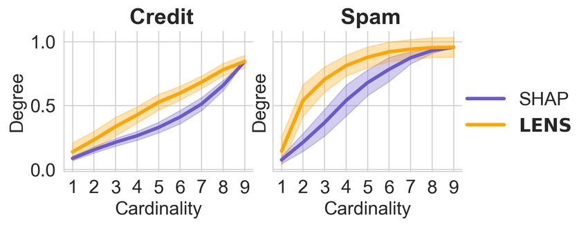
The probability that factor set C = {c1 , . . . , ck } is neces-   the most τ -minimal factors of any method with fixed type I
sary for y is given by:                                            error α.
                         k
       P N (C, y) := P (
                        X
                           ci (z) ≥ 1 | f (z) = y).                Multiple testing adjustments can easily be accommodated,
                          i=1
                                                                   in which case modified optimality criteria apply [Storey,
                                                                   2007].
Remark 1. These probabilities can be likened to the “pre-
cision” (positive predictive value) and “recall” (true posi-       Remark 2. We take it that the main quantity of interest
tive rate) of a (hypothetical) classifier that predicts whether    in most applications is sufficiency, be it for the original or
f (z) = y based on whether c(z) = 1. By examining the              alternative outcome, and therefore define τ -minimality w.r.t.
confusion matrix of this classifier, one can define other          sufficient (rather than necessary) factors. However, necessity
related quantities, e.g. the true negative rate P (c(z) =          serves an important role in tuning τ , as there is an inherent
0|f (z) 6= y) and the negative predictive value P (f (z) 6=        trade-off between the parameters. More factors are excluded
y|c(z) = 0), which are contrapositive transformations of           at higher values of τ , thereby inducing lower cumulative
our proposed measures. We can recover these values exactly         P N ; more factors are included at lower values of τ , thereby
via P S(1 − c, 1 − y) and P N (1 − c, 1 − y), respectively.        inducing higher cumulative P N . See Appendix B.
When necessity and sufficiency are defined as probabilistic
inversions (rather than conversions), such transformations         Algorithm 1 LENS
are impossible.                                                     1: Input: B = hf, D, C, i, τ
                                                                    2: Output: Factor set C, (∀c ∈ C) P S(c, y), P N (C, y)
3.2   MINIMAL SUFFICIENT FACTORS
                                                                    3: Sample D̂ = {zi }n
                                                                                        i=1 ∼ D
We introduce Local Explanations via Necessity and Suffi-
ciency (LENS), a procedure for computing explanatory fac-                          Pn (c, y)
                                                                    4: function probSuff
tors with respect to a given basis B and threshold parame-          5:   n(c&y)P = i=1 1[c(zi ) = 1 ∧ f (zi ) = y]
                                                                                  n
ter τ (see Alg. 1). First, we calculate a factor’s probability      6:   n(c) = i=1 c(zi )
of sufficiency (see probSuff) by drawing n samples from             7:   return n(c&y) / n(c)
D and taking the maximum likelihood estimate PˆS(c, y).
Next, we sort the space of factors w.r.t.  in search of those      8: function probNec(C, y, upward_closure_flag)
that are τ -minimal.                                                9:   if upward_closure_flag then
                                                                   10:      C = {c | c ∈ C ∧ ∃ c0 ∈ C : c0  c}
Definition 4 (τ -minimality). We say that c is τ -minimal iff      11:   end if
(i) P S(c, y) ≥ τ and (ii) there exists no factor c0 such that
                                                                                   Pn       Pk
                                                                   12:   n(C&y) = i=1 1[ j=1 cj (zi ) ≥ 1 ∧ f (zi ) = y]
P S(c0 , y) ≥ τ and c0 ≺ c.                                        13:
                                                                                Pn
                                                                         n(y) = i=1 1[f (zi ) = y]
                                                                   14:   return n(C&y) / n(y)
Since a factor is necessary to the extent that it covers all
possible pathways towards a given outcome, our next step is        15: function minimalSuffFactors(y, τ , sample_flag, α)
to span the τ -minimal factors and compute their cumulative        16:   sorted_factors = topological_sort(C, )
P N (see probNec). As a minimal factor c stands for all c0         17:   cands = []
such that c  c0 , in reporting probability of necessity, we       18:   for c in sorted_factors do
expand C to its upward closure.                                    19:     if ∃(c0 , _) ∈ cands : c0  c then
Thms. 1 and 2 state that this procedure is optimal in a sense      20:        continue
that depends on whether we assume access to oracle or              21:     end if
sample estimates of P S (see Appendix A for all proofs).           22:     ps = probSuff(c, y)
                                                                   23:     if sample_flag then
Theorem 1. With oracle estimates P S(c, y) for all c ∈ C,          24:        p = binom.test(n(c&y), n(c), τ , alt = >)
Alg. 1 is sound and complete. That is, for any C returned          25:        if p ≤ α then
by Alg. 1 and all c ∈ C, c is τ -minimal iff c ∈ C.                26:           cands.append(c, ps)
                                                                   27:        end if
Population proportions may be obtained if data fully saturate      28:     else if ps ≥ τ then
the space D, a plausible prospect for categorical variables        29:        cands.append(c, ps)
of low to moderate dimensionality. Otherwise, proportions          30:     end if
will need to be estimated.                                         31:   end for
                                                                   32:   cum_pn = probNec({c | (c, _) ∈ cands}, y, T RUE )
Theorem 2. With sample estimates PˆS(c, y) for all c ∈ C,          33:   return cands, cum_pn
Alg. 1 is uniformly most powerful. That is, Alg. 1 identifies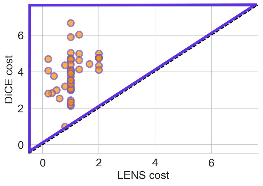
4       ENCODING EXISTING MEASURES                                     “since there is no standard procedure for converting Shapley
                                                                       values into a statement about a model’s behavior, developers
Explanatory measures can be shown to play a central role in            rely on their own mental model of what the values represent”
many seemingly unrelated XAI tools, albeit under different             (p. 8). By contrast, necessary and sufficient factors are more
assumptions about the basis tuple B. In this section, we               transparent and informative, offering a direct path to what
relate our framework to a number of existing methods.                  Shapley values indirectly summarize.

Feature attributions. Several popular feature attribution              Rule lists. Rule lists are sequences of if-then statements
algorithms are based on Shapley values [Shapley, 1953],                that describe a hyperrectangle in feature space, creating par-
which decompose the predictions of any target function as a            titions that can be visualized as decision or regression trees.
sum of weights over d input features:                                  Rule lists have long been popular in XAI. While early work
                                                                       in this area tended to focus on global methods [Friedman
                                       d
                                       X                               and Popescu, 2008; Letham et al., 2015], more recent efforts
                      f (xi ) = φ0 +         φj ,               (1)
                                                                       have prioritized local explanation tasks [Lakkaraju et al.,
                                       j=1
                                                                       2019; Sokol and Flach, 2020].
where φ0 represents a baseline expectation and φj the                  We focus in particular on the Anchors algorithm [Ribeiro
weight assigned to Xj at point xi . Let v : 2d 7→ R be a               et al., 2018a], which learns a set of Boolean conditions A
value function such that v(S) is the payoff associated with            (the eponymous “anchors”) such that A(xi ) = 1 and
feature subset S ⊆ [d] and v({∅}) = 0. Define the comple-
ment R = [d]\S such that we may rewrite any xi as a pair                                PD(x|A) (f (xi ) = f (x)) ≥ τ.                 (4)
of subvectors, (xSi , xR
                       i ). Payoffs are given by:
                                                                       The lhs of Eq. 4 is termed the precision, prec(A), and proba-
                     v(S) = E[f (xSi , X R )],                  (2)    bility is taken over a synthetic distribution in which the con-
                                                                       ditions in A hold while other features are perturbed. Once τ
although this introduces some ambiguity regarding the ref-             is fixed, the goal is to maximize coverage, formally defined
erence distribution for X R (more on this below). The Shap-            as E[A(x) = 1], i.e. the proportion of datapoints to which
ley value φj is then j’s average marginal contribution to all          the anchor applies.
subsets that exclude it:
                                                                       The formal similarities between Eq. 4 and Def. 2 are imme-
           X         |S|!(d − |S| − 1)!                                diately apparent, and the authors themselves acknowledge
 φj =                                   v(S ∪ {j}) − v(S). (3)
                             d!                                        that Anchors are intended to provide “sufficient conditions”
         S⊆[d]\{j}
                                                                       for model predictions.
It can be shown that this is the unique solution to the attri-         Proposition 2. Let cA (z) = 1 iff A(x) = 1. Then
bution problem that satisfies certain desirable properties, in-        prec(A) = P S(cA , y).
cluding efficiency, linearity, sensitivity, and symmetry.
Reformulating this in our framework, we find that the value            While Anchors outputs just a single explanation, our method
function v is a sufficiency measure. To see this, let each             generates a ranked list of candidates, thereby offering a
z ∼ D be a sample in which a random subset of variables                more comprehensive view of model behavior. Moreover, our
S are held at their original values, while remaining features          necessity measure adds a mode of explanatory information
R are drawn from a fixed distribution D(·|S).1                         entirely lacking in Anchors.

Proposition 1. Let cS (z) = 1 iff x ⊆ z was constructed                Counterfactuals. Counterfactual explanations identify
by holding xS fixed and sampling X R according to D(·|S).              one or several nearest neighbors with different outcomes, e.g.
Then v(S) = P S(cS , y).                                               all datapoints x within an -ball of xi such that labels f (x)
                                                                       and f (xi ) differ (for classification) or f (x) > f (xi ) + δ
Thus, the Shapley value φj measures Xj ’s average marginal             (for regression).2 The optimization problem is:
increase to the sufficiency of a random feature subset. The
advantage of our method is that, by focusing on particular                              x∗ = argmin cost(xi , x),                      (5)
                                                                                               x∈CF(xi )
subsets instead of weighting them all equally, we disregard
irrelevant permutations and home in on just those that meet            where CF(xi ) denotes a counterfactual space such that
a τ -minimality criterion. Kumar et al. [2020] observe that,           f (xi ) 6= f (x) and cost is a user-supplied cost function, typ-
    1
                                                                       ically equated with some distance measure. [Wachter et al.,
     The diversity of Shapley value algorithms is largely due to
                                                                           2
variation in how this distribution is defined. Popular choices in-           Confusingly, the term “counterfactual” in XAI refers to any
clude the marginal P (X R ) [Lundberg and Lee, 2017]; conditional      point with an alternative outcome, which is distinct from the causal
P (X R |xS ) [Aas et al., 2019]; and interventional P (X R |do(xS ))   sense of the term (see Sect. 2). We use the word in both senses
[Heskes et al., 2020] distributions.                                   here, but strive to make our intended meaning explicit in each case.
2018] recommend using generative adversarial networks
to solve Eq. 5, while others have proposed alternatives de-
signed to ensure that counterfactuals are coherent and ac-
tionable [Ustun et al., 2019; Karimi et al., 2020a; Wexler
et al., 2020]. As with Shapley values, the variation in these
proposals is reducible to the choice of context D.
For counterfactuals, we rewrite the objective as a search for
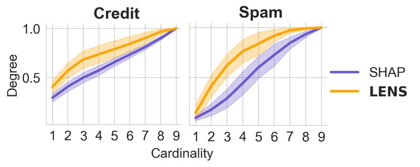
minimal perturbations sufficient to flip an outcome. Figure 2: Comparison of top k features ranked by SHAP
against the best performing LENS subset of size k in
Proposition 3. Let cost be a function representing , and
terms of P S(c, y). German results are over 50 inputs;
let c be some factor spanning reference values. Then the
SpamAssassins results are over 25 inputs.
counterfactual recourse objective is:
c∗ = argmin cost(c) s.t. P S(c, 1 − y) ≥ τ, (6) 5 EXPERIMENTS
c∈C
In this section, we demonstrate the use of LENS on a va-
where τ denotes a decision threshold. Counterfactual out-
riety of tasks and compare results with popular XAI tools,
puts will then be any z ∼ D such that c∗ (z) = 1.
using the basis configurations detailed in Table 1. A com-
prehensive discussion of experimental design, including
Probabilities of causation. Our framework can describe datasets and pre-processing pipelines, is left to Appendix
Pearl [2000]’s aforementioned probabilities of causation, C. Code for reproducing all results is available at https:
however in this case D must be constructed with care. //github.com/limorigu/LENS.
Proposition 4. Consider the bivariate Boolean setting, as Contexts. We consider a range of contexts D in our exper-
in Sect. 2. We have two counterfactual distributions: an in- iments. For the input-to-reference (I2R) setting, we replace
put space I, in which we observe x, y but intervene to set input values with reference values for feature subsets S; for
X = x0 ; and a reference space R, in which we observe x0 , y 0 the reference-to-input (R2I) setting, we replace reference
but intervene to set X = x. Let D denote a uniform mixture values with input values. We use R2I for examining suffi-
over both spaces, and let auxiliary variable W tag each sam- ciency/necessity of the original model prediction, and I2R
ple with a label indicating whether it comes from the origi- for examining sufficiency/necessity of a contrastive model
nal (W = 1) or contrastive (W = 0) counterfactual space. prediction. We sample from the empirical data in all exper-
Define c(z) = w. Then we have suf(x, y) = P S(c, y) and iments, except in Sect. 5.3, where we assume access to a
nec(x, y) = P S(1 − c, y 0 ). structural causal model (SCM).
Partial Orderings. We consider two types of partial or-
In other words, we regard Pearl’s notion of necessity as suf-
derings in our experiments. The first, subset , evaluates
ficiency of the negated factor for the alternative outcome.
subset relationships. For instance, if c(z) = 1[x[gender =
By contrast, Pearl [2000] has no analogue for our proba-
“female”]] and c0 (z) = 1[x[gender = “female” ∧
bility of necessity. This is true of any measure that defines
age ≥ 40]], then we say that c subset c0 . The second,
sufficiency and necessity via inverse, rather than converse
c cost c0 := c subset c0 ∧ cost(c) ≤ cost(c0 ), adds the
probabilities. While conditioning on the same variable(s)
additional constraint that c has cost no greater than c0 . The
for both measures may have some intuitive appeal, it comes
cost function could be arbitrary. Here, we consider distance
at a cost to expressive power. Whereas our framework can
measures over either the entire state space or just the inter-
recover all four explanatory measures, corresponding to the
vention targets corresponding to c.
classical definitions and their contrapositive forms, defini-
tions that merely negate instead of transpose the antecedent
and consequent are limited to just two. 5.1 FEATURE ATTRIBUTIONS
Remark 3. We have assumed that factors and outcomes Feature attributions are often used to identify the top-k most
are Boolean throughout. Our results can be extended to important features for a given model outcome [Barocas et al.,
continuous versions of either or both variables, so long as 2020]. However, we argue that these feature sets may not
c(Z) Y | Z. This conditional independence holds when- be explanatory with respect to a given prediction. To show
|=
ever W Y | X, which is true by construction since this, we compute R2I and I2R sufficiency – i.e., P S(c, y)
|=
f (z) := f (x). However, we defend the Boolean assump- and P S(1 − c, 1 − y), respectively – for the top-k most in-
tion on the grounds that it is well motivated by contrastivist fluential features (k ∈ [1, 9]) as identified by SHAP [Lund-
epistemologies [Kahneman and Miller, 1986; Lipton, 1990; berg and Lee, 2017] and LENS. Fig. 2 shows results from
Blaauw, 2013] and not especially restrictive, given that parti- the R2I setting for German credit [Dua and Graff, 2017]
tions of arbitrary complexity may be defined over Z and Y . and SpamAssassin datasets [SpamAssassin, 2006]. OurTable 1: Overview of experimental settings by basis configuration.
Experiment Datasets f D C
Attribution comparison German, SpamAssassins Extra-Trees R2I, I2R Intervention targets -
Anchors comparison: Brittle predictions IMDB LSTM R2I, I2R Intervention targets subset
Anchors comparison: PS and Prec German Extra-Trees R2I Intervention targets subset
Counterfactuals: Adverserial SpamAssassins MLP R2I Intervention targets subset
Counterfactuals: Recourse, DiCE comparison Adult MLP I2R Full interventions cost
Counterfactuals: Recourse, causal vs. non-causal German Extra-Trees I2Rcausal Full interventions cost
method attains higher P S for all cardinalities. We repeat
the experiment over 50 inputs, plotting means and 95% con-
fidence intervals for all k. Results indicate that our rank-
ing procedure delivers more informative explanations than
SHAP at any fixed degree of sparsity. Results from the I2R
setting are in Appendix C.
5.2 RULE LISTS
Figure 3: We compare P S(c, y) against precision scores at-
Sentiment sensitivity analysis. Next, we use LENS to tained by the output of LENS and Anchors for examples
study model weaknesses by considering minimal factors from German. We repeat the experiment for 100 inputs,
with high R2I and I2R sufficiency in text models. Our and each time consider the single example generated by An-
goal is to answer questions of the form, “What are words chors against the mean P S(c, y) among LENS’s candidates.
with/without which our model would output the origi- Dotted line indicates τ = 0.9.
nal/opposite prediction for an input sentence?” For this ex-
periment, we train an LSTM network on the IMDB dataset errors, or test for model reliance on sensitive attributes (e.g.,
for sentiment analysis [Maas et al., 2011]. If the model mis- gender pronouns).
labels a sample, we investigate further; if it does not, we
Anchors comparison. Anchors also includes a tabular
inspect the most explanatory factors to learn more about
variant, against which we compare LENS’s performance
model behavior. For the purpose of this example, we only
in terms of R2I sufficiency. We present the results of this
inspect sentences of length 10 or shorter. We provide two
comparison in Fig. 3, and include additional comparisons
examples below and compare with Anchors (see Table 2).
in Appendix C. We sample 100 inputs from the German
Consider our first example: READ BOOK FORGET MOVIE is dataset, and query both methods with τ = 0.9 using the
a sentence we would expect to receive a negative prediction, classifier from Sect. 5.1. Anchors satisfies a PAC bound
but our model classifies it as positive. Since we are inves- controlled by parameter δ. At the default value δ = 0.1,
tigating a positive prediction, our reference space is condi- Anchors fails to meet the τ threshold on 14% of samples;
tioned on a negative label. For this model, the classic UNK LENS meets it on 100% of samples. This result accords
token receives a positive prediction. Thus we opt for an al- with Thm. 1, and vividly demonstrates the benefits of our
ternative, PLATE. Performing interventions on all possible optimality guarantee. Note that we also go beyond Anchors
combinations of words with our token, we find the conjunc- in providing multiple explanations instead of just a single
tion of READ , FORGET, and MOVIE is a sufficient factor for output, as well as a cumulative probability measure with no
a positive prediction (R2I). We also find that changing any analogue in their algorithm.
of READ, FORGET, or MOVIE to PLATE would result in a
negative prediction (I2R). Anchors, on the other hand, per-
turbs the data stochastically (see Appendix C), suggesting 5.3 COUNTERFACTUALS
the conjunction READ AND BOOK. Next, we investigate
the sentence: YOU BETTER CHOOSE PAUL VERHOEVEN Adversarial examples: spam emails. R2I sufficiency an-
EVEN WATCHED . Since the label here is negative, we use swers questions of the form, “What would be sufficient
the UNK token. We find that this prediction is brittle – a for the model to predict y?”. This is particularly valuable
change of almost any word would be sufficient to flip the in cases with unfavorable outcomes y 0 . Inspired by adver-
outcome. Anchors, on the other hand, reports a conjunction sarial interpretability approaches [Ribeiro et al., 2018b;
including most words in the sentence. Taking the R2I view, Lakkaraju and Bastani, 2020], we train an MLP classifier
we still find a more concise explanation: CHOOSE or EVEN on the SpamAssassins dataset and search for minimal
would be enough to attain a negative prediction. These brief factors sufficient to relabel a sample of spam emails as non-
examples illustrate how LENS may be used to find brittle spam. Our examples follow some patterns common to spam
predictions across samples, search for similarities between emails: received from unusual email addresses, includes sus-Table 2: Example prediction given by an LSTM model trained on the IMDB dataset. We compare τ -minimal factors identified
by LENS (as individual words), based on P S(c, y) and P S(1 − c, 1 − y), and compare to output by Anchors.
Inputs Anchors LENS
Text Original model prediction Suggested anchors Precision Sufficient R2I factors Sufficient I2R factors
’read book forget movie’ wrongly predicted positive [read, movie] 0.94 [read, forget, movie] read, forget, movie
’you better choose paul verhoeven even watched’ correctly predicted negative [choose, better, even, you, paul, verhoeven] 0.95 choose, even better, choose, paul, even
Table 3: (Top) A selection of emails from SpamAssassins, correctly identified as spam by an MLP. The goal is to find
minimal perturbations that result in non-spam predictions. (Bottom) Minimal subsets of feature-value assignments that
achieve non-spam predictions with respect to the emails above.
From To Subject First Sentence Last Sentence
resumevalet info resumevalet com yyyy cv spamassassin taint org adv put resume back work dear candidate professionals online network inc
jacqui devito goodroughy ananzi co za picone linux midrange com enlargement breakthrough zibdrzpay recent survey conducted increase size enter detailsto come open
rose xu email com yyyyac idt net adv harvest lots target email address quickly want advertisement persons 18yrs old
Gaming options Feature subsets for value changes
From To
1
crispin cown crispin wirex com example com mailing... list secprog securityfocus... moderator
From First Sentence
2
crispin cowan crispin wirex com scott mackenzie wrote
From First Sentence
3
tim one comcast net tim peters tim
picious keywords such as ENLARGEMENT or ADVERTISE - Figure 4: A comparison of mean cost of outputs by LENS
MENT in the subject line, etc. We identify minimal changes and DiCE for 50 inputs sampled from the Adult dataset.
that will flip labels to non-spam with high probability. Op-
tions include altering the incoming email address to more
common domains, and changing the subject or first sen- factor c from a method M is minimally valid iff for all c0 pro-
tences (see Table 3). These results can improve understand- posed by M 0 , ¬(c0 ≺cost c) (i.e., M 0 does not report a fac-
ing of both a model’s behavior and a dataset’s properties. tor preferable to c). We report results based on 50 randomly
sampled inputs from the Adult dataset, where references
Diverse counterfactuals. Our explanatory measures can
are fixed by conditioning on the opposite prediction. The
also be used to secure algorithmic recourse. For this experi-
cost comparison results are shown in Fig. 4, where we find
ment, we benchmark against DiCE [Mothilal et al., 2020b],
that LENS identifies lower cost factors for the vast majority
which aims to provide diverse recourse options for any
of inputs. Furthermore, DiCE finds no minimally valid can-
underlying prediction model. We illustrate the differences
didates that LENS did not already account for. Thus LENS
between our respective approaches on the Adult dataset
emphasizes minimality and diversity of intervention targets,
[Kochavi and Becker, 1996], using an MLP and following
while still identifying low cost intervention values.
the procedure from the original DiCE paper.
According to DiCE, a diverse set of counterfactuals is
Causal vs. non-causal recourse. When a user relies on
one that differs in values assigned to features, and can
XAI methods to plan interventions on real-world systems,
thus produce a counterfactual set that includes different
causal relationships between predictors cannot be ignored.
interventions on the same variables (e.g., CF1: age =
In the following example, we consider the DAG in Fig. 5,
91, occupation = “retired”; CF2: age = 44, occupation =
intended to represent dependencies in the German credit
“teacher”). Instead, we look at diversity of counterfactuals
dataset. For illustrative purposes, we assume access to the
in terms of intervention targets, i.e. features changed (in
structural equations of this data generating process. (There
this case, from input to reference values) and their effects.
are various ways to extend our approach using only partial
We present minimal cost interventions that would lead to re-
causal knowledge as input [Karimi et al., 2020b; Heskes
course for each feature set but we summarize the set of paths
et al., 2020].) We construct D by sampling from the SCM
to recourse via subsets of features changed. Thus, DiCE pro-
under a series of different possible interventions. Table 4
vides answers of the form “Because you are not 91 and re-
describes an example of how using our framework with
tired” or “Because you are not 44 and a teacher”; we answer
augmented causal knowledge can lead to different recourse
“Because of your age and occupation”, and present the low-
options. Computing explanations under the assumption of
est cost intervention on these features sufficient to flip the
feature independence results in factors that span a large
prediction.
part of the DAG depicted in Fig. 5. However, encoding
With this intuition in mind, we compare outputs given by structural relationships in D, we find that LENS assigns
DiCE and LENS for various inputs. For simplicity, we let high explanatory value to nodes that appear early in the
all features vary independently. We consider two metrics for topological ordering. This is because intervening on a single
comparison: (a) the mean cost of proposed factors, and (b) root factor may result in various downstream changes once
the number of minimally valid candidates proposed, where a effects are fully propagated.Table 4: Recourse example comparing causal and non-causal (i.e., feature independent) D. We sample a single input
example with a negative prediction, and 100 references with the opposite outcome. For I2Rcausal we propagate the effects
of interventions through a user-provided SCM.
input I2R I2Rcausal
Age Sex Job Housing Savings Checking Credit Duration Purpose τ -minimal factors (τ = 0) Cost τ -minimal factors (τ = 0) Cost
Job: Highly skilled 1 Age: 24 0.07
Checking: NA 1 Sex: Female 1
23 Male Skilled Free Little Little 1845 45 Radio/TV Duration: 30 1.25 Job: Highly skilled 1
Age: 65, Housing: Own 4.23 Housing: Rent 1
Age: 34, Savings: N/A 1.84 Savings: N/A 1
Checking where explanations are more meaningful to end users. For
Sex Duration
instance, in our SpamAssassins experiments, we started
Job Savings Housing P urpose with a pure text example, which can be represented via
Age
Credit
high-dimensional vectors (e.g., word embeddings). How-
ever, we represent the data with just a few intelligible com-
ponents: From and To email addresses, Subject, etc. In
other words, we create a more abstract object and consider
Figure 5: Example DAG for German dataset. each segment as a potential intervention target, i.e. a candi-
date factor. This effectively compresses a high-dimensional
dataset into a 10-dimensional abstraction. Similar strategies
6 DISCUSSION could be used in many cases, either through domain knowl-
edge or data-driven clustering and dimensionality reduction
Our results, both theoretical and empirical, rely on access to techniques [Chalupka et al., 2017; Beckers et al., 2019; Lo-
the relevant context D and the complete enumeration of all catello et al., 2019]. In general, if data cannot be represented
feature subsets. Neither may be feasible in practice. When by a reasonably low-dimensional, intelligible abstraction,
elements of Z are estimated, as is the case with the genera- then post-hoc XAI methods are unlikely to be of much help.
tive methods sometimes used in XAI, modeling errors could
lead to suboptimal explanations. For high-dimensional set-
tings such as image classification, LENS cannot be naïvely 7 CONCLUSION
applied without substantial data pre-processing. The first is-
sue is extremely general. No method is immune to model We have presented a unified framework for XAI that fore-
misspecification, and attempts to recreate a data generat- grounds necessity and sufficiency, which we argue are the
ing process must always be handled with care. Empirical fundamental building blocks of all successful explanations.
sampling, which we rely on above, is a reasonable choice We defined simple measures of both, and showed how they
when data are fairly abundant and representative. However, undergird various XAI methods. Our formulation, which re-
generative models may be necessary to correct for known lies on converse rather than inverse probabilities, is uniquely
biases or sample from low-density regions of the feature flexible and expressive. It covers all four basic explanatory
space. This comes with a host of challenges that no XAI al- measures – i.e., the classical definitions and their contra-
gorithm alone can easily resolve. The second issue – that positive transformations – and unambiguously accommo-
a complete enumeration of all variable subsets is often im- dates logical, probabilistic, and/or causal interpretations, de-
practical – we consider to be a feature, not a bug. Complex pending on how one constructs the basis tuple B. We illus-
explanations that cite many contributing factors pose cog- trated illuminating connections between our measures and
nitive as well as computational challenges. In an influen- existing proposals in XAI, as well as Pearl [2000]’s proba-
tial review of XAI, Miller [2019] finds near unanimous con- bilities of causation. We introduced a sound and complete
sensus among philosophers and social scientists that, “all algorithm for identifying minimally sufficient factors, and
things being equal, simpler explanations – those that cite demonstrated our method on a range of tasks and datasets.
fewer causes... are better explanations” (p. 25). Even if we Our approach prioritizes completeness over efficiency, suit-
could list all τ -minimal factors for some very large value of able for settings of moderate dimensionality. Future research
d, it is not clear that such explanations would be helpful to will explore more scalable approximations, model-specific
humans, who famously struggle to hold more than seven ob- variants optimized for, e.g., convolutional neural networks,
jects in short-term memory at any given time [Miller, 1955]. and developing a graphical user interface.
That is why many popular XAI tools include some sparsity
constraint to encourage simpler outputs.
Acknowledgements
Rather than throw out some or most of our low-level fea-
tures, we prefer to consider a higher level of abstraction, DSW was supported by ONR grant N62909-19-1-2096.References Sachin Grover, Chiara Pulice, Gerardo I. Simari, and V. S.
Subrahmanian. Beef: Balanced english explanations of
Kjersti Aas, Martin Jullum, and Anders Løland. Explain- forecasts. IEEE Trans. Comput. Soc. Syst., 6(2):350–364,
ing individual predictions when features are dependent: 2019.
More accurate approximations to Shapley values. arXiv
preprint, 1903.10464v2, 2019. Joseph Y Halpern. Actual Causality. The MIT Press, Cam-
bridge, MA, 2016.
Solon Barocas, Andrew D Selbst, and Manish Raghavan.
The Hidden Assumptions behind Counterfactual Explana- Joseph Y Halpern and Judea Pearl. Causes and explanations:
tions and Principal Reasons. In FAT*, pages 80–89, 2020. A structural-model approach. Part I: Causes. Br. J. Philos.
Sci., 56(4):843–887, 2005a.
Sander Beckers, Frederick Eberhardt, and Joseph Y Halpern.
Joseph Y Halpern and Judea Pearl. Causes and explanations:
Approximate causal abstraction. In UAI, pages 210–219,
A structural-model approach. Part II: Explanations. Br. J.
2019.
Philos. Sci., 56(4):889–911, 2005b.
Umang Bhatt, Alice Xiang, Shubham Sharma, Adrian Tom Heskes, Evi Sijben, Ioan Gabriel Bucur, and Tom
Weller, Ankur Taly, Yunhan Jia, Joydeep Ghosh, Ruchir Claassen. Causal Shapley values: Exploiting causal
Puri, José M F Moura, and Peter Eckersley. Explainable knowledge to explain individual predictions of complex
machine learning in deployment. In FAT*, pages 648– models. In NeurIPS, 2020.
657, 2020.
Alexey Ignatiev, Nina Narodytska, and Joao Marques-Silva.
Steven Bird, Ewan Klein, and Edward Loper. Natural lan- Abduction-based explanations for machine learning mod-
guage processing with Python: Analyzing text with the els. In AAAI, pages 1511–1519, 2019.
natural language toolkit. O’Reilly, 2009.
Guido W Imbens and Donald B Rubin. Causal Inference
Martijn Blaauw, editor. Contrastivism in Philosophy. Rout- for Statistics, Social, and Biomedical Sciences: An Intro-
ledge, New York, 2013. duction. Cambridge University Press, Cambridge, 2015.
Krzysztof Chalupka, Frederick Eberhardt, and Pietro Perona. Daniel Kahneman and Dale T. Miller. Norm theory: Com-
Causal feature learning: an overview. Behaviormetrika, paring reality to its alternatives. Psychol. Rev., 93(2):136–
44(1):137–164, 2017. 153, 1986.
Amit Dhurandhar, Pin-Yu Chen, Ronny Luss, Chun-Chen Amir-Hossein Karimi, Gilles Barthe, Bernhard Schölkopf,
Tu, Paishun Ting, Karthikeyan Shanmugam, and Payel and Isabel Valera. A survey of algorithmic recourse:
Das. Explanations based on the missing: Towards con- Definitions, formulations, solutions, and prospects. arXiv
trastive explanations with pertinent negatives. In NeurIPS, preprint, 2010.04050, 2020a.
pages 592–603, 2018.
Amir-Hossein Karimi, Julius von Kügelgen, Bernhard
Schölkopf, and Isabel Valera. Algorithmic recourse under
Dheeru Dua and Casey Graff. UCI machine learning
imperfect causal knowledge: A probabilistic approach. In
repository, 2017. URL http://archive.ics.uci.
NeurIPS, 2020b.
edu/ml.
Diederik P. Kingma and Jimmy Ba. Adam: A method for
C. Fernández-Loría, F. Provost, and X. Han. Explaining
stochastic optimization. In The 3rd International Confer-
data-driven decisions made by AI systems: The counter-
ence for Learning Representations, 2015.
factual approach. arXiv preprint, 2001.07417, 2020.
Ronny Kochavi and Barry Becker. Adult income dataset,
Jerome H Friedman and Bogdan E Popescu. Predictive 1996. URL https://archive.ics.uci.edu/
learning via rule ensembles. Ann. Appl. Stat., 2(3):916– ml/datasets/adult.
954, 2008.
Indra Kumar, Suresh Venkatasubramanian, Carlos Scheideg-
Sainyam Galhotra, Romila Pradhan, and Babak Salimi. Ex- ger, and Sorelle Friedler. Problems with Shapley-value-
plaining black-box algorithms using probabilistic con- based explanations as feature importance measures. In
trastive counterfactuals. In SIGMOD, 2021. ICML, pages 5491–5500, 2020.
Pierre Geurts, Damien Ernst, and Louis Wehenkel. Ex- Himabindu Lakkaraju and Osbert Bastani. “How do I fool
tremely randomized trees. Mach. Learn., 63(1):3–42, you?”: Manipulating user trust via misleading black box
2006. explanations. In AIES, pages 79–85, 2020.Himabindu Lakkaraju, Ece Kamar, Rich Caruana, and Jure Ramaravind K. Mothilal, Amit Sharma, and Chenhao Tan.
Leskovec. Faithful and customizable explanations of Explaining machine learning classifiers through diverse
black box models. In AIES, pages 131–138, 2019. counterfactual explanations. In FAT*, pages 607–617,
2020b.
E.L. Lehmann and Joseph P. Romano. Testing Statistical
Hypotheses. Springer, New York, Third edition, 2005. Nina Narodytska, Aditya Shrotri, Kuldeep S Meel, Alexey
Ignatiev, and Joao Marques-Silva. Assessing heuristic
Benjamin Letham, Cynthia Rudin, Tyler H McCormick, and machine learning explanations with model counting. In
David Madigan. Interpretable classifiers using rules and SAT, pages 267–278, 2019.
Bayesian analysis: Building a better stroke prediction
Judea Pearl. Causality: Models, Reasoning, and Inference.
model. Ann. Appl. Stat., 9(3):1350–1371, 2015.
Cambridge University Press, New York, 2000.
David Lewis. Causation. J. Philos., 70:556–567, 1973. Jeffrey Pennington, Richard Socher, and Christopher D Man-
ning. GloVe: Global vectors for word representation. In
Peter Lipton. Contrastive explanation. Royal Inst. Philos.
EMNLP, pages 1532–1543, 2014.
Suppl., 27:247–266, 1990.
Yanou Ramon, David Martens, Foster Provost, and
Zachary Lipton. The mythos of model interpretability. Com- Theodoros Evgeniou. A comparison of instance-level
mun. ACM, 61(10):36–43, 2018. counterfactual explanation algorithms for behavioral and
textual data: SEDC, LIME-C and SHAP-C. Adv. Data
Francesco Locatello, Stefan Bauer, Mario Lucic, Gunnar
Anal. Classif., 2020.
Raetsch, Sylvain Gelly, Bernhard Schölkopf, and Olivier
Bachem. Challenging common assumptions in the un- Marco Túlio Ribeiro, Sameer Singh, and Carlos Guestrin.
supervised learning of disentangled representations. In Anchors: High-precision model-agnostic explanations. In
ICML, pages 4114–4124, 2019. AAAI, pages 1527–1535, 2018a.
Scott M Lundberg and Su-In Lee. A unified approach to Marco Túlio Ribeiro, Sameer Singh, and Carlos Guestrin.
interpreting model predictions. In NeurIPS, pages 4765– Semantically equivalent adversarial rules for debugging
4774. 2017. NLP models. In ACL, pages 856–865, 2018b.
Andrew L. Maas, Raymond E. Daly, Peter T. Pham, Dan Cynthia Rudin. Stop explaining black box machine learning
Huang, Andrew Y. Ng, and Christopher Potts. Learning models for high stakes decisions and use interpretable
word vectors for sentiment analysis. In ACL, pages 142– models instead. Nat. Mach. Intell., 1(5):206–215, 2019.
150, 2011. Lloyd Shapley. A value for n-person games. In Contribu-
tions to the Theory of Games, chapter 17, pages 307–317.
J.L. Mackie. Causes and conditions. Am. Philos. Q., 2(4):
Princeton University Press, Princeton, 1953.
245–264, 1965.
Kacper Sokol and Peter Flach. LIMEtree: Interactively
Luke Merrick and Ankur Taly. The explanation game: Ex- customisable explanations based on local surrogate multi-
plaining machine learning models using shapley values. output regression trees. arXiv preprint, 2005.01427, 2020.
In CD-MAKE, pages 17–38. Springer, 2020.
Apache SpamAssassin, 2006. URL https:
George A. Miller. The magical number seven, plus or minus //spamassassin.apache.org/old/
two: Some limits on our capacity for processing informa- publiccorpus/. Accessed 2021.
tion. Psychol. Rev., 101(2):343–352, 1955.
John D Storey. The optimal discovery procedure: A new
Tim Miller. Explanation in artificial intelligence: Insights approach to simultaneous significance testing. J. Royal
from the social sciences. Artif. Intell., 267:1–38, 2019. Stat. Soc. Ser. B Methodol., 69(3):347–368, 2007.
Mukund Sundararajan and Amir Najmi. The many Shapley
Christoph Molnar. Interpretable Machine Learning: A
values for model explanation. In ACM, New York, 2019.
Guide for Making Black Box Models Interpretable.
Münich, 2021. URL https://christophm. Jin Tian and Judea Pearl. Probabilities of causation: Bounds
github.io/interpretable-ml-book/. and identification. Ann. Math. Artif. Intell., 28(1-4):287–
313, 2000.
Ramaravind K. Mothilal, Divyat Mahajan, Chenhao Tan,
and Amit Sharma. Towards unifying feature attribution Berk Ustun, Alexander Spangher, and Yang Liu. Actionable
and counterfactual explanations: Different means to the recourse in linear classification. In FAT*, pages 10–19,
same end. arXiv preprint, 2011.04917, 2020a. 2019.Tyler J VanderWeele and Thomas S Richardson. General some c ∈ C for which either the algorithm failed to properly
theory for interactions in sufficient cause models with evaluate P S(c, y), thereby violating (P3); or wrongly iden-
dichotomous exposures. Ann. Stat., 40(4):2128–2161, tified some c0 such that (i) P S(c0 , y) ≥ τ and (ii) c0 ≺ c.
2012. Once again, (i) is impossible by (P3), and (ii) is impossible
by (P2). Thus there can be no false negatives.
Tyler J VanderWeele and James M Robins. Empirical and
counterfactual conditions for sufficient cause interactions.
Biometrika, 95(1):49–61, 2008. A.1.2 Proof of Theorem 2
John von Neumann and Oskar Morgenstern. Theory of Theorem. With sample estimates PˆS(c, y) for all c ∈ C,
Games and Economic Behavior. Princeton University Alg. 1 is uniformly most powerful.
Press, Princeton, NJ, 1944.
Proof. A testing procedure is uniformly most powerful
Sandra Wachter, Brent Mittelstadt, and Chris Russell. Coun-
(UMP) if it attains the lowest type II error β of all tests with
terfactual explanations without opening the black box:
fixed type I error α. Let Θ0 , Θ1 denote a partition of the pa-
Automated decisions and the GDPR. Harvard J. Law
rameter space into null and alternative regions, respectively.
Technol., 31(2):841–887, 2018.
The goal in frequentist inference is to test the null hypoth-
David S Watson and Luciano Floridi. The explanation game: esis H0 : θ ∈ Θ0 against the alternative H1 : θ ∈ Θ1 for
a formal framework for interpretable machine learning. some parameter θ. Let ψ(X) be a testing procedure of the
Synthese, 2020. form 1[T (X) ≥ cα ], where X is a finite sample, T (X) is a
test statistic, and cα is the critical value. This latter param-
J. Wexler, M. Pushkarna, T. Bolukbasi, M. Wattenberg, eter defines a rejection region such that test statistics inte-
F. Viégas, and J. Wilson. The what-if tool: Interactive grate to α under H0 . We say that ψ(X) is UMP iff, for any
probing of machine learning models. IEEE Trans. Vis. other test ψ 0 (X) such that
Comput. Graph., 26(1):56–65, 2020.
sup Eθ [ψ 0 (X)] ≤ α,
Xin Zhang, Armando Solar-Lezama, and Rishabh Singh. In- θ∈Θ0
terpreting neural network judgments via minimal, stable, we have
and symbolic corrections. In NeurIPS, page 4879–4890,
2018. (∀θ ∈ Θ1 ) Eθ [ψ 0 (X)] ≤ Eθ [ψ(X)],
where Eθ∈Θ1 [ψ(X)] denotes the power of the test to de-
tect the true θ, 1 − βψ (θ). The UMP-optimality of Alg. 1
A PROOFS follows from the UMP-optimality of the binomial test (see
[Lehmann and Romano, 2005, Ch. 3]), which is used to de-
A.1 THEOREMS cide between H0 : P S(c, y) < τ and H1 : P S(c, y) ≥ τ
on the basis of observed proportions PˆS(c, y), estimated
A.1.1 Proof of Theorem 1 from n samples for all c ∈ C. The proof now takes the same
structure as that of Thm. 1, with (P3) replaced by (P30 ): ac-
Theorem. With oracle estimates P S(c, y) for all c ∈ C, cess to UMP estimates of P S(c, y). False positives are no
Alg. 1 is sound and complete. longer impossible but bounded at level α; false negatives
are no longer impossible but occur with frequency β. Be-
Proof. Soundness and completeness follow directly from the cause no procedure can find more τ -minimal factors for any
specification of (P1) C and (P2) in the algorithm’s input fixed α, Alg. 1 is UMP.
B, along with (P3) access to oracle estimates P S(c, y) for
all c ∈ C. Recall that the partial ordering must be complete A.2 PROPOSITIONS
and transitive, as noted in Sect. 3.
A.2.1 Proof of Proposition 1
Assume that Alg. 1 generates a false positive, i.e. outputs
some c that is not τ -minimal. Then by Def. 4, either the algo-
Proposition. Let cS (z) = 1 iff x ⊆ z was constructed by
rithm failed to properly evaluate P S(c, y), thereby violating
holding xS fixed and sampling X R according to D(·|S).
(P3); or failed to identify some c0 such that (i) P S(c0 , y) ≥
Then v(S) = P S(cS , y).
τ and (ii) c0 ≺ c. (i) is impossible by (P3), and (ii) is impos-
sible by (P2). Thus there can be no false positives.
As noted in the text, D(x|S) may be defined in a variety of
Assume that Alg. 1 generates a false negative, i.e. fails to ways (e.g., via marginal, conditional, or interventional dis-
output some c that is in fact τ -minimal. By (P1), this c can- tributions). For any given choice, let cS (z) = 1 iff x is con-
not exist outside the finite set C. Therefore there must be structed by holding xSi fixed and sampling X R accordingYou can also read