How Hurricanes Sweep Up Housing Markets: Evidence from Florida
←
→
Page content transcription
If your browser does not render page correctly, please read the page content below
How Hurricanes Sweep Up Housing Markets:
            Evidence from Florida
                           Yanjun Liao*†             Yann Panassié*‡

                                     Job Market Paper
                               (click here for latest version)

                                      January 18, 2019

          This paper examines the impacts of hurricanes on the housing market and the associ-
      ated implications for local population turnover. We directly characterize equilibrium dy-
      namics in the housing market using micro-level estimates. For this purpose, we assem-
      ble a comprehensive dataset by combining housing transactions, parcel tax assessments,
      and hurricane history in Florida during 2000-2016. Our results show that hurricanes
      cause an increase in equilibrium prices and a concurrent decrease in the probability of
      transaction for homes in affected areas, both lasting up to three years. Together, these
      dynamics imply a negative transitory shock to the housing supply as a consequence of
      the hurricane. Furthermore, we match buyer characteristics from mortgage applications
      to provide the first buyer-level evidence on population turnover. We find that incom-
      ing homeowners in this period have higher incomes, leading to an overall shift in the
      local economic profile toward higher-income groups. Our findings suggest that market
      responses to destructive natural disasters can lead to uneven and lasting demographic
      changes in affected communities, even with a full recovery in physical capital.

      JEL Classification: J10, Q54, R23, R31.
      Keywords: Hurricanes, Housing Markets, Hedonic Regression, Repeat Sales Method

   * Data  provided by Zillow through the Zillow Transaction and and Assessment Dataset (ZTRAX).
More information on accessing the data can be found at http://www.zillow.com/ztrax. The results and
opinions are those of the authors and do not reflect the position of Zillow Group. We are grateful
to Richard Carson, Julie Cullen, Josh Graff Zivin, and Mark Jacobsen for helpful conversations and
insightful advice. We thank Josh Graff Zivin for his generous help with data access, and Rebecca
Fraenkel for initial data extractions. We have also benefited from comments and suggestions by Judd
Boomhower, Gordon McCord, and seminar participants at UCSD. All errors are our own.
    † Corresponding author. Email: yal005@ucsd.edu. Website: http://econweb.ucsd.edu/~yal005/.

Department of Economics, University of California, San Diego.
    ‡ Email: PanassieY@gao.gov. U.S. Government Accountability Office.

                                                 1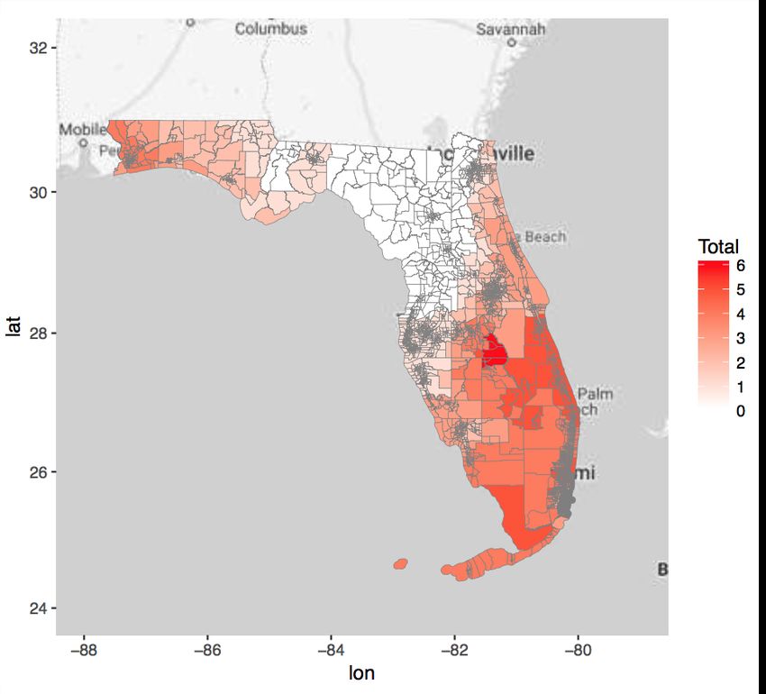
1     Introduction

About three hurricanes make landfall every year along the Gulf and east coasts of the United
States. In 2017 alone, these giant, spiraling tropical storms cost a total damage of $265
billion (USD).1 While statistics of direct property losses and fatalities are readily available,
many questions remain unanswered regarding the adjustments in the economy beyond im-
mediate impacts. Little is known about how the distribution of physical capital responds to
stochastic events like hurricanes. From a welfare perspective, the literature is only starting
to investigate how individuals cope with natural disasters and their heterogeneous ability in
doing so.2 Answering these questions is important for assessing the long-run consequences
of and adaptations to hurricanes.

    Using transaction-level housing data from Florida, this paper studies the responses to
hurricanes in housing markets for up to ten years after the hurricane strikes. The housing
market offers a unique vantage point for understanding the interaction between natural forces
and the local economy. Across localities, housing market conditions correspond closely
to changes in population and long-run economic projections (Glaeser and Gyourko, 2005).
They also determine who has access to a given location, which, in turn, affects access to
economic opportunities and a range of important local amenities (Kling et al., 2005, 2007;
Chetty et al., 2016). Therefore, studying the housing market allows us to understand how
hurricanes affect both the distribution of physical capital and the welfare of the affected
population.

    The contribution of this paper is two-fold. First, we estimate the causal impacts of hur-
ricanes on the dynamics of housing prices and transaction probability in exposed areas. To-
gether, they characterize the equilibrium adjustments in the housing market after the destruc-
tive impacts of hurricanes. While many factors in housing supply and demand can be affected
by hurricanes, this approach identifies the dominant effect and provides evidence on whether
the effect is temporary or more enduring. Second, we investigate the implications of these
    1 Recent studies in climate science observe that hurricanes have been intensifying and traveling
more slowly, possibly due to anthropogenic climate change (IPCC, 2013; Kossin, 2018). Continuation
of these trends would mean greater damages from hurricanes in the near term.
    2 This emerging literature is largely motivated by and focus on Hurricane Katrina. Earlier studies

present descriptive evidence of migratory decisions made by Katrina evacuees (Groen and Polivka,
2008; McIntosh, 2008; Paxson and Rouse, 2008; Sastry and Gregory, 2014; Fussell, 2015). More
recent studies identify causal impacts of Katrina on its victims’ employment outcome and debt level
(Gallagher and Hartley, 2017; Deryugina et al., 2018).

                                                  2
adjustments on affected neighborhoods, including potential changes in local demographics
and housing characteristics. The direction of these changes is theoretically ambiguous: the
large initial damage by hurricanes might induce further deterioration of affected communi-
ties, but it might also be neutralized in a full recovery, even lead to some type of creative
destruction, as suggested by anecdotal evidence3 and some past studies on aggregate growth
effects (Skidmore and Toya, 2002; Crespo Cuaresma et al., 2008; Pelli and Tschopp, 2017).
This paper provides the first micro-level evidence on this question.
Our analysis focuses on Florida in 2000-2016. As the most hurricane-prone state in
the U.S., Florida has experienced hurricanes with different strengths, ranging from severe
outliers – such as Hurricane Andrew and Hurricane Katrina – to milder ones. Therefore, our
results represent the impacts of an average hurricane. We assemble a detailed housing dataset
by combining transaction records and county tax assessments. The transaction data cover
95% of the universe of housing transactions. The tax assessments provide rich information
on hedonic characteristics of any given parcel in repeated observations, which we use to
infer characteristics of the transacted home with accuracy. As such, this dataset allows us
to identify and track individual parcels over time, observing most transactions and major
renovations that took place between 2000 and 2016.
We use a staggered difference-in-differences framework that exploits the randomness in
the paths and timing of several hurricanes. Treatment is defined, for individual parcels, as
being exposed to hurricane-scale wind speed. We construct a measure of exposure based
entirely on physical and geographic attributes of the hurricanes. There is an important dis-
tinction between being exposed and being damaged. An exposed house is one that lies in
the approximate area around the segment of the hurricane path with high wind speed, but
not necessarily damaged. Essentially, our strategy compares areas exposed to a hurricane to
unexposed ones before and after the hurricane.
We find that home prices increase in exposed areas in the three years following a hurri-
cane. Compared to unexposed areas, home prices in exposed areas are 5% higher on average
during this period, with a peak of 10% in the second year. This effect is identified in two
models. The first uses variation within census tract while controlling for house character-
istics, seasonality, and differential economic growth across counties. The second employs
parcel fixed effects and restricts the identifying variation to be coming from repeated sales of
the same structure. The direction and scale of the estimates are very similar across the two
3 See, for example, https://www.newyorker.com/magazine/2011/03/28/creative-destruction.
3models, providing strong evidence that the effect is mainly driven by within-home apprecia-
tion rather than a shift in the composition of transacted homes.
We also find that the transaction probability of homes in exposed areas falls by 0.6 per-
centage points, or 6% of the baseline probability. The timing of this effect is the same as the
price effect: both last around three years before returning to the baseline. Taken together,
they suggest that the housing markets at exposed areas are dominated by a negative supply
shock, but this effect is temporary. These results are consistent with the mechanism that hur-
ricanes lead to significant physical damages to and destruction of part of the housing stock,
thereby temporarily contracting available supply, and in turn, reducing sales and driving up
prices. Housing shortage of this nature has been increasingly identified by media reporting
on recent hurricane events.4 Moreover, it takes time for hurricane victims to seek financial
aid from insurance companies or federal agencies, and to eventually restore their damaged
homes to habitable or salable conditions. This explains the duration of the effect.
While the adjustment in the market equilibrium appears to be transitory, it generates last-
ing impacts on local demographics. We match a subset of our housing transactions to Home
Mortgage Disclosure Act (HMDA) records to obtain income and demographic information
of the home buyers.5 Using this subsample, we show that the average income of new buyers
increases nearly proportionally to the rise in home prices. This illustrates a greater ability of
higher-income individuals to acquire homes even in disrupted market conditions. Moreover,
both average transacted prices and buyer incomes return to the baseline level but not below
in subsequent years. The three-year increase thus leads to a stock effect of around 28% of
homes being occupied by households with higher income. In this light, hurricanes act as
a place-based policy that leads to a substantial increase in neighbors with higher income,
which could spur subsequent neighborhood improvements (Bayer et al., 2007; Card et al.,
2008; Guerrieri et al., 2013; Diamond, 2016).
Our estimation strategy combines a staggered difference-in-differences framework and
the repeat sales model. The former is common among studies that use variation from several
hurricanes, but is often applied to aggregate data. On the other hand, the latter method is
4 See, for example, the Wall Street Journal’s coverage of the impact of Hurricane Irma in Florida
Keys (https://www.wsj.com/articles/hurricane-irma-destroyed-25-of-homes-in-florida-keys) or that
of Hurricane Florence in North Carolina (https://www.wsj.com/articles/hurricane-florence-creating-
housing-shortage-for-displaced-north-carolinians).
5 This subset of transactions are representative of the entire market in terms of home characteristics
and price dynamics.
4widely used in the real estate literature to estimate price effects that are free of confounding
shifts in the composition of transacted homes. In particular, it is used in several papers to
study the impact of a single hurricane on housing prices (Bin and Polasky, 2004; Hallstrom
and Smith, 2005; Bin and Landry, 2013; Gibson et al., 2017). Our strategy extends this
previous literature to a broader set of hurricanes while maintaining a credible identification
of within-home price change. To our best knowledge, this is the first paper to employ this
combination.
Our main point of departure from the literature on housing prices lies in the conceptual
framework. These studies follow the tradition of using hedonic regressions to estimate the
marginal willingness to pay for nonmarket goods, as first established in the seminal work by
Rosen (1974).6 Their analyses focus on the hurricanes’ role in conveying risk information
to households. As full capitalization requires a fixed housing stock, most of these studies
deliberately avoid direct-hit locations and estimate the hurricane’s effect on flood risk pre-
mium in near-miss areas. While perceived flood risk is a major factor in the adaptation to
natural disasters, it is not the only way in which hurricanes affect the final allocation of hous-
ing through market interactions. For this reason, we compare exposed areas with unexposed
ones, thereby obtaining estimates that reflect changes in the market equilibrium. This con-
ceptual framework can be applied to other scenarios where the housing stock is exogenously
altered by natural disasters, wars and social turmoil, private investments, or government
policies.
This paper adds to a recent literature that estimates the impacts of hurricanes on a variety
of economic outcomes. These include household responses (Gallagher, 2014; Gagnon and
Lopez-Salido, 2014; Bleemer and Van der Klaauw, 2017; Gallagher and Hartley, 2017; Mc-
Coy and Zhao, 2018), migration patterns (Paxson and Rouse, 2008; Boustan et al., 2017),
industry and labor market consequences (Groen and Polivka, 2008; McIntosh, 2008; Be-
lasen and Polachek, 2009; Deryugina et al., 2018; Seetharam, 2018), macroeconomic growth
(Hsiang and Jina, 2014; Strobl, 2011), and government spending (Deryugina, 2017). Our
analysis of the housing market not only adds an important outcome to this collection but also
complements previous results on mortgage payback and migration to shed light on how mar-
ket processes contribute to post-hurricane demographic adjustments. Our finding on higher
housing prices is qualitatively similar to Murphy and Strobl (2010) and Aqeel (2011). Our
transaction-level data, however, enables us to also observe transaction probability, which
6 See Kuminoff et al. (2013) for a recent review on the broad literature of hedonic models.
5provides crucial evidence to clarify the nature of the equilibrium price shift.
This paper also contributes to a literature that examines the impacts of capital and infras-
tructure destruction on local economic activity. In different contexts of wartime destruction,
past studies generally find a relatively rapid recovery, in line with our results on housing mar-
ket adjustments (Ikle, 1951; Davis and Weinstein, 2002; Miguel and Roland, 2011; Feigen-
baum et al., 2017). In addition, we provide the first micro-level evidence on population
turnover, which presents a more nuanced view of neighborhood changes.
Last but not least, our findings are related to several lines of research in urban economics,
from taste-based sorting by individuals to neighborhood gentrification and urban transfor-
mation.7 Our results suggest that destruction by exogenous natural events do not alter the
fundamental forces underlying urban change. Moreover, our finding on buyer income in dis-
rupted markets sheds light on potential distortions by credit constraints in taste-based sorting
and raises further research and policy questions.
The remainder of the paper is organized as follows. Section 2 describes the data, Section
3 presents our estimation framework, Section 4 reports and interprets the results, and Section
5 concludes.
2 Data and Background
We have two objectives in this paper: first, to examine the equilibrium adjustments in the
housing market following a hurricane; second, to understand the implications for population
turnover. The first objective requires data that represent the universe of transactions, and the
second requires demographic information on the home buyers. We build a comprehensive
dataset that combines Florida housing transactions, tax assessments, demographics of mort-
gage holders, and hurricane exposure. This section gives an overview of the data and the
background in this study.
7 Thereis an extensive literature in each of these topic areas. Examples include Glaeser and
Gyourko (2005), Card et al. (2008), Guerrieri et al. (2013), Albouy and Stuart (2014), Bayer et al.
(2016), Diamond (2016), and Diamond and McQuade (2016)
62.1 Florida Housing Market
Florida is the third most populous state in the U.S., with varying demographic composition
across locations (see Figure A2 for the demographic composition in Florida counties and
nearby states based on the 2010 Census). Most Florida counties have a population that is
more than 70% white and less than 15% black. Several counties in Central and South Florida
have a high median age at 45-55. Compared to nearby states, the population in Florida is
older, significantly more white and less black, and with a larger percentage of Hispanics
especially in South Florida.
Florida has a similar percentage of family households as surrounding states (see Figure
A3 for statistics on family and housing in Florida counties). On the other hand, both the
homeowner vacancy rate (2-6%) and rental vacancy rate (10-20%) are significantly higher
than nearby states. The percentage of occupied housing units is also lower in Central and
South Florida. These patterns might be explained by a higher percentage of timeshares and
vacation homes associated with its vibrant tourism industry.
The main source of our housing data is Zillow Transaction and Assessment Dataset
(ZTRAX). We obtain data on Florida housing transactions between 2000 and 2016, which ac-
counts for around 95% of all transactions over this time period. Each transaction record con-
tains information on the timing, transaction price, mortgage profile (including loan amount
and lender’s name), location and condition of the property, along with buyers’ and sellers’
names. We exclude three types of transactions where the price might deviate from the market
value: (1) non-arm’s-length transactions8 ; (2) foreclosure sales9 ; (3) transactions that involve
multiple homes on different parcels.
We also obtain parcel-level10 assessment records over the same period from ZTRAX,
8 An arm’s length transaction is one in which the buyers and sellers act independently and do not
have any relationship to each other. An example of a non-arm’s-length transaction is one between
family members, whose price often do not reflect market conditions. We rely on a combination of
Zillow’s internal code and the type of deed to determine the nature of the transaction.
9 In theory, foreclosed properties might be auctioned off at their market values. In practice, how-
ever, the foreclosure process is subject to the negotiating process and idiosyncratic procedure of the
bank. According to extensive analysis by the Zillow group, foreclosure sales are generally made at
substantial discounts to comparable non-foreclosure sales. Moreover, foreclosed properties are often
in more dilapidated conditions, which is unobservable to the econometrician.
10 A parcel is also known as a lot or plot. It is a defined piece of real estate, usually resulting from
the division of a large area of land.
7Figure 1: Florida Housing Market Sales and Composition
250
Median price ($1000s) 200
150
100
50
0
Jan00 Jan02 Jan04 Jan06 Jan08 Jan10 Jan12 Jan14 Jan16
Month of Sample
.8
House type share
.6
.4
.2
0
2000 2002 2004 2006 2008 2010 2012 2014 2016
Year
Single family residence Condo Townhouse
Source: Authors’ calculation based on ZTRAX data.
Notes: The top panel plots the monthly median prices for the three major home
types. The bottom panel plots the annual sales percentages of each home type.
These time series are based on the full sample of Florida home buyers.
which are originally generated by county assessor’s offices. The assessment data contains
an essential set of hedonic characteristics for each parcel, including square footage, year
built and remodeled, lot size, number of rooms, number of bathrooms, number of units in
building, and land use code, among others. Importantly, we observe multiple assessments
for a single parcel and hence can track changes in these characteristics over time. We match
the two datasets together by parcel and assessment year to ensure each house’s condition at
the time of the transaction is accurately reflected in the data.
Our data contains precise geographic coordinates for each parcel.11 This has two major
advantages. For one, we can determine the hurricane exposure of any home by directly
calculating its distance from the hurricane tracks. We also use the coordinates in conjunction
with detailed shapefiles12 to accurately assign, for each parcel, the statistical geographic area
11 The longitude and latitude measures are down to five decimal places (1.11 meter at equator).
12 Source: TIGER/Line Shapefiles, Census Bureau. Available at
https://www.census.gov/geo/maps-data/data/tiger-line.html.
8in any given vintage. This allows us to match the housing data to mortgage records from
HMDA with high accuracy, and to use fine geographic variation in our estimation.
Figure 1 plots the monthly median price by home type in the top panel. Median home
prices experience large fluctuations. It started around $100,000 in 2000, rose to over $200,000
at the peak around 2007, declined back to $100,000 in 2010-2012, and gradually climbed
back afterward as the economy recovered from the financial crisis. On the other hand, the
lower panel shows that the composition of home types among sales remained stable over
time. Single family residences account for around 70% of the sales, condominiums around
20%, and townhouses less than 10%. As we will match buyers with a mortgage (henceforth
“borrowers”) to HMDA records, we also report the time series of median price for the subset
of all Zillow borrowers and the share of such sales (see Figure A1 in the Appendix). The
pattern of prices closely resembles those of all buyers although the share of sales with a
mortgage decreases from 75% in 2007 to 50% in 2010 as the financial crisis took place.
2.2 Hurricane History and Exposure
Much of Florida is on a peninsula between the Gulf of Mexico and the North Atlantic. Its
unique geography has exposed it to more hurricanes than any other U.S. state. The average
Florida hurricane is much milder compared to the ones most studied in the past literature
(i.e. Hurricane Katrina and Hurricane Andrew).
Between 1992 and 2017, a total of 15 hurricanes swept past parts of Florida. We obtain
their physical attributes from the Tropical Cyclone Extended Best Track dataset.13 Each
tropical cyclone is recorded in six-hour intervals. Each observation reports the geographic
coordinates of the center, maximum sustained wind speed, and maximum radial extent of 34,
50 and 64 nautical miles per hour (kn) wind.14 We approximate the full hurricane path by
linear interpolation between consecutive observations.15
13 Data source: Demuth et al. (2006). Available at
http://rammb.cira.colostate.edu/research/tropical-cyclones/tc-extended-best-track-dataset/.
14 A tropical cyclone is classified as a hurricane when the 1-minute sustained winds reach 64 kn (74
mph or 119 km/h). Thresholds for the Saffir–Simpson hurricane wind scale are: Category 1, 74-95
mph; Category 2, 96–110 mph; Category 3, 111–129 mph; Category 4, 130–156 mph; Category 5,
157+ mph.
15 We also assume the hurricane center travels with constant speed between two consecutive obser-
vations, while wind speed and radii change linearly with time. See Appendix B.2 for more details on
the interpolation procedure.
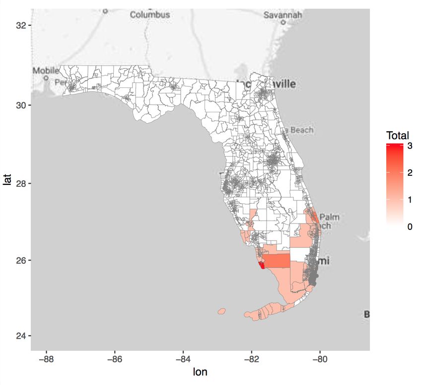
9Figure 2: Exposure to Hurricanes by Census Tracts, 1992-2017
Notes: This graph shows the number of times a census tract is within the radius of
hurricane-scale wind speed (64 nautical miles per hour) during 1992-2017. Cal-
culations are based on detailed hurricane track points and census tract population
centroid.
Hurricane damages rise exponentially with wind speed. We are thus interested in de-
termining exposure to Category-3-and-beyond hurricane wind speed (96+ kn or 110+ mph)
separately for heterogeneity analysis.16 Since maximal reach radius of 96 kn is not provided
in the dataset, we calculate our own measure by estimating a nonlinear relationship between
wind speed and its reach radius (see Appendix B.1 for details on this procedure and the
validity checks).
Throughout this paper, we define hurricane exposure by whether a location was ever
within the reach of a 64 kn wind speed radius along a hurricane path. Severe exposure is
similarly defined but with a 96 kn wind speed. This requires both proximity to the hurricane
16 We use the category 3 speed threshold both to be in line with previous literature, and because
we do not believe the difference between the categories 1 and 2 thresholds is sufficient to produce
measurable differences in outcomes. Category 4 wind speeds, on the other hand, almost never reach
Florida shores over our hurricane time period.
10Figure 3: Severe Exposure by Census Tracts, 1992-2017
Notes: This graph shows the number of times a census tract is within the radius
of category 3+ wind speed (96 nautical miles per hour) during 1992-2007. Cal-
culations are based on detailed hurricane track points and census tract population
centroid.
path and high sustained wind speed at that stretch of the path. The radius average 95 miles
for observations with wind speed above 64 kn, and 45 miles for those above 96 kn. It is
important to note that our exposure measure does not indicate actual damage. Houses lying
outside of hurricane-scale wind speed radius, for example, might also be affected by heavy
precipitation or flood, while those inside might sustain little damage due to strict building
code or high elevation. Rather, we use this measure to identify homes located in areas that
are likely to suffer from most direct impacts. Ultimately, we are interested in estimating
equilibrium adjustments in these areas rather than the impact of being damaged.
Figure 2 shows the geographic distribution of hurricane events by census tract, defining
exposure using their population-weighted centroids. Around 90% of tracts experience at
least one hurricane event between 1992 and 2017, with high variation in frequency across
locations. We plot the distribution of severe exposure events separately in Figure 3. This set
11of locations is much more limited (16%) and mostly concentrated in south Florida. The av-
erage census tract experiences 2.6 hurricane events and 0.16 severe exposure event between
1992 to 2017.
2.3 Home Mortgage Disclosure Act
The Home Mortgage Disclosure Act (HMDA), enacted by Congress in late 1975, requires
all large financial institutions17 to disclose all of their home lending activity every year. The
loans reported are estimated to represent about 80 percent of all home lending nationwide.
These records are made publicly available in an effort to improve home financing market
transparency.18 The HMDA data provides the date, property location (census tract), mort-
gage loan amount, purpose of application (purchase, improvement, or refinancing), mortgage
lender’s name and applicant demographics including annual income, gender, and race.
We merge the subset of successful loan applications for purchases from HMDA to our
transaction data following the matching procedure described in Bayer et al. (2016). Matches
are based on the year of each transaction, the census tract of the home, the loan amount (in
1000s), and the lender name.19 The full procedure ultimately matches just over half of the
original Zillow borrowers data, with no significant yearly variation in pairing success. This
match rate is similar to that in Bayer et al. (2016), which merges HMDA data to the universe
of housing transactions in the Bay Area. The merged data enables us to look at the evolution
of borrower demographic characteristics following hurricane events.
3 Econometric Framework
This section presents our research design. The first part of our analysis concerns post-
hurricane adjustments in the housing market. We study two main outcomes that characterize
the equilibrium – housing price and transaction probability – and use a separate regression
model for each. The models differ in the dependent variable and the unit of analysis. De-
spite these outward differences, both essentially rely on the randomness of hurricane paths
17 Bycurrent definition, a large financial institution is one with more than $45 million in assets.
This threshold is subject to yearly revision.
18 See http://www.ffiec.gov/hmda for more details.
19 See Appendix C for more details on the matching procedure.
12and timing as the identifying variation. In the second part of the analysis, we use a similar
specification to the housing price model to examine the associated population turnover.
3.1 Housing Price Model
We model the transaction price of a home as follows:
10
X
log(P riceihmy ) = τ
βτ Hurrimy + γ 0 HouseChariy + δht + δhm + δhcy + ihmy (1)
τ =−6
where i denotes an individual transaction, h the housing type,20 m the month and y the year
of the transaction, and t and c the census tract and county in which the transaction occurred,
respectively.21 The unit of analysis is an individual transaction. log(P riceihmy ) is the log of
price in transaction i, which involves a house of type h and takes place in month m of year
τ
y. Hurrimy is a set of indicators specifying whether the transaction occurs τ years after the
house was exposed to a hurricane (τ = 0 refers to transactions in the first twelve months after
a hurricane, τ = 1 the next twelve months, and so on; a negative τ indicates the transaction
happens before the hurricane). HouseChariy is a set of house characteristics commonly
used in hedonic models and include lot size, structural age, effective age,22 number of stories
and number of bathrooms. We control for the latter two characteristics flexibly using a set of
value bins. These variables are taken from an assessment in the year of the transaction. For
a given parcel, these variables might not remain the same over time and will be reflected in
the data if the home is transacted multiple times.
We also account for both fixed and time-varying regional differences in housing attributes
and local amenities by using a rich set of fixed effects. δht is type-by-tract fixed effects,
which absorb cross-sectional correlations in the likelihood of being hit by a hurricane and
time-invariant local amenities, such as proximity to the coast. δhm is type-by-month fixed
effects that control for the seasonality in both home prices and the timing of hurricanes.
It is also important to account for the housing booms and busts during our sample period,
20 We group homes into six main housing types based on land use classification in county tax
assessments. They include single family residential (68.3%), condominium (21.7%), townhouse
(6.83%), residential-multifamily (2.61%), vacation home (0.14%) and miscellaneous (0.4%).
21 Census tracts and counties are defined according to the 2000 census definition throughout to
maintain geographic consistency across time.
22 The time (in years) since the house last had a major remodel.
13especially given their uneven impacts across markets (Charles et al., 2017). We use type-by-
county-by-year fixed effects (δhcy ) to control for changing macroeconomic conditions at the
county level.
The key variables of interest are the hurricane indicators. They are constructed based on
the definition of hurricane exposure for individual parcels as described in Section 2.2.23 Their
identification requires that the idiosyncratic shocks to transaction prices are uncorrelated
with them:
E[imy × Hurriτ |HouseChariy , δht , δhm , δhcy ] = 0 ∀τ.
In essence, this is a staggered difference-in-difference (DID) framework with many hurri-
cane treatments at different times.24 Areas exposed to a hurricane are compared to unex-
posed ones before and after the hurricane in a repeated cross-section of housing transactions.
Intuitively, because hurricane paths and timing are exogenous, exposed and unexposed areas
are comparable absent the hurricane.
There are two main advantages of using this set of event time indicators rather than a
single indicator as in a standard DID specification. First, the post-hurricane housing market
might have transitional patterns that last an indeterminate duration. Analyzing these dynam-
ics can provide key insights into the market adjustment process. Our set of post-hurricane
indicators let them play out without imposing any restriction on the trend or duration. Sec-
ond, the pre-hurricane indicators also allow for full flexibility in the pre-trends. This provides
important evidence for us to assess the key identification assumption of DID, which requires
the treatment and control group to have parallel trends absent the treatment. Our speci-
fication allows for powerful detection of differential pre-trends and provides a transparent
partial test of the assumption.25 To sum up, we adopt a data-driven approach to minimize
misspecification and maximize the transparency of our research design.
Throughout this paper, we cluster standard errors at the county level to allow for corre-
23 Specifically, we calculate exposure to each of the 15 hurricanes for each transacted home. We
then construct the hurricane indicators based on the transaction timing relative to all hurricane events
the house is exposed to.
24 This design has been used by several studies of the economic impacts of natural disasters such
as Belasen and Polachek (2009), Strobl (2011), Gallagher (2014), Hsiang and Jina (2014), Deryugina
(2017), and Boustan et al. (2017)
25 In fact, Deryugina (2017) points out that the parallel trend assumption can be relaxed given the
exogeneity of the hurricane. See also Malani and Reif (2015). Our approach therefore provides extra
assurance on the validity of our identifying variations.
14lations in the idiosyncratic shocks to all transactions occurring in the same county over the
entire sample period. We also estimate four variants of it, as described below.
Repeat sales. Hurricanes might change the composition of transacted homes. Equation
(1) addresses this concern using a rich set of controls which greatly limits the extent of
composition shifts in the estimates. To further eliminate within-tract selection of transacted
attributes, we replace the census tract fixed effects with parcel-level ones:
10
X
1(T ransacted)py = τ
βτ Hurrpy + γ 0 HouseCharpy + δp + δhy + δcy + py . (2)
τ =−6
This approach restricts the identifying variation to price changes from repeated sales of the
same home and holds all time-invariant characteristics fixed. This method is used to generate
several major house price indexes26 and also widely adopted in academic research (Cannaday
et al., 2005; Hallstrom and Smith, 2005; Harding et al., 2007).
Wind intensity heterogeneities. We explore heterogeneous effects of different wind in-
tensities, as stronger winds bring much more severe damages to the housing stock. Specifi-
cally, we split the exposed areas into those under category 1-2 wind speeds and those under
stronger winds as discussed in Section 2.2. We estimate the dynamics of both groups simul-
taneously by interacting the indicator for each group with the event time indicators.
Other outcome variables. Hurricanes might change the set of homes transacted or the
type of home buyers. Understanding any systematic shift is important for us to assess the
nature of market responses to hurricanes. To do so, we replace the outcome variable in
Equation (1) with a given characteristic of interest, such as lot size or log income of the
buyer.
Standard DID. For ease of interpretation, we also estimate a standard DID model, defin-
ing treatment as being exposed to a hurricane in the last 36 months. The validity of this
specification can be inferred from results on the event study, as the identification assumption
is essentially the same for the two models.
26 Theseindexes include the Case-Shiller Index, Federal Housing Finance Agency’s (FHFA)
monthly House Price Index, and CoreLogic’s LoanPerformance Home Price Index.
153.2 Transaction Probability Model
A market equilibrium is characterized by both the price and the quantity. At the individual
home level, transacted quantity is either zero or one. Formally, let 1(T ransacted)py be
an indicator of whether a transaction record exists for parcel p in year y. We model its
relationship to hurricane events as follows:
10
X
1(T ransacted)py = τ
βτ Hurrpy + γ 0 HouseCharpy + δp + δhy + δcy + py . (3)
τ =−6
where p, h, y, and c denote parcel, housing type, year, and county as before. The unit
of analysis is now a parcel-year. We construct a balanced panel of most parcels that have
been transacted during the sample period. We treat all parcel-year observations without a
transaction record as having no transaction. This approach introduces measurement error
if there are unreported transactions, and can even lead to biased estimates if the missing
pattern is endogenous to or correlated with hurricane events. In our analysis, we take into
account detectable patterns of missing records in a few county-years by omitting these entire
counties from our sample. The combined sales in these counties account for less than 1%
of total sales as they are all small counties. Therefore, our approach of omitting the entire
sales histories does not yield any distinguishable differences in results from omitting only
the missing years. We also include only parcels that have been built before 2000, so that
the panel consistently tracks the housing stock that has been present at the beginning of the
study period. Florida is subject to tight land supply due to geographic constraints (Saiz,
2010). This endogenously generates strict zoning regulation and hinders new developments,
especially in dense urban areas.
We construct the panel by year rather than by month due to computational constraints.
As most hurricanes take place in August, many transactions in the same calendar year might
have happened before the hurricane. This will severely attenuate the estimate of the year
0 hurricane indicator if we define the event time based on the calendar year. Instead, we
redefine event years to begin in August and end in July. For example, a transaction in an area
exposed to Katrina (August 2005) will have its year 0 indicator turned on only if it occurs
between August 2005 and July 2006. This ensures a correct event year classification for
most transactions, an uncontaminated event year -1 indicator, and a small and predictable
16downward bias in the estimate of the event year 0 indicator.27
Despite the differences in the data structure, this model shares many similarities to the
previous one on housing price. We keep the same event-study specification. The model
also controls for time-varying house characteristics observed from repeated assessments.
Because the threat to identification is similar to that in the previous model, we also include
parcel fixed effects to isolate within-home variation, county-by-year fixed effects to control
for differential growth across counties, and type-by-year fixed effects for differential changes
in home types. The identification assumption is also similar:
E[py × Hurrpτ |HouseCharpy , δp , δhy , δcy ] = 0 ∀τ.
Our dataset includes three main parcel types: single family residence, condominium, and
townhouse. Due to limited substitutability between these types, their dynamics might be
different. Therefore, we also estimate this transaction probability model separately for each
type. The type-by-year fixed effects are eliminated in these estimations. The standard errors
are clustered at the county level throughout.
3.3 Variation in Hurricane Exposure
Hurricanes are rare events. Although their paths and timing are random, they might hit lo-
cations with distinctive characteristics and growth patterns by pure chance. This is an issue
discussed and explicitly accounted for in the past literature (Deryugina, 2017). We alleviate
this concern by using a longer hurricane history and hence a larger set of hurricanes. This
approach reduces small sample bias28 while preserving unbiasedness so long as hurricanes
are exogenous. It also allows us to maintain the interpretation of our results as the effects
27 Some hurricanes in our sample occur as late as October. The year 0 indicator might still get
attenuated because it captures some transactions in areas affected by these hurricanes right before
they actually took place. Given our approach to begin the year in August, this mechanical issue can
only affect transactions occurring in the three months preceding hurricane Wilma (October 2005) or
the two months preceding Frances and Jeanne (both dissipating in September 2004). The ensuing
attenuation bias to event year 0 indicator is small and predictable. An alternative is to begin the year
even later. However, this other alternative misclassifies some transactions of actually exposed homes
to event year -1. We choose to remove a few observations from the event year -1 group but keep it
uncontaminated: a future hurricane cannot have a causal effect on any of our outcomes before it hits
because its path is unpredictable.
28 “Small sample” refers to a limited set of hurricanes.
17of an average hurricane in Florida rather than a small, selected subset of hurricanes. From
Figure 2, we can see that Florida hurricanes during 1992-2017 create a fairly disperse geo-
graphic distribution together. In this section, we take a closer look at variation over time as
well as contribution by individual hurricanes.
For each separate hurricane, we first examine the percentage of transactions that are in
its affected area, in each of the 10 years before and after its occurrence (see Table A3 for
a summary of these percentages). Looking across hurricanes, we obtain a snapshot of the
composition of hurricane variations used in Equation (1), the housing price model.29 These
variation profiles illustrate that the seventeen-year width of our sample constrains the length
of pre- and post-hurricane dynamics that we can estimate in our models. Event years -5 to 10
all contain variation from at least ten out of sixteen hurricanes and 8-12% of transactions in
exposed areas. Event year -6 contain variation from six hurricanes and a total 5% impacted
transactions. However, variation in event years -10 to -7 come from only two hurricanes,
raising serious representativeness concerns.
We also generate similar variation profiles for Equation (3), the transaction probability
model (see Table A4). As this model is estimated using a balanced panel of parcels, the
exposed percentage is constant for each hurricane across event years. Again, we see a similar
pattern where earlier event years pick up variation from very few hurricanes, while event
years starting from -5 capture exposure to more hurricanes. In these later years, exposed
areas also account for around 10% of all parcels. Overall, these patterns attest to the similar
nature of identifying variation used in the two models.
Based on these patterns, we exclude indicators for event years -10 to -7 from the es-
timation. This leaves us with six pre-periods and ten post-periods, comparable to the past
literature that studies natural disasters using an event study design (Murphy and Strobl, 2010;
Gallagher, 2014; Gallagher and Hartley, 2017; Deryugina et al., 2018). We have also esti-
mated models with shorter dynamics and found the results robust in both direction and scale.
Lastly, we examine variation in severe exposure (category 3 or greater wind speeds) in
the same way (see Tables A5). The fraction of transactions subject to high wind speeds is
not only small (less than 1% in all years) but also limited to 5 hurricanes in total. This will
greatly limit the power when we estimate the heterogeneous effects of higher wind speeds.
29 The last row of each panel in Table A3 reports cumulative exposure in each event time year.
Note that this percentage is less than or equal to the sum of individual hurricane exposure because
transacted homes may have been hit by multiple hurricanes in an event year.
18In addition, the geographic concentration of severe exposure is high according to Figure 3.
This limited set of locations are less likely to have parallel pre-trends with the rest of Florida.
4 Results
The results are presented in several subsections below. We begin by estimating the post-
hurricane dynamics in housing prices for areas affected by hurricane while addressing poten-
tial composition effects in Section 4.1. Likewise, we estimate how transaction probabilities
adjust for parcels in these areas in Section 4.2. Together, these two outcomes characterize
equilibrium shifts in the housing market as it recovers from hurricanes, which we interpret
further in Section 4.3. In Section 4.4, we examine the implications of these market adjust-
ments on local population turnover. In Section 4.5, we explore whether the previous effects
are heterogeneous according to hurricane intensity.
4.1 Post-Hurricane Price Dynamics
We first estimate the post-hurricane dynamics of housing prices using the full sample of all
transactions. The average price and home attributes in these transactions are reported in the
first two columns in Table A1. We use a flexible difference-in-differences specification as
detailed in Equation (1). The standard errors were clustered by county over the entire sample
length.
The estimated coefficients of event year indicators are plotted along with their 95% con-
fidence intervals in Figure 4 (the full results are reported in the first column of Table A9).
None of the estimates for pre-hurricane indicators are statistically different from zero, sup-
porting our choice of fixed effects that control for preexisting differences in average census
tract prices, seasonality, and county-specific dynamics. Our event year 0 and 1 estimates
suggest that hurricanes result in increases in home prices of 5% in the first and 10% in the
second twelve-month periods after the strike. The surge in prices appears to end sometime in
the next twelve-month period (event year 2) as the estimated increase relative to unaffected
homes drops to 2% and is no longer statistically significant. All later event year estimates
are small and not statistically distinguishable from zero. In short, the estimates suggest a
temporary surge in prices in the three years immediately following a hurricane in exposed
19areas. In Table A6, we provide additional results using a standard DID specification, defin-
ing treatment as being in event year 0-2, for the overall market as well as by home types. The
main takeaway is, while there is an overall increase in home prices, the effect is particularly
pronounced for condominia.
One possible interpretation is a shift in the distribution of transacted homes: in the after-
math of a hurricane, homes with greater hurricane resistance, quality or general desirability
might be more likely to get transacted. In the extreme, the price surge could have been en-
tirely driven by such composition shift without actually reflecting change in any individual
home’s price. Our model partially addresses this possibility by controlling for a standard set
of hedonic variables. The estimated effect is thus free of a shift in observed quality or any
unobserved aspect that is strongly correlated with the observed characteristics.
Nevertheless, we cannot completely rule out this possibility due to limited observability
of damage-related house characteristics such as base elevation or roof condition. To inves-
tigate this issue further, we re-estimate our price model with the inclusion of parcel fixed
effects, and restrict the sample to only include homes which were transacted at least once
both before and after a hurricane. The result is plotted in Figure 5 and reported in the second
column of Table A9. The standard errors are slightly larger due to the extensive fixed effects
and a smaller sample size. On the other hand, this specification yields stronger evidence of
parallel pre-trends which suggests greater credibility in identification. More importantly, the
previous patterns are closely reproduced and if anything, larger in scale. Our point estimates
imply that these homes on average sold at 5% higher prices in the event year immediately
following the hurricane, as much as 14% in the next event year, and 8% in the third event
year. These results suggest that the homes sold in the first two to three years in exposed areas
appreciated relative to when they were sold outside of this post-hurricane window. More-
over, such within-home appreciation is likely to be the main driver of the price effect in the
full sample, given its slightly larger magnitude. In order to better understand the mecha-
nisms behind this finding, we now turn towards the potential hurricane-induced changes in
the probability of home transaction.
4.2 Post-Hurricane Dynamics of Transaction Probability
We estimate the post-hurricane dynamics of transaction probability using Equation (3). As
described in Section 3, we use a balanced panel of parcels where each observation is a parcel-
20Figure 4: Hurricane Effects on House Prices – Full Sample
.2
.1
Log Price
0
-.1
-.2
-6 -5 -4 -3 -2 -1 0 1 2 3 4 5 6 7 8 9 10
Event Time Years
Notes: Estimates from Equation (1) are plotted with their 95% confidence intervals. The
model controls for standard hedonic variables and census tract, month, and county-year
fixed effects. Standard errors are clustered by county. The results are based on the full
sample of Florida home buyers (N = 7,408,259).
Figure 5: Hurricane Effects on House Prices – Repeat Sales
.2
.1
Log Price
0
-.1
-.2
-6 -5 -4 -3 -2 -1 0 1 2 3 4 5 6 7 8 9 10
Event Time Years
Notes: Estimates with parcel, month and county-year fixed effects are plotted with their
95% confidence intervals. The model also controls for age and effective age at time of sale.
Standard errors are clustered by county. The results are based on only parcels with repeated
transactions appearing in both pre- and post-hurricane periods (N = 1,338,384).
21year with an associated indicator for whether or not a transaction occurred in that year. Our
analysis focus on only parcels with a structure built before 2000. The summary statistics are
reported in Table A2.
The estimates from the full sample are plotted along with their 95% confidence intervals
in Panel (a) of Figure 6 (as well as reported in the third column of Table A9). The standard
errors are again clustered by county over the entire sample length. Baseline probability of
transaction is around 10%. Again, we see a stable pre-trend with all pre-hurricane indicators
being statistically indistinguishable from zero. In event year 0, the estimate indicates a drop
of 0.9 percentage points, or nine percent of the baseline probability, which is also statistically
significant at the 5% level. The effect shrinks to 0.3-0.5 percentage points in the next three
event years, and gradually returns to the baseline.
There are three main types of parcels in this dataset: single family residence, condo-
minium, and townhouse. As shown in Table A2, their characteristics are quite different and
substitutability between them might be limited. Considering also the wide confidence in-
tervals for the above estimates, it is likely that these market segments might have different
equilibrium dynamics. Therefore, we also estimate the model for each type separately. These
results are reported in panels (b)-(d) in Figure 6.30
Single family residences are the largest segment of the housing market and make up
around 70% of all transactions. For them, we observe a negative but small effect that peaks
at 5 percentage point in event year 1, and none of the event year indicators is statistically
significant at the 5% level. In contrast, we observe larger changes in transaction probability
for the latter two types of homes. Condominia, which usually represent 20% of transactions,
are nearly 3 percentage points less likely to be transacted in event year 0, 1 percentage
points in the following two event years, and around 0.5 percentage point in the next, before
returning to the baseline. Townhouses make up the smallest share of the market at under
10%, and experience a drop of 1 percentage point in the first two event years.
Taken together, our results show a 6% decrease in transaction probability in the entire
market, averaged over three years. We provide a more direct display of these scales by home
type in Table A7, where we report estimates from a standard DID specification. The results
again show substantial heterogeneity: the effects range from a 20% drop for condominia to
only 3% for single family residences. We consider the potential sources of such heterogene-
30 We use the same specification except for dropping house-type-by-year fixed effects.
22Figure 6: Hurricane Effects on Transaction Probability by House Type
(a) All Parcel Types (b) Single Family Residence
.01 .01
Transacted = 1
Transacted = 1
0 0
-.01 -.01
-.02 -.02
-6 -5 -4 -3 -2 -1 0 1 2 3 4 5 6 7 8 9 10 -6 -5 -4 -3 -2 -1 0 1 2 3 4 5 6 7 8 9 10
Event Time Years Event Time Years
(c) Condominium (d) Townhouse
.02
.02
Transacted = 1
Transacted = 1
0 0
-.02
-.02
-.04
-.04
-6 -5 -4 -3 -2 -1 0 1 2 3 4 5 6 7 8 9 10 -6 -5 -4 -3 -2 -1 0 1 2 3 4 5 6 7 8 9 10
Event Time Years Event Time Years
Notes: The estimates from Equation (3) are plotted with their 95% confidence intervals. Stan-
dard errors are clustered by county. Panel (a) plots the results based on all parcel types (N =
49,120,139), panels (b)-(d) are based on single family residence (N = 33,651,628), condominium
(N = 12,836,476), and townhouse (N = 2,976,067), respectively. The model controls for effective
age, parcel and county-year fixed effects. In panel (a), the model also includes type-year fixed effects.
23ity in the next section as part of a discussion of mechanisms.
4.3 Mechanisms for Price and Transaction Probability Dynamics
In the previous two sections, we find that post-hurricane housing markets see an increase in
housing prices and a concurrent fall in transactions. These dynamics together are consistent
with a negative supply shock. We further find that this shock is temporary, as both price and
probability appear to respond for two to three years and eventually return to the baseline.
To clarify, this does not imply that hurricanes only induce supply-side adjustments. In
fact, localities exposed to hurricanes are likely to experience changes in housing demand
through mechanisms such as people updating their beliefs in local disaster risk (Bin and
Polasky, 2004; Hallstrom and Smith, 2005; Bin et al., 2008; Gibson et al., 2017), disrup-
tions to local industries and labor market (Belasen and Polachek, 2009; Seetharam, 2018),
among others. However, it is very hard to exhaust all possible factors in demand or supply
that might shift after a hurricane and estimate the magnitude of each. Instead, we remain
agnostic about them so far but choose to estimate directly the first-order effect driving the
market equilibrium. Below, we interpret these findings further by discussing the nature of
the negative supply shock and exploring a number of alternative explanations.
Mechanism 1: Physical damage and repair process.
Hurricanes generate extreme winds and severe flooding that can destroy or cause sufficient
damages to buildings. As a result, part of the housing stock in exposed areas becomes un-
inhabitable in the short run, which explains the negative supply shock. It also creates a
mechanical drop in the transaction probability because it is very hard to sell a house in a
damaged state. Affected homeowners may seek to temporarily relocate to habitable proper-
ties nearby through renting, which is covered by insurance companies and federal assistance
in most cases. Demand increases in the rental market, which, in turn, put upward pressure
on housing prices. This might partly account for the large price increase for condominia: a
larger percentage of them are rental properties and might see more appreciation.
It takes time for homeowners to restore their homes to the original condition. For one,
a large majority of affected homeowners seek post-hurricane financial relief in the form of
24insurance payment or FEMA assistance.31 This requires homeowners to go through the filing
process, wait for assessment of the damages to be performed, and settle potential disputes
with the insurance company. This process can take months because federal institutions and
private insurance companies are often overwhelmed by claims at times of large-scaled dis-
asters. The findings in Gallagher and Hartley (2017) directly shed light on the time frame
for households to obtain disaster aid: while victims of hurricane Katrina use disaster relief
to pay down home loans, the effect did not stabilize until after a year.
The rebuilding or repairing process can also take a long time. Anecdotal evidence sug-
gests that post-disaster recovery is often hindered by a shortage of construction labor. In the
end, most people find it takes at least 18-24 months to repair, rebuild, or replace their home
and possessions after a large loss. Notably, this duration is consistent with the observed
effects on price and and probability. In particular, according to the Florida Condominium
Act, the condominium association is responsible for repairing the exterior damages rather
than the homeowners. This division of responsibility could further restrict condo supply in
the market, which is also consistent with the particularly large effect in this market segment.
Overall, physical damage and destruction provides a plausible explanation that matches the
findings well.
Mechanism 2: Quality improvement through rebuilding.
Another possibility is that the rebuilding process not only restores but also improves the qual-
ity of the home, thereby driving up its value. This could happen for a number of reasons.
First, if the repair is funded by insurance payment or government assistance, the homeowner
has an incentive to overuse the construction service (e.g. to better account for the possibility
of future events through investment in more disaster-resistant structures and materials). Sec-
ond, the building codes in Florida have been updated multiple times over the sample period
largely for the purpose of enhancing resistance to natural disasters. The restoration project
might thus be subject to stricter codes compared to its original construction.32 Lastly, hur-
31 There are various types of financial relief homeowners can seek after a disaster. For exam-
ple, wind damages are often covered by homeowner’s insurance, while flood damages are separately
covered by flood insurance. Homeowners might also seek relief from the federal government for un-
covered damages through the Individual Assistance program (Kutz and Ryan, 2006; Michel-Kerjan,
2010; Hoople, 2013; Gallagher and Hartley, 2017; Deryugina et al., 2018; Kousky et al., 2018).
32 A 2018 report on new residential building codes and enforcement systems by the Insurance
Institute for Business & Home Safety gave Florida a rating of 95/100, the highest score among all the
states it evaluated.
25You can also read