2015 AASHTO Bottom Line Report - Transportation Bottom Line
←
→
Page content transcription
If your browser does not render page correctly, please read the page content below

|||||||||||||||||||||||||||||||||||||||||||||||||||||||||||||||

                                                  2015 AASHTO
                                             Bottom Line Report
                                                      EXECUTIVE VERSION

            Transportation Bottom Line

AMERICAN ASSOCIATION OF STATE HIGHWAY AND TRANSPORTATION OFFICIALS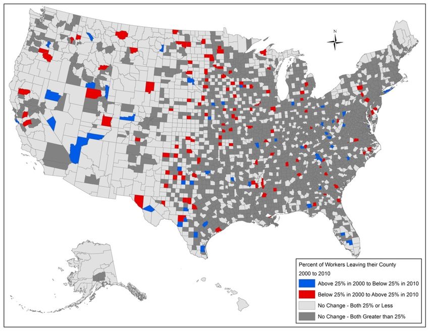
2015 AASHTO Bottom Line Report
                     Executive Version

                                Transportation
                                 Bottom Line

                               PREPARED FOR
                                  AASHTO

           Alan E. Pisarski                              Arlee T. Reno

The information contained in this report was prepared as part of NCHRP Project HR-20-24, Task 086,

National Cooperative Highway Research Program.

SPECIAL NOTE: This report IS NOT an official publication of the National Cooperative Highway Research

Program, Transportation Research Board, National Research Council, or The National Academies.

                                                  1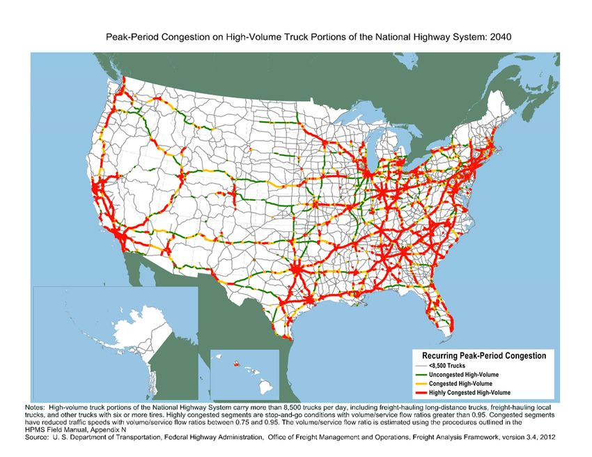
AT A GLANCE

An annual investment of $120 billion for highways and bridges between 2015 and 2020 is
necessary to improve the condition and performance of the system, given a rate of travel
growth of 1.0 percent per year in vehicle miles of travel, which has been AASHTO’s
sustainability goal, and which represents the likely impacts of both population growth and
economic recovery.

If travel growth is at 1.4 percent per year, which carries forward the rate employed in the 2009
Bottom Line and is consistent with the long term trend from 1995 to 2010, and has been
indicated in recent months, then needed investment to improve the highway and bridge system
will be $144 billion per year.

In 2010, the most recent year for which full data has been compiled by the Federal Highway
Administration, highway capital investment from sources other than the American Recovery
and Reinvestment Act, totaled $88.3 billion per year, but future funding levels are now highly
uncertain.

An annual investment of $43 billion for public transportation is necessary to improve system
performance and condition, given an expected 2.4 percent annual growth in transit passenger
miles of travel.

If transit ridership growth rises to 3.5 percent, the level that would double transit passenger
miles of travel in 20 years, investment in public transportation capital would have to increase to
$56 billion per year.

In 2011, transit capital investment from all levels of government totaled $17.1 billion, according
to APTA.

The model based investment estimates do not include all needs. Highway operations
investments, safety and security, and environmental mitigation costs for highways and transit

                                                2
capital projects may add over $10 billion per year to annual investment costs, although these
are not compiled for all systems and agencies. Importantly, long term highway reconstruction
costs may also not be fully captured.

The highway and bridge backlog required to restore the system to the level of condition and
performance required to meet today’s demand is $740 billion: of that amount the highway
system rehabilitation backlog accounts for $392 billion; the highway system capacity expansion
backlog accounts for $237 billion; and the bridge rehabilitation backlog accounts for $112
billion.

The highway system rehabilitation value of $392 billion plus bridges at $112 billion, is roughly
comparable in concept to the transit state of good repair (SGR) backlog approach, which has a
value of $77.7 billion. The FTA has not calculated a transit system capacity expansion backlog.

Recent research “A Failure To Act” sponsored by the American Society of Civil Engineers on the
economic impacts of investing to improve conditions and performance of highways and public
transportation indicated that the average US household will benefit by a cumulative $157,000
extra income between 2012 and 2040 compared to current levels of highway and transit
investment, which is more than three times current median household income.

An economic analysis for APTA of the transit investments in the 2009 Bottom Line report
showed that the marginal return from investing additional dollars in transit capital was 3.7
times the incremental cost of those investments.

FHWA’s condition and performance report for 2010 showed that by the end of the 20 year
analysis period, the annual user cost savings from higher levels of highway investment were 2.6
to 3.8 times as great as the annual added investment over current levels.

Between 1991 and 2011, both highway vehicle miles of travel and transit passenger miles of
travel increased at a long term average annual rate of 1.6 percent.

Highway travel declined during the recession and its aftermath, and has slowly resumed growth
since 2011, reaching an annual increase of only 0.6 percent in 2013 and transit travel grew only
1.1 percent in 2013, reflecting the slow beginning of the economic recovery from the great
recession.

Highway travel is expected to reach 3 trillion miles of travel again in 2014 not seen since 2008.

                                                3
In 2011, the freight transported in America was 17.6 billion tons, with 64 percent by truck, and
freight ton miles are expected to grow 72 percent from 2015 to 2040.

In 2013, transit passengers totaled 10.7 billion, the highest level since 1956.

International tourism, an intense user of our transportation system, generated $181 billion for
the US in 2013.

Transportation industries employ more than 11.7 million persons.

Since 1950, the population of the United States more than doubled but the road system grew
only from 3.3 million miles to 4.1 million miles.

The number of motor vehicles in the United States has quadrupled from around 65 million at
the start of the Interstate in 1956 to 254 million in 2012.

The overall population of the US is anticipated to grow by 37 million from 2010 to 2025, but the
over 65 population is expected to grow by 25 million, the under 18 population by 4 million, and
the working age population of 18 to 64 by only 8 million.

Structurally deficient bridges have declined by 43% from 1994 to 2013, but 63,500 SD bridges
remain.

Highway fatalities have decreased from 41,000 in 2007 to an estimate of below 33,000 in 2013.

                                                 4
ACKNOWLEDGEMENTS

This study was conducted for AASHTO with funding provided through the National Cooperative
Highway Research Program (NCHRP) Project 20-24 (086)]. The NCHRP is supported by annual
voluntary contributions from the state Departments of Transportation. Project 20-24 is
intended to fund quick response studies on behalf of the States.

This report is the product of cooperative research sponsored jointly by the National
Cooperative Highway Research Program (NCHRP) and the Transit Cooperative Research
Program (TCRP).

AASHTO and APTA provided both input information and source data, and AASHTO and APTA
staff have provided advice on what changes since the 2009 Bottom Line Report warrant
attention for this update.

Alan E. Pisarski and Arlee T. Reno, independent researchers, have served as the research team
for this report and were also the primary team members for the 2009 Bottom Line Report.

Ross Crichton, leader of the USDOT’s team for the 2013 Condition and Performance Report, and
many of his DOT colleagues have provided valuable inputs and advice on data sources and
analysis.

This effort was guided by the panel for NCHRP Project 20-24(86), with NCHRP staff support
from Dr. Andrew Lemer and Ms. Sheila Moore. The panel provided guidance on all aspects of
the project and advice and assistance on sources and methods.

DISCLAIMER

The opinions and conclusions expressed or implied are those of the researchers that performed
the research and are not necessarily those of the Transportation Research Board or its
sponsoring agencies. This report has not been reviewed or accepted by the Transportation
Research Board Executive Committee or the Governing Board of the National Research Council.

                                              5
NCHRP Project 20‐24(86), FY 2013
Critical Assessment for Future Surface Transportation Needs Analyses (Refresh the Policy
                            Capacity of the Bottom Line/C&P)

                                          6
MEMBERS
Mr. Don T. Arkle P.E.
Alabama DOT
Mr. Joseph Costello
Chicago Regional Transit Authority
Ms. Sharon L. Edgar
Michigan DOT
Mr. Ronald Epstein
New York DOT
Ms. Carolyn Flowers
Charlotte Area Transit Systems
Mr. Dan Franklin
Iowa DOT
Mr. Benjamin T. Orsbon, FAICP
South Dakota DOT
Ms. Elizabeth Presutti, AICP
Des Moines Area Regional Transit
Mr. John H. Thomas, P.E.
Utah DOT
Mr. Mark Huffer
Kansas City Area Transportation Authority
7FHWA LIAISON
Mr. Ross Crichton
AASHTO LIAISONS
Mr. Shane Gill
Dr. Matthew Hardy
APTA LIAISONS
Mr. Darnell Grisby
Mr. Arthur Guzzetti
NCHRP STAFF
Dr. Andrew Lemer
Ms. Shelia Moore
8FOREWORD
2015 will be a critical year for the future of America and for the surface transportation program.
Congress and the Administration will be called upon to craft legislation that will put in place the
surface transportation programs that will be essential to the nation’s economic recovery and
quality of life. The challenges of funding are arrayed against the overwhelming case that
enhanced investment is absolutely critical to the future of the nation.
Many issues must be addressed including but not limited to the following:
Investing in highway and transit infrastructure not only to sustain a recovery but also to support
long term economic success for all Americans.
Sustaining the solvency of the Federal Highway Trust Fund.
Maintaining rural and urban access and connectivity
Addressing transportation impacts on global climate change and climate change impacts on
transportation.
Reconstruction needs of an aging transportation system.
Reducing congestion on highways and crowding on major transit lines.
Increasing the capacity and safety of transportation systems.
Maintaining international competitiveness.
This comprehensive assessment of highway, bridge, and transit investment needs provides a
definitive base of information for decisions about levels of necessary investment. It is based on
the forecasting models and data systems used by the US Federal Highway Administration and
the US Federal Transit Administration, and on the results of FHWA analyses, supplemented by
additional research. The result is the most comprehensive analysis of the nation’s
transportation investment needs which is now possible.
9TABLE OF CONTENTS
AT A GLANCE 2
ACKNOWLEDGEMENTS 5
MEMBERS OF THE PANEL 7
FOREWORD 9
KEY FINDINGS 12
THE VALUE OF TRANSPORTATION INVESTMENTS 16
Transportation Employment 16
The Role of Tourism 17
Freight Movement 18
Rural Connectedness 20
A NEW ECONOMIC FOCUS FOR THE BOTTOM LINE 23
Global Competitiveness and Infrastructure 23
Evolution From Job impacts to Overall Economic Impacts 24
Project Economic Impacts- SHRP 2 Research 29
The Safety Benefits of Highway Investment 32
The Value of Public Transportation Investment 35
PRESENT AND FUTURE TRAVEL DEMAND 38
Where is VMT Heading 38
Harbingers of Recovery 43
Freight
Work and Work Travel Gains
Consumer Spending on Transportation Gains
Congestion “Gains”
The Future Travel Demand Structure 47
DETERMINING HIGHWAY INVESTMENT REQUIREMENTS 51
Highway Ownership and Condition 51
Bridges and their Condition 57
The Highway and Bridge Backlog – A Critical Concern 62
The Highway Backlog – Improving Estimates of Long Term Needs 66
The Bridge Backlog 67
A SCENARIO APPROACH TO HIGHWAY AND TRANSIT INVESTMENTS 68
10Need for a Scenarios Approach 68
Constructing 2015 Executive Bottom Line Investment Scenarios 70
How Highway and Bridge Scenarios are Constructed 70
How Transit Scenarios are Constructed 72
EXECUTIVE BOTTOM LINE 2015 SCENARIOS 73
Highway and Bridge Investment Scenarios 73
Full Employment Scenarios 74
Other Highway and Bridge Scenarios 75
Elements not Fully Included in Identified Investment Requirements76
Public Transportation Investment Scenarios 78
Public Transportation – The Bottom Line 79
Ridership and Passenger Miles of Travel 79
Public Transportation Services 80
Public Transportation Infrastructure 83
Transit Assets – Their Condition and Performance 83
Transit Infrastructure – the State of Good Repair 90
APPENDIX 93
11KEY FINDINGS
During the present period of recession and long recovery there has been an opportunity for
governments to “catch up” with road system and transit investment requirements as demand
growth has been limited and construction and rehabilitation costs were low. This,
unfortunately, has not been realized as federal, state and local government resources were
sharply limited during the same recession. As a result the backlog of national investment needs
for both rehabilitation and other condition improvements, and response to historical capacity
deficits remain substantial.
Highway and Bridge Requirements
Three primary highway and bridge investment scenarios were developed and evaluated, along
with their sub-scenario variations. These employ varying criteria and varying levels of expected
growth. Selected results important to gaining a comprehensive sense of national investment
needs are presented here.
Highways and Bridges Maximum Economic Investments
Maximum Economic Investment – ‐‐‐‐‐‐
Needed Spending per Year
Growth Rate of VMT per Year (Billions of Year 2012 Dollars)
Modal Comparison Scenario ‐‐ 1.6 Percent Annual Growth $156.5
Mid Level Scenario – 1.4 Percent Annual Growth $144.4
2009 BL Policy Scenario ‐ 1.0 Percent Annual Growth $120.2
At a 1.6 percent growth rate in VMT, called a Modal Comparison Scenario wherein both
highways and transit are shown at the same growth rate that each has averaged over the last
twenty years, annual average investment requirements for highways and bridges total $156.5
billion. In the Mid Level Scenario, at a 1.4% VMT growth rate, investment requirements are
$144.4 billion. Under a Policy Variant Scenario of nearly constant VMT/capita, at a 1.0 percent
annual VMT growth rate, the investment requirements decline to $120.2 billion.
12These scenarios represent a 13 percent and a 9 percent decline from the comparable 2009
Bottom Line scenarios which also used the growth rates of 1.4 percent and 1.0 percent. The 1.4
percent growth rate is consistent with the trend since 1995 and reflects judgments of recent
state estimates of highway travel growth.
The decline in investment needs from the 2009 Bottom Line is primarily due to the decline in
the FHWA’s cost index from 2006 (which was used in the 2009 Bottom Line) to the cost index in
2012 (which was used in the 2015 Executive Bottom Line). The cost index declined after 2006
but began to rise again after 2010 to the levels in 2012 and then moderated with only slight
change in 2013.
The Highway and Bridge Backlog
There has been a substantial expansion in the overall backlog of investment requirements for
Highways and Bridges, that amount needed to meet today’s need independent of future
growth prospects, as funding has failed to reach the necessary levels to sustain condition and
performance. At this time, given present lower construction costs, the investment required to
restore the system to the level of condition and performance to serve today’s demand is $740
billion: of that amount highway system rehabilitation accounts for $392 billion; highway system
expansion $237; and bridges $112 billion.
ARRA (the American Recovery and Reinvestment Act) funding has succeeded in making a
contribution to reducing those backlog deficiencies, not all of which have been fully tallied in
current reporting. The 2013 C&P (2013 Status of the Nation’s Highways, Bridges and Transit)
included spending under ARRA as current spending, but that spending had concluded at the
start of the Bottom Line analysis period for this study. Therefore this report estimates current
spending as the level of capital investment as developed by the 2013 C&P but excluding
spending from the ARRA. The current highway and bridge capital spending is at about $88.3
Billion per year under this updated definition.
A Full Employment Sub-Scenario
As part of these analyses it was recognized, given the key role that employment plays in travel
demand, that, while late in 2014 total national employment reached the levels that pertained
before the recession, the proportion of population at work has not reached the same levels
that had pertained prior to the recession. Thus, a scenario was developed for estimating the
travel effects of a return in 2015 to the previous share of employment (employment/population
13ratio) that applied before the recession. Such a level would add on the order of an additional
10 million workers in the society. Based on BLS consumer expenditure estimates of fuel
spending of workers vs non-workers an estimated incremental VMT level of 50 billion VMT was
derived as the added VMT for the enhanced or full employment scenario. This was treated as
an increment to the various VMT growth rates of the main scenarios.
It is worth noting that this estimate is a simple, straightforward illustration of the role that
employment plays resulting in direct changes to travel demand; it does not include estimates of
the second order effects in the economy of an added 10 million workers, which would be
substantial. It is also of interest that this estimate of full employment returns national VMT to
at least the levels that pertained pre-recession. Here in summary are the four scenarios of
maximum economic investment adding in the full employment increment to the 1.4 percent
regular scenario and to the 1.0 percent regular scenario.
Scenario At Base Level of At Full Level of
Employment Employment
$144.37 $148.17
Mid Level Scenario – 1.4 Percent Annual
Growth
Bottom Line Policy Scenario ‐ 1.0 Percent $120.17 $124.19
Annual Growth
Transit Investment Requirements
The economic growth or improve conditions, improve performance scenario for transit is
shown for three levels of growth in transit passenger miles. This scenario has traditionally been
referred to as “improve conditions, improve performance.” The table below illustrates the
average annual public transportation capital needs for the preferred scenario of improving
conditions and improving performance under the three different passenger miles growth
scenarios. In addition, to conform to FTA’s current practice in the 2013 C&P report, the cost of
only achieving a state of good repair (SGR) for current transit assets is also identified. The state
of good repair estimate is independent of passenger miles. The SGR estimate in the 2013 C&P
was $18.5 billion per year in 2010 dollars for reducing the backlog over twenty years, and this
estimate was adjusted to $19.1 billion for 2012 dollars to conform to the cost adjustments for
the other scenario estimates. The estimate used of current transit capital investment spending
is $17.1 billion for the year 2011, taken from APTA’s 2013 Fact Book.
14The three scenarios which constitute improve/improve at different growth rates are highlighted
as in recent Bottom Line reports. In addition, to conform to FTA’s current practice in the 2010
C&P report, levels of continuing current spending and the level of only achieving a state of good
repair (SGR) for existing current transit assets are also identified. These latter two are adjusted
from the 2013 C&P report results using cost index factors.
Public Transportation Capital Investments (Average Annual 2012 $ Billions) –
Levels For Current Spending, and Improve Conditions and Performance
Current Level
1.6 Percent 2.4 Percent 3.53 Percent
Annual Growth Annual Growth Annual Growth
Total Annual $17.1 $34.4 $43.3 $55.6
Needs
An Annual State of Good Repair (SGR) Estimate
The concept of State of Good Repair has been recently introduced in investment analysis. It
identifies what funding levels would be required to reestablish the entire system to a level of
what would be considered good condition or good repair. A highway and bridge State of Good
Repair (SGR) value is presented here, based on the SGR scenario included in the 2013 C&P
report, adjusted only for cost index changes. When adjusted, the comparable 2015 Bottom
Line estimate would be $83.1 billion per year. This should be considered to be an
approximation to be applied across all the different VMT growth rates. Pavement and bridge
damage will vary somewhat based on different heavy truck VMT growth rates, but these
analyses have not been done for the 2015 Bottom Line and so the SGR numbers are shown as
the same for the alternative VMT growth rates. Absent a full national survey these estimates
are not able to include a comprehensive national need for full future reconstruction of the
aging Interstate and other facilities.
A parallel value for SGR for transit amounts to 19.1 Billion based on an adjusted cost for 2012
compared to the 2010 costs in the latest C&P. As in highways and bridges this value is
independent of capacity needs.
15THE VALUE OF TRANSPORTATION INVESTMENTS
TRANSPORTATION EMPLOYMENT
As of 2012 the nation’s transportation-related labor force stood at 11.7 million workers, just
under a 9% share of total national employment. Those numbers are down from the peak at the
start of this century of 13.9 million transportation workers and a 10.5% share of employment.
The largest component of that is the transportation and warehousing occupational group which
has remained relatively stable at 4.4 million throughout the period. Some of the main
occupational groups include:
MAIN TRANSPORTATION OCCUPATIONS 2012
Occupational Group Number
000’s
Truck Transportation 1,351
Urban Rural Intercity Bus Transit 96
Freight Transportation Arrangement 183
Couriers and Messengers 533
Warehouse and Storage 682
Transportation Equipment Manufacturing 1,456
Highway Street and Bridge Construction 292
Motor Vehicle and Parts Dealers 1,732
Gasoline Stations 841
Automotive Equipment Rental and Leasing 173
Travel Arrangement and Reservation Services 193
Ambulatory and Health Care 266
Automotive Repair and Maintenance 830
Parking Lots and Garages 119
Postal Service 611
USDOT 58
State and Local Government (2011) 834
Source: BTS, USDOT – categories identified by BTS
It is clear from this how substantial the nation’s dependence is on a properly functioning road
transportation system and the services that operate over it such as transit, trucking, couriers
and the postal service. Of major importance is the substantial role of freight movement in our
employment and economy. Other public vehicle operations beyond transit are also critically
affected by the state of the system including police, fire and other emergency services vehicles,
and the military.
16THE ROLE OF TOURISM
Although rarely specifically recognized, the United States is number one in the world in
revenues received from international visitors, as of 2012. In 2013, spending by international
visitors to the United States reached $180.7 billion. Of this, $41 billion consisted of purchases
by foreigners of US air carrier services and $140 billion was expended within the United States.
This generated a major trade surplus of over $57 billion in 2013. The US has benefited from
such a surplus in travel since 1989. This places tourism at 27% of all services exports in 2013,
and places it ahead of exports of motor vehicles or of agricultural goods. Both domestic and
international transportation services are a key part of attracting and serving visitations. An
important shift has occurred in the visit arrangements of rapidly growing number of Asian
visitors in particular. This shift has been toward independent vehicle travel rather than the
group travel of earlier times. Both will see important growth in the future.
Consistent with the revenue increase, the US registered a record number of international
visitors in 2013, at just below 70 million visitors. Visitations have increased significantly each
year since the recession year of 2009 when 55 million visitors were counted. Significantly for
transportation concerns, the National Travel and Tourism Office forecasts a 20% increase in
visitors by 2018, reaching almost 84 million, equivalent to about an addition of 25% to the total
US population.
Prodigious as that number is, international visitors are a relatively small part of overall US travel
and tourism, although significant in financial terms. While only 4% of total tourism travelers,
they account for 17% of total tourism travel demand. They accounted for 15% of all tourism
highway tolls and 3% of all tourism gasoline consumption according to the NTTO. Historically,
they have been a significant part of car rentals, intercity bus and rail, as well as local transit and
taxis.
The overall travel and tourism industry in the United States is a major factor in the US economy
with total tourism-related employment at the end of 2013 in excess of 8 million, as estimated
by the Bureau of Economic Analysis in their Travel and Tourism Satellite Account. One million
of that employment is in transportation-related industries, not including air transportation
services. In the fourth quarter of 2013 the BEA placed tourism-related spending at $1.5 trillion.
According to the US Travel Association total domestic person trips of over 50 miles, reached a
low of 1,900 million, during the recession, but are expected to reach 2,160 million person trips
in 2016. Of this travel, about 22% is considered business-related travel and the remainder is
leisure and personal travel. A resurgence in the intercity bus industry with low cost carriers as
well as traditional tour-based activities is highly dependent on an effective road system.
17FREIGHT MOVEMENT
Of the almost 17.6 billion tons shipped in 2011, about 64% were shipped by truck. In addition,
trucks were heavily associated with multimode shipping and air and truck combination
shipments. This added approximately another 10% to the truck related share. When
shipments are examined in terms of their value, the total, including truck only, multimode
shipping and air and truck combination shipments rises to 88% of the almost $17 trillion of
goods shipped. The Figures below exhibit the patterns.
MODAL SHARESOther
OF TONNAGE 2011
Pipeline 2%
9%
Multiple
Modes Air and
9% truck,
Truck
0%
64%
Water Rail
5% 11%
MODAL SHARES OF SHIPMENT VALUE
2011
Other
Pipeline
5% 2%
Multiple
Modes
18%
Air and Truck
truck, Water 63%
7% 2% Rail
3%
A recent study was conducted by the ATRI (American Transportation Research Institute) on the
cost of congestion to the trucking industry. The study is based on billions of GPS data points of
truck flows drawn from a sample truck fleet of half a million vehicles throughout the country. It
sets that cost at $9.2 billion per year in increased operational costs as the result of 141 million
18hours of lost productivity in the national truck fleet. National trucking related congestion costs
in 2013 now range at around an average of $2.5 billion per calendar quarter. Many long-haul
trucks, which may cover 150,000 miles per year, experience an average added annual cost as a
result of congestion of over $5,000. ATRI calculates that 89% of costs occur in urban areas.
Costs per interstate mile among the most heavily congested states reach averages of a quarter
million dollars per mile.
The US DOT forecasts that freight movement will show substantial growth over the next 25
years in all freight elements, particularly in trucking. The current patterns and forecasted
trends are depicted in the figure below which shows the key components of trucking freight:
tons moved; ton-miles carried; and total value of goods moved. The FHWA forecasts indicate a
47% increase in tons in the 25 years from 2015 to 2040; ton-miles are expected to increase by
72%; and value by over 90%. This indicates substantial increases in average trip length and in
the average value per ton of goods moved. Increasing value places even greater importance on
timely movement and control of the logistics of the movements. Overall it represents a
dramatic challenge for the national road system. These values are for truck-only moves. Even
greater growth is forecasted for combined air and truck movements; and for mail and multiple
modes movements, in which trucking plays very prominent roles. The value of air and truck
movements are forecasted to more than triple between 2015 and 2040; and the mail and
multiple modes categories are forecasted to grow 2.7 times in the same period. As a result
there are very few freight moves in which trucking isn’t the sole or very crucial part.
TRUCK ACTIVITY TREND
30000
25000
20000
milllion Tons
15000
Billion Ton-Miles
10000 Value Billion$
5000
0
2007 2011 2015 2020 2025 2040
Source: Freight Facts and Figures 2012, US DOT, FHWA
19Even in international moves where air and water are the major factors, truck movements are
substantial. In addition to supporting many air and water moves with Canada and Mexico, our
number one and three international trade partners, with rapid trade growth trucking accounts
for almost 60 percent of moves across our borders, with the total value of trucking trade with
Canada and Mexico at the level of over two-thirds of a trillion dollars in 2013 according to BTS
statistics. The value of such trade grew by 50% between 2004 and 2013.
As a result truck congestion on already crowded long distance routes is expected to increase
substantially. The adjacent map below depicts the forecasted patterns of congestion in 2040.
RURAL CONNECTEDNESS
The history of the Nation has been inextricably tied to its ability to overcome the tyranny of
distance. America is a vast country in geographic extent, in population, in economic power and
technological capabilities. Few nations combine those four characteristics as we do. At the
same time it is a sparsely populated nation with extremely low average densities and vast
distances to traverse to meet the nation’s needs and support the well-being of its population.
20At least in potential, it has among the best connected rural populations in the world. The
combination of an extensive transportation system and high levels of communication, including
radio, television, telephone and internet connections provide the potential for high levels of
access to information and services and connection with the larger society. However, the nation
will need the full participation of rural populations in the economy and the society more than
ever in the future. Among the keys will be:
Access to agricultural products
Access to manufacturing facilities
Access to natural resources
Access to cultural and recreational opportunities such as National Parks
Access to viable retirement communities with the medical and other services requisite
for the aging.
But most of all it will be the resource represented by a well-educated rural population,
depending on definitions amounting to on the order of 50 million persons, that the nation will
need to integrate fully into the future economy in order to meet the nation’s requirements for
skilled workers.
As it is, of the 20 million workers living in rural areas, more than 3 million each day leave rural
areas for metropolitan jobs, and notably, the rural areas receive in return almost 2 million
workers from metro areas. The predominant flows are the very substantial flows within rural
areas within and between micropolitan centers, small urban clusters of between 10,000 and
50,000 population defined by the Census, that are emerging centers of economic activity.
About 10 million of the rural workforce live and work in these micropolitan areas. About 6.3
million work within their own rural non-micro areas and another 1.3 million flow between
micropolitan areas. These 20 million workers represent a great national resource who can
make even greater contributions to national GDP with expanded access to job opportunities.
While there has been a net decline in overall rural populations in recent times, there are, in
fact, substantial flows of new households from suburbs to rural areas (240,000 in 2011) and
from central cities (206,000), and directly from abroad as well. These indicate that there are
strong incentives and preferences for the rural life style among many.
It is critical to expand transportation capabilities to more effectively integrate rural capabilities
into the national structure for the sake of the nation’s rural population, and for the sake of a
greater national productivity and coherence. The nation cannot afford to have a large segment
of its population isolated from the economic opportunity and support services they require.
21Our transportation system must meet the test of providing greater access and connectivity to
this population.
22A NEW ECONOMIC FOCUS FOR THE BOTTOM LINE
GLOBAL COMPETITIVENESS AND INFRASTRUCTURE
The World Economic Forum produces a Global Competitiveness Report that helps identify the
roles that infrastructure plays in world competitiveness. The rankings are based on 12 pillars of
competitiveness grouped into three broad sub indexes:
#1 Basic Requirements;
#2 Efficiency Enhancers; and
#3 Innovation and Sophistication Factors.
Infrastructure is Pillar number 2 of 4 in the Basic Requirements Subindex as shown below:
Pillar one. Institutions
Pillar two. Infrastructure
Pillar three. Macroeconomic environment
Pillar four. Health and Primary Education
The key transportation elements of the Infrastructure Pillar, with their US rank for each, are
shown below:
Rank Elements of the Infrastructure Pillar US Rank
Country Rank
Germany 3 2.01 quality of overall infrastructure 19
France 4
2.02 quality of roads 18
Switzerland 6
Netherlands 7 2.03 quality of railroad infrastructure 17
United Kingdom 8 2.04 quality of port infrastructure 16
Japan 9 2.05 quality of air transport 18
Spain 10 infrastructure
Korea 11
2.06 available airline seat kilometers 1
Canada 12
Taiwan, China 14
United States 15
Inadequate supply of infrastructure is listed among the most problematic factors for doing
business in the United States. All US transportation infrastructure quality elements are
uniformly poor ranging from 16th to 19th in the world. The only service-level statistic, available
airline seat miles, stands out in terms of its top rank.
23The structure and mechanisms employed by the world economic forum have pertinence here
because they form a large part of the guidance that informed the US Chamber of Commerce’s
Transportation Performance Index first released in 2010. In another recent study by the
McKinsey Global Institute1 aimed at increasing the productivity of infrastructure investments,
the US is calculated to be investing at a rate of 2.6% of GDP; whereas, based on their estimate
of needs for all infrastructure investment derived from international norms and expected
national economic growth rates, the US ought to be investing at a level of 3.6% of GDP.
EVOLUTION FROM JOB IMPACTS TO OVERALL ECONOMIC IMPACTS
Assessments of the economic development effects of transportation investment have been
limited in past years. Many past assessments, often keyed to periods of economic stress,
tended to place focus on near-term job creation generated by the immediate stimulus to
construction work and materials production. These assessments often failed to account for the
longer term effects of improved travel times and access to opportunities afforded by new
transportation investment. Limited evaluation of the effects of transportation investments via
Before/After Studies may have missed the opportunity to demonstrate both the near-term and
longer term effects of major investments. The recent recession and slow growth aftermath has
aroused greater interest in ascertaining the linkages between highway investment and other
forms of transportation investment on overall long term economic development.
More and more attention is now being given to utilizing transportation investment to improve
the economic well being of households, businesses, and the nation as a whole. Benefits
assessed include both short and long term changes in employment, household and business
income, land values, and the improvements in access to workers, jobs, suppliers of materials
and services, and potential customers. Recent analyses for all modes have provided evidence
of the substantial long term economic benefits of additional investments in highways and public
transportation. Several of these analyses have analyzed the investment scenarios from the
previous Bottom Line or the previous Condition and Performance Reports. The newer analyses
have also extended economic analyses beyond the topic of user benefits to the consideration of
the overall economic impacts of investments on household income and business income.
The analyses of user benefits included in recent Condition and Performance reports provide a
starting point for the broader consideration of economic benefits. Both the 2010 C&P report
and the 2013 C&P report included sensitivity analyses which developed estimates of the user
1
Infrastructure Productivity, McKinsey Global Institute, Jan 2013
24benefits of increments of highway capital investment and increments of transit capital
investment. The 2010 C&P included a particularly detailed development of incremental
benefits from additional investments in highway capital projects. The table below shows the
results of the 2010 C&P sensitivity analysis of annual benefit cost ratios by the twentieth year of
investment for various levels of incremental annual investments in highways, developed from
analyses using the FHWA’s HERS model. It should be emphasized that this example shows a
calculation for only the HERS-modeled portion of highway investments which is related to the
federal aid highway system.
The results show very strong annual streams of benefits in relation to annual costs. Because the
HERS model chooses projects based on benefits versus costs, successively higher and higher
levels of investment in the HERS model result in successively lower and lower average ratios of
the total incremental benefits to the total incremental costs, simply because a rational system
invests in the highest pay-off projects first. However, total benefits still increase at a rate faster
than total costs, and very strong returns are shown at all levels of capital investment.
Incremental User Benefits From Added Highway Capital Investment
HERS Analyses for the 2010 Condition and Performance Report
Level of Annual Increment of Annual Increment of 2028 Ratio of 2028 Added
Investment as Investment Over Base Annual User Cost User Annual Cost
Modeled by HERS Case Investment Savings Over Base Savings to Added
(Billions of 2010 $) (Billions of 2010 $) (Billions of 2010 $) Investment
$54.7 (baseline) NA NA NA
$58.0 $3.3 $12.6 3.8
$62.9 $8.2 $29.9 3.6
$74.7 $20.0 $66.0 3.3
$80.3 $25.4 $79.7 3.1
$93.4 $38.7 $109.5 2.8
$105.4 $50.7 $132.0 2.6
Source: 2010 Status of the Nation’s Highway ‘s, Bridges, and Transit: Conditions and
Performance, and additional calculations.
25These results are also confirmed by more limited numbers of incremental investment analysis
done for the 2009 Bottom Line and for the 2013 Condition and Performance Report. Since the
highway construction cost index declined modestly from the time of the 2010 C&P until now,
and since the cost factors for benefits have increased modestly until now due to inflation of
consumer prices, the ratios of benefits to costs are now somewhat higher. Additional evidence
of the strong returns from highway investments have been developed in research for the
United States Chamber of Commerce, which showed that there were net benefits that more
than “paid back” the additional investment in a short period of time, even with cautious
assumptions that benefits would not accrue until several years after an investment.
Similar analyses have been done for incremental investments of transit capital, and similar
results are shown in the tables included in the sections of this report focusing on transit capital
investment. Other recent economic analyses of highway and transit investments, including the
Chamber work and research by the Economic Development Research Group for the American
Society of Civil Engineers, have extended these economic studies to include both user benefits
and broader economic benefits.
The broader economic analyses strengthen the results of the user related analyses in the more
recent 2010 and 2013 Condition and Performance reports. The set of studies conducted by
EDRG for the American Society of Civil Engineers (ASCE) covers all types of infrastructure. This
enables some comparison between investment in highway and public transportation systems
and investment in other types of infrastructure. Most interestingly, the studies utilized the
HERS and TERM model frameworks for analyzing highway and transit capital investments and
for estimating the funding gaps.
The table below shows the shortfalls by type of infrastructure that were estimated in the EDRG
study. The largest shortfall is in surface transportation. The shortfall was estimated by
comparing expected funding to needs, which for surface transportation were based on the
results of the analysis using HERS and TERM. The study forecasts of revenues for each
infrastructure category were based on existing sources of revenue for each category. The
surface transportation funding gap between 2012 and 2020 is estimated at $846 billion and by
2040 is estimated at $3,664 billion. In each case, the gap for surface transportation represents
the majority of the gap for all infrastructure categories combined: 77 percent of the total gap
by 2020 and 78 percent of the total gap by 2040.
26Failure To Act Report ‐ Funding Needs, Expected Funding, and
Shortfalls By Infrastructure Category ‐ Cumulative Amounts By Year
2020 and Year 2040 (All Amounts in Billions of 2010 Dollars)
2020 2040
Total Expected FundIng Total Expected Funding
Need Funding Gap Need Funding Gap
Surface Transportation $1,723 $877 $846 $6,751 $3,087 $3,664
Water/Wastewater $126 $42 $84 $195 $52 $144
Electricity $736 $629 $107 $2,619 $1,887 $732
Airports* $134 $95 $39 $404 $309 $95
Inland Waterways
& Marine Ports $30 $14 $16 $92 $46 $46
Totals $2,749 $1,657 $1,092 $10,061 $5,381 $4,681
The economic consequences of the infrastructure funding gaps are shown in the immediately
following tables which show the impacts on households and businesses by 2020 and 2040. By
2020, the shortfalls have caused a net loss for businesses and households as shown in the
tables just below. The net loss is after subtracting out what the businesses and households
would have paid as part of the investments made in infrastructure, so these amounts represent
unnecessary and undesirable net losses which cannot be recovered.
Failure to Act: 2020 Cumulative Losses ($2010 B)
Infrastructure Systems Households Businesses Total
Surface Transportation $481 $430 $911
Water/Wastewater $59 $147 $206
Electricity $71 $126 $197
Airports N/A $258 $258
Inland Waterways & Marine Ports N/A $258 $258
Totals $611 $1,219 $1,830
Note: Costs do not include personal income or value of time other than business travel.
For 2020, 79 per cent of the net losses are due to the surface transportation funding gap, which
is shown in the table above, and about 50 percent of total losses to households and business
are due to the surface transportation shortfall. The surface transportation category includes a
27small portion of intercity rail investment but the vast bulk of this is highways and public
transportation. For 2040, household losses are 66 percent due to surface transportation
shortfalls, and 34 percent of all losses are due to surface transportation shortfalls. These are
extremely conservative estimates of the negative consequences, despite how deleterious the
impacts shown are. Some of the impacts on households are missing for the other infrastructure
categories since no personal income effects are included.
Failure to Act: Cumulative Losses 2040 ($2010 B)
Infrastructure Systems Households Businesses Total
Surface Transportation $1,880 $1,092 $2,972
Water/Wastewater $616 $1,634 $2,250
Electricity $354 $640 $994
Airports N/A $1,212 $1,212
Inland Waterways & Marine Ports N/A $1,233 $1,233
Totals $2,850 $5,811 $8,661
Note: Costs do not include personal income or value of time other than business travel.
Same here
The table below shows the impacts on households as per household impacts on an annual basis
and amounts which are cumulative through 2010 and 2040. Since 79 percent of the impacts on
households by 2020 is due to the shortfall in surface transportation, the impact of the surface
transportation shortfall per household is a cumulative loss of $22,400 per household through
2020. Since the loss per household by 2040 is 66 percent due to the surface transportation
shortfall, the loss per household due to the surface transportation shortfall is $103, 800 per
household. Median household income in 2010 was just below $50,000, so these total losses
from a failure to invest in surface transportation for every household are equal to half of a
median household’s annual income by 2020 and equal to twice a median household income by
2040.
Failure To Act: Net Impacts Per Household
2012‐2020 2021‐2040 2012‐2040
Average Annual Disposable Income Per Household – $3,100 – $6,300 – $5,400
Total Disposable Income Per Household – $28,300 – $126,300 – $157,200
Note: Dollars rounded to nearest $100. Totals may not multiply due to rounding.
Sources LIFT/Inforum Model of the University of Maryland, and EDR Group.
28PROJECT ECONOMIC IMPACTS: SHRP2 RESEARCH
There is also a large and growing body of work which provides examples of the impacts of
investments in projects of various typologies. The second Strategic Highway Research Program
(SHRP2) has developed several products. A recent product of SHRP 2 Capacity Research2
assembled effective case studies of the impacts on economic and land development of highway
projects across a broad spectrum of types and situations. The study compiled before-and-after
information on 100 case studies in 10 different categories of investment in various geographic,
social, and economic settings with a set of observations balanced by region of the nation.
Of the 100, positive benefits were identified in 85 in the five year retrospective as elaborated
below. It was noted that in some cases longer term effects need to be recognized as well as
more immediate effects, especially for major facilities, that occur at sites far distant from the
facility.
Project Type Total Cases
Beltway 8
Bridge 10
Bypass 13
Connector 8
Interchange 12
Industrial access road 7
Major highway (limited access route) 14
Widening 9
Freight Intermodal Terminal 10
Passenger Intermodal Terminal 9
Total 100
The selection criteria included projects, greater than $10 million in cost, which represented new
highways, or major extensions, expansions, or other significant performance enhancement to
existing highways. Only facilities more than five years old were considered to give economic
development potential sufficient time to exhibit effects. A key factor was the project
2
Report S2-C03-RR-1; Interactions Between Transportation Capacity, Economic Systems, and Land Use, EDRG et
al, SHRP2@, TRB, 2012
29motivation by project type. Of the 97 projects reporting motivation, 58 identified an access
issue, 54 a congestion management issue, and 65 an economic development issue. The
distribution of project motivations by urban and rural locations is shown in the figure presented
later in this text. (In some cases multiple motivations apply).
It is often the case that major surface transportation investments are assessed in terms of the
jobs created by the investment, especially during economic downturns. While this was covered
quite effectively, broader impacts, such as income, business output building development,
direct private investment, property values, and property tax revenues were assessed. Of the 15
projects that showed zero or negative job impacts other benefits were identified: eight of the
cases showed gains in business sales; 10 of the cases demonstrated local per capita income
increases; and six documented property value increases. The one area which demonstrated net
negative job impacts was in the case of two bypasses studied. This was expected given the
positive and negative trade-offs inherent in such investments in the near term.
The study employed a job impact ratio to assess project effects. Overall the case studies
indicated a median ratio of seven long-term jobs generated per million dollars of highway
investment. The distribution of job impacts was very broad by type of investment; access roads,
interchanges and connectors tended to have the highest average ratios as shown in the figure
below.
Long Term Jobs Impact per Million
Invested
100
metro/mixed Rural
80
60
40
20
0
Many of the projects which show limited job generation per project are those of a major scale
such as beltways or major interchanges where the economic effects are often interstate and
inter-Metropolitan. Their major roles are often providing access to job opportunities or freight
30logistics benefits. Metropolitan investments generate more substantial job returns than rural
investments in the studies. Many of the rural investments are in the category of providing for
job benefits in areas far distant than the proximate construction area, or are in the category of
requiring longer periods to fully develop. It is notable that 66% of the metro level investments
identify long-term job growth impacts exceeding 1000 jobs.
The study also identified significant motivations for projects which can be a guide to future
economic development planning. The following figure shows the distribution of motivations for
the highway projects3. The graphic is notable not only for the rich information but also the
broad array of motivations that generated the highway projects. The key frequently is access to
other transportation facilities and international borders, as well as access to markets, and to a
broader labor force. Developments at specific sites, such as tourism venues, are highly
significant to rural areas studied. It is notable that mitigation of congestion is a significant
factor in both metropolitan and rural areas.
Project Motivations
57%
60% 52%
55%
52%
Metro Rural
50%
38% 39%
40% 32%
30%
30% 25%
21%
17%
20%
9% 9% 10%9% 9%
10% 5%
0%
The study makes the distinction between point-to-point projects and continuous roadway
projects. It is often the point-to-point projects which create access to industrial parks, office
parks and other industrial sites and therefore show demonstrable direct and immediate
benefits, whereas continuous roadway projects may generate important job effects hundreds
of miles away – – no less important, but more difficult to pinpoint.
3
Multiple motivations apply so numbers will not add to 100%
31THE SAFETY BENEFITS OF HIGHWAY INVESTMENT
NHTSA Study -- In a recent report4 NHTSA placed the 2010 economic costs of motor vehicle
crashes at $277 billion, based on the 32,999 fatalities in that year. Approximately a third of that
cost was the result of lost work place and household productivity and congestion costs
accounted for another 10%. About 9% of those costs were incurred by governments.
Roadway Safety Guide – A related report5 addresses the interaction between roadway design
and condition and roadway safety focusing on that portion of overall highway safety that is
determined by the roadway’s physical features, and surrounding environment. The report
indicates that nearly 53% of fatalities on America's highways occur in crashes in which the
condition of the roadway is a contributing factor. From an economic point of view just the
economic cost of these crashes is greater than three times the annual investment by all levels
of government nationwide in roadway improvements. This, of course, does not include the
distress, personal losses and social dislocation generated by such crashes.
The Guide describes some of the cost beneficial crash countermeasures and design strategies
that have been shown to be effective in reducing the number and/or severity of highway
crashes as shown below:
Crash Countermeasures Potential Effects
relocate roadside objects Reduce fatal or injury crashes 64%
install median barriers Reduce fatal or injury crashes 88%
Construct roundabouts Replacing signalized intersections reduces
crash 35% and fatalities by up to 90%
rumble strips Reduces drift off road crashes by up to 80%
timely ice and snow removal Restoring friction reduces crashes by over
88%
The guide notes that roadway departure crashes account for over 50% of all US highway
fatalities each year. In 2011 16,948 people were killed in fatal crashes of this kind. A TRB study6
is cited in the guide which found that many of these casualties result from collisions with
roadside objects such as trees or poles that are located dangerously close to the side of the
road.
4
The Economic and Societal Impact of Motor Vehicle Crashes, 2010: National Highway Traffic Safety
Administration, May 2014
5
A Roadway Safety Guide: The Roadway Safety Foundation 2014
6
Strategies for Improving Roadside Safety, NCHRP Research Results Digest 220
32In 2005 fatalities were 43,510; in 2006, SAFTEA-LU was enacted with increased funding for
safety and related investments marking the start of a long consistent and steady decline in
highway fatalities. By 2011 deaths had fallen to the lowest level, 32,479, since 1949.
A study by SAIC in June 2010, cited in the Guide, indicated that a large part of the benefits came
from the increased investment in lifesaving. The study concluded that increased seatbelts use,
increased air bags, reductions in VMT were not the main factors in the decline. They noted that
for every million dollars in Highway Safety Improvement Program, HSIP, funds seven lives were
saved, a benefit cost ratio of 42.7 to 1.
An approach proposed in the report is called the “safe systems” approach, defined as safe
vehicles driven at safe speeds on infrastructure that is designed to be forgiving of inevitable
mistakes. Seven principal safety concerns to be addressed, particularly in rural areas, are
addressing roadway departure hazards,
road surface conditions,
narrow roadways and bridges,
railroad crossings,
work zones,
intersections and
roadway design limitations
Example benefits from effective actions cited included:
A $59,000 installation of center line rumble strips at a cost of $.15 per foot was made on
a curved rural two-lane road located in the National Forest in North Central Arkansas
with particularly high crash and fatality rates. Analysis of three years experience before
and after showed a 41% reduction in all crashes; a 56% decrease in sideswipes; and fatal
crashes fell 64% with an annual benefit of $3.7 million.
High friction surface treatment is shown to save lives on curves; Pennsylvania and
Kentucky show 60% to 70% crash reductions. In the Kentucky example, in the three
years prior to treatment there were 56 total crashes. In the two and a half years since
there have been only five.
33THE VALUE OF PUBLIC TRANSPORTATION INVESTMENT
Transit economic studies recently developed for APTA by the Economic Development Research
Group (EDRG) provide excellent evidence of the benefits of public transportation investment
and the impacts of investment on economic growth. The 2009 report Economic Impact of
Public Transportation Investment, October 2009, prepared by Glen Weisbrod and Arlee Reno,
and a 2014 update is available at www.apta.com. The reports analyze the overall economic
impacts of increasing public transportation investments and each was based on the scenarios in
the 2009 Bottom Line Report. These documents provide a comprehensive evaluation of the
economic benefits and the economic impacts of the actual transit investment scenarios in the
2009 Bottom Line report, some of which are the scenarios of this report.
The 2009 and 2014 economic benefit reports also present a comprehensive methodology for
calculating the broad economic impacts of public transportation investment. The results in the
table below from the 2014 update show that, per $1 billion of annual investment, public
transportation investment over time can lead to more than $2.0 billion of net annual additional
GDP due to cost savings. This is in addition to the $1.7 billion of additional GDP supported by
the pattern of public transportation spending.
Thus, the total economic impact is $3.7 billion of additional GDP generated per year per $1
billion of investment in public transportation. This is a very substantial return on investment of
3.7 to 1. In interpreting those findings, it is important to note that this analysis does not include
environmental benefits, social benefits or many of the other benefits of transit which have
been discussed elsewhere.
Economic Impacts Per Billion Dollars of Sustained Transit Investment
(Annual Effect By The 20th Year)
Economic Impacts
(Value Added per
Economic Impact by Type $Billion Invested)
Effects of Investment Spending $ 1.7 billion
Effects of Long Term Cost Changes $ 2.0 billion
Total Economic Impacts $ 3.7 billion
Source: Economic Impact of Public Transportation Investment: 2014 Update, prepared for APTA by the
Economic Development Research Group, 2014.
The table below, also from the 2014 update report which shows an “Estimate of Scenario
Impacts on the Economy, 2030. Differences Between “Current Trend” Scenario and “Doubling
Ridership” provides comprehensive estimates of the consequences of increasing the annual
transit investment by the $13 billion per year difference between the 2009 Bottom Line
34You can also read


