Long-term Mean Air Temperatures 1981-2010 (Edition 2021) - Berlin.de

04.02 Long-term Mean Air
Temperatures 1981-2010 (Edition 2021)
Introduction
Climate changes in agglomerations
The climate of an urban agglomeration, unlike that of its surroundings, is characterised by major
changes in the local heat balance. Reasons include:
    •   changes in the heat capacity and thermal conductivity; modified wind and exchange conditions
        as a result of land consumption, caused by, for example, infrastructure measures and
        development projects,
    •   decreasing numbers of areas that facilitate evaporation, due to the ever increasing degree of
        impervious coverage and the consequent loss of areas with vegetation,
    •   climate change as a result of the global warming of the atmosphere caused by greenhouse gas
        emissions,
    •   introduction of energy and water vapour by anthropogenic influence.
Some aspects of the resulting urban climate pose a particular challenge. These include an increased
air temperature and bioclimatic burden in the summer months and a compromised air exchange
between the higher atmospheric layers and the surroundings throughout the year.
Air temperatures are increased in urban areas compared to their climatically unaffected surroundings.
Urban temperatures mainly depend on the building density, the local vegetation structure and the
topography.
In this context, the long-term mean temperature plays a key ecological role. A moderate to high increase
in the long-term mean temperature along with a decrease in the number of frost days in an urban area,
as compared to its undeveloped surroundings, may favour the migration of plant and animal species
that thrive in the heat: e.g. an increase in the mean temperature from 7 °C to 10 °C reduces the number
of frost days by half (cf. Stülpnagel 1987).
In addition to the conditions of dense settlement structures inherent in agglomerations, the effects of
climate change have now become tangible also in Berlin, which further accelerate the increase in mean
temperatures. Forecasts of potential developments largely depend on future greenhouse gas emissions,
which Germany’s Meteorological Service (DWD) is monitoring (cf. DWD 2020), for example. According
to the DWD, the mean temperatures are expected to increase between 1.1 and 3.8°C in Germany by
the end of the century, as compared to the reference period from 1971 to 2000. Germany’s southern
regions are projected to see a somewhat more pronounced rise in temperature than the northern
regions.
        Potential temperature developments and any resulting needs for action have been calculated
and are available for various scenarios for Berlin. The individual project results, however, cannot be
applied indefinitely, as climate modelling is ever advancing and changing framework conditions require
constant adjusting (to access the latest information visit the following websites: SenUVK Climate
Protection, SenSW Urban Development Plan Climate 2.0 or the Topic Climate of the Environmental
Atlas).
Grid data records of site-specific measurements by Germany’s Meteorological Service (DWD) form the
basis of evaluation in the current edition, which differs from the previous edition from 1961-1990. As a
result, the long-term temperature distribution can now be displayed cartographically for each individual
season (spring, summer, autumn and winter), in addition to the annual mean. The difference in statistical
base and resulting methodology across the two editions allows only for a very limited comparison
between the current results and those of the reference period from 1961 to 1990 of the Berlin
Environmental Atlas.

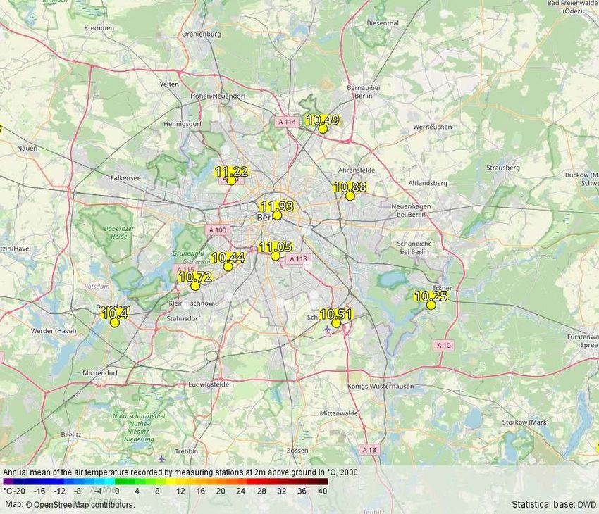
1

Statistical Base
The data used as a statistical base here is part of nationwide data that can be accessed free of charge
on the DWD’s Climate Data Center (CDC) publication platform as the following data set:
Multi-annual means of grids of air temperature (2m) over Germany 1981-2010, Version v1.0.
The grids use the Gauss-Kruger zone 3 coordinate system. The spatial resolution is 1 km x 1 km.
The mean air temperatures are available for different reference periods (1961-1990, 1971-2000, 1981-
2010). They describe the 30-year mean air temperature in 0.1° C increments at 2 m altitude for each
calendar month, the four seasons and the whole year. The winter mean of a year includes the month of
December from the previous year, i.e. the mean winter temperatures for the period 1981-2010 include
December 1980.
The DWD considered potential height dependencies while ascertaining the temperature distributions.
The gridded data does not display processes impacting the climate or weather conditions that are not
directly recorded by the station measuring network or cannot be determined by regression, such as local
effects from an urban heat island outside the observation area of the station network. See DWD 2018
for a complete description of the data set.
The DWD station measurement network covers the entire area of Germany. Its spatial resolution,
however, means that the stations are rather sparsely distributed across the urban area of Berlin,
especially when considering its heterogeneity. The distribution is also not entirely consistent for the
measurement period from 1981 to 2010.
Figure 1 shows the distribution of the available climate stations for the year 2000:

Fig.1: Annual mean of the air temperature recorded by measuring stations at 2m above ground in °C,
for the period of 2000 (DWD Climate Data Center, accessed on February 3, 2021)

2

Methodology
The following steps were taken to evaluate the source grid data of the air temperature (2m) for the
purpose of the Environmental Atlas (cf. Figure 2):
    •   converting and transforming the source data,
    •   increasing the spatial resolution of the temperature distribution by using a suitable interpolation
        procedure, and
    •   deriving a mode of presentation suitable for the map based on isolines and isosurfaces.

Fig. 2: Diagram of how the multi-annual mean grids of air temperature are processed for Berlin, 1981-
2010 (ProAqua using statistical base from DWD 2018)

The source data was available as ASCII grid data in the Gauss-Kruger zone 3 projection. The grids were
converted into the ESRI shape format and then projected into the ETRS1989 UTM 33N coordinate
system that is used in Berlin.
Technically, the data is grid data. According to DWD documentation, however, the temperatures should
be considered point data, which refers to the centre of each grid cell (grid point). The temperature
distribution is a physiographic process. It is continuous and steady. Therefore, the transitions between
the mean temperatures in the individual grid cells should also be smooth. To this end, the source data
(1 km x 1 km resolution) was interpolated to a resolution that is ten times higher, i.e. 100 m x 100 m.
Spatially, the mean temperatures differ only slightly with a range of less than 2°K. They are distributed
relatively homogeneously. The source data is rounded to 0.1°K. This means that the spatial distribution
only contains few distinct value expressions. Due to these constraints, an inverse distance weighted
(IDW) interpolation with a search radius of 16 points was chosen as the interpolation method (cf. ESRI
2019a). The selected method is highly suitable here, as the data is smoothed without the interpolation
fluctuating in the homogeneous value ranges.
Isolines were generated from the interpolated 100 m x 100 m grid data using bilinear interpolation (cf.
ESRI 2019b). Isolines are lines that connect points of equal value. In relation to temperatures, these
lines are also referred to as isotherms, i.e. they connect points of the same temperature. Isosurfaces
3

comprise the areas between two isolines and thus indicate areas with temperatures within a specific
range of values. However, the aforementioned properties of the source data increases the occurrence
of artefacts/ display errors, e.g. along the edges of the grid or where values reach a plateau. The isolines
were therefore adjusted manually afterwards and smoothed using Bézier curves. Subsequently,
isosurfaces were generated from the smoothed isolines.

Map Description
The maps present the mean temperatures for the period from 1981 to 2010 for the entire year and for
the four seasons. The seasons refer to the months as follows:
      •   spring:         March, April, May
      •   summer:         June, July, August
      •   autumn:         September, October, November
      •   winter:         December, January, February
The winter mean of a year includes the month of December from the previous year, i.e. the mean winter
temperatures for the period 1981 – 2010 include December 1980 but do not include December 2010.
The long-term mean air temperatures from 1981 to 2010 range between 9.3°C and 10.4°C (cf. Table 1)
in Berlin, depending on the location. The highest mean temperatures occur in inner city residential areas
between Alexanderplatz and the Görlitzer Park in Kreuzberg. With increasing vegetation and decreasing
building density, the mean temperatures generally decrease successively towards the periphery (Map
04.02.1).
The temperature distributions display very similar characteristics for all five periods analysed (i.e. the
four seasons and the entire year) (cf. Map 04.02.2 through 04.02.5). The influence of the topography is
evident in all periods investigated. In the bottom of Berlin’s glacial valley, which extends from the south-
east to the north-west, the mean temperatures are always a little higher despite the relatively small
difference in altitude (less than 30 m) to the adjacent plateaus.
Table 1 presents a selection of statistical characteristic values for the long-term temperature distribution
from 1981 to 2010 for each period analysed. The analysis refers to the area of Berlin, excluding
surrounding areas.

    Tab. 1: Statistical characteristic values on the long-term mean air temperatures, 1981– 2010
                                  Annual
                                                  Spring         Summer          Autumn          Winter
                                   mean
                         Map      04.02.1         04.02.2         04.02.3        04.02.4         04.02.5
    Minimum [°C]                    9.3              9.1            18.0            9.2            0.7
    Maximum [°C]                    10.4            10.3            19.2           10.4            1.7
    Mean [°C]                       9.72            9.59           18.46           9.67            1.13
    Standard deviation [°C]         0.17            0.17            0.20           0.19            0.16

Tab. 1: Statistical characteristic values on the long-term mean air temperatures, 1981-2010

Previously, the Long-Term Mean Air Temperatures, 1961-1990 were presented based on temperature
time series for different stations. To record the temperature distribution on a small scale, these were
supplemented by a myriad of daytime and nighttime measurement trips on a variety of routes. On the
one hand, the large number of extremely accurate individual measurements was an advantage. On the
other hand, the processing and extensive interpolation of the data, originating from different sources
and recording periods, involved an immense effort.
With their data set “Multi-annual means of grids of air temperature (2m) over Germany 1981-2010”, the
DWD, however, provides extensive and pre-processed information on temperature distributions. This
data forms the basis for the current update of the Environmental Atlas. Due to the different data bases
and resulting differences in methodology, the current results and these of the previous edition of the
Environmental Atlas edition can only be compared to a limited extent.

4

Literature
[1]   DWD (Deutscher Wetterdienst) [Germany’s Meteorological Service] 2018:
      Data set description: Multi-annual means of grids of air temperature (2m) over Germany 1981-
      2010, Deutscher Wetterdienst [Germany’s Meteorological Service] CDC – Vertrieb Klima und
      Umwelt [Climate and Environment Distribution Centre], Offenbach.
      Download PDF (64KB)
      (Accessed on 1 February 2021)
[2]   DWD (Deutscher Wetterdienst) [Germany’s Meteorological Service] 2020:
      Nationaler Klimareport [National Climate Report]. 4th revised edition, Deutscher Wetterdienst
      [Germany’s Meteorological Service], Potsdam.
      Download PDF (9 MB) [only in German]
      (Accessed on 1 February 2021)
[3]   ESRI 2019a:
      ArcGIS Desktop 10.7 Tool reference: How IDW works. Environmental System Research
      Institute, Redlands, CA.
      Internet:
      https://desktop.arcgis.com/en/arcmap/10.7/tools/3d-analyst-toolbox/how-idw-works.htm
      (Accessed on 1 February 2021)
[4]   ESRI 2019b:
      ArcGIS Desktop 10.7 Tool reference: How Contouring works. Environmental System Research
      Institute, Redlands, CA.
      Internet:
      https://desktop.arcgis.com/en/arcmap/10.7/tools/3d-analyst-toolbox/how-contouring-works.htm
      (Accessed on 1 February 2021)
[5]   Stülpnagel, A. 1987:
      Klimatische Veränderungen in Ballungsgebieten unter besonderer Berücksichtigung der
      Ausgleichswirkung von Grünflächen, dargestellt am Beispiel von Berlin-West [Climatic changes
      in conurbations with special emphasis on the compensatory effect of green spaces, illustrated
      by the example of West Berlin], Dissertation at Faculty 14, Technical University of Berlin, Berlin.

Maps:

[6]   SenStadt (Berlin Senate Department for Urban Development) (ed.) 2001:
      Berlin Environmental Atlas, Edition 2001, 04.02 Long-term Mean Air Temperatures 1961-1990,
      1 : 50,000, Berlin.
      Internet:
      https://www.berlin.de/umweltatlas/en/climate/development-of-climate-parameters/1961-
      1990/summary/

5