Machine Learning of polymer types from the spectral signature of Raman spectroscopy microplastics data - arXiv
←
→
Page content transcription
If your browser does not render page correctly, please read the page content below
Machine Learning of polymer types from the
                                          spectral signature of Raman spectroscopy
                                                      microplastics data
arXiv:2201.05445v1 [cs.LG] 14 Jan 2022

                                                                  Sheela Ramanna∗
                                                       Department of Applied Computer Science
                                                               University of Winnipeg,
                                                        Winnipeg, Manitoba R3B 2E9, Canada
                                                             s.ramanna@uwinnipeg.ca
                                                                & Danila Morozovskii
                                                       Department of Applied Computer Science
                                                               University of Winnipeg,
                                                        Winnipeg, Manitoba R3B 2E9, Canada
                                                       morozovskii-d@webmail.uwinnipeg.ca
                                                                  & Sam Swanson
                                                                 Compound Connect
                                                            Winnipeg, Manitoba Canada
                                                           204communications@gmail.com
                                                                 & Jennifer Bruneau
                                                                 Compound Connect
                                                            Winnipeg, Manitoba Canada
                                                             bruneau.jenn@gmail.com
                                                                         January 17, 2022

                                                                               Abstract
                                                The tools and technology that are currently used to analyze chemical
                                            compound structures that identify polymer types in microplastics are not
                                            well-calibrated for environmentally weathered microplastics. Microplastics
                                            that have been degraded by environmental weathering factors can offer
                                            less analytic certainty than samples of microplastics that have not been
                                            exposed to weathering processes. Machine learning tools and techniques
                                            allow us to better calibrate the research tools for certainty in microplastics
                                            analysis. In this paper, we investigate whether the signatures (Raman shift
                                            values) are distinct enough such that well studied machine learning (ML)
                                         ∗ Corresponding   author. This research has been supported by the MITACS Grant IT-18982.

                                                                                    1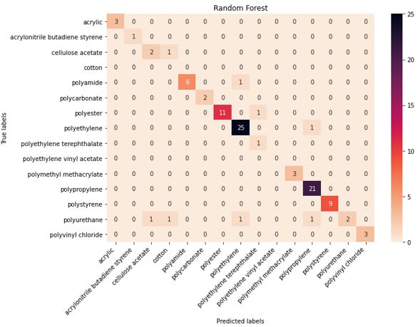
algorithms can learn to identify polymer types using a relatively small
       amount of labeled input data when the samples have not been impacted
       by environmental degradation. Several ML models were trained on a well-
       known repository, Spectral Libraries of Plastic Particles (SLOPP), that
       contain Raman shift and intensity results for a range of plastic particles,
       then tested on environmentally aged plastic particles (SloPP-E) consisting
       of 22 polymer types. After extensive preprocessing and augmentation,
       the trained random forest model was then tested on the SloPP-E dataset
       resulting in an improvement in classification accuracy of 93.81% from 89%.

1      Introduction
Plastic pollution is exclusively the result of anthropogenic activities, with the
majority of plastic entering the environment through land-based activities but
ending up far from their source, having travelled though atmospheric and riverine
pathways and degrading through multiple processes [1]. The durability and
strength of plastics that make them suitable for a broad range of applications
are also what cause them to disperse easily and have led to them becoming
a global pollution problem. The primary reason they pose such a threat to
the environment is their resistance to degradation, allowing them to persist for
hundreds or thousands of years. However, their exposure to a variety of factors
will result in them breaking down from macroplastics to microplastics [2].
    Microplastics are composed of various polymers and include a broad array of
chemical additives [3]. It is understood that microplastics can decay at different
rates depending on climate conditions, and that different stages of decay pose
differing levels of toxicity to plant and animal life [4]. Thus, the chemical diversity
of microplastics is an important consideration. The impacts of microplastics
range from those on marine, freshwater, and terrestrial ecosystems [1], on
human health through ingestion of beverages and contamination in food and
food packaging [5], and on microorganisms through uptake by zooplankton in
freshwater ecosystems or interference with nutrient production and cycling in
aquatic ecosystems. Finally, consumption of microplastics by humans through
the food chain raises concerns about possible health risks and effects on the
human body [2].
    The two most promising techniques for microplastics (less than 5mm) anal-
ysis, are Raman and Fourier transform infrared (FTIR) spectroscopy [6]. The
preferred method for identifying microplastics is Raman spectroscopy which is an
indispensable tool for the analysis of very small microplastics less than 20µm [7].
This is a vibrational spectroscopy technique based on the inelastic scattering
of light [8, 9]. When laser light is shone on a plastic particle, a small amount
of this light shifts in energy from the laser frequency because of interactions
between the incident electromagnetic waves and the vibrational energy levels of
the sample’s molecules. A Raman spectrum of the sample is created by plotting
the Raman shift against the light frequency1 . For example, in Fig 1, the y-axis
    1 https://www.utsc.utoronto.ca/~traceslab/PDFs/raman_understanding.pdf

                                           2
gives the intensity of the scattered light, and the x-axis gives the energy of light.
The specific type of material is marked with peaks in Raman spectroscopy. One
of the primary advantages of Raman spectroscopy is that even after exposure to
ultraviolet (UV) light, the Raman spectra of microplastics are not significantly
altered; this is significant as microplastics typically experience multiple forms of
degradation with the majority of microplastics samples being degraded [10].
    Machine learning (ML) algorithms such as Decision Trees (DT), Random
Forest (RF), Support Vector Machines (SVM), K-Neighbour methods (KNN),
Artificial Neural Networks (ANN) have been successfully applied to Raman
spectra data in diverse areas of science. In [11], ANN and KNN methods were
used to predict the concentration of cocaine using Raman spectroscopy. The
authors [12], use Raman spectroscopy to detect chemical changes in melanoma
tissue of patients and achieve 85% (sensitivity) and 99% (specificity) results with
ANNs. In [13], several well-known ML algorithms were applied to determine
the mine of origin and extraction depth of samples by finding Raman spectral
differences for variscite (phosphate mineral) specimens from the Gavà mining
complex where the SVM classifier gave the best result of almost 90% classification
accuracy. In [14], the SVM model was able to achieve a diagnostic accuracy of
92% for tuberculosis patients using Raman spectra of blood sera. RF classifier
was used in the analysis of spectral information of various cultural heritage
materials by [15]. The authors [16], classify seven types of oils using Raman
spectroscopy: sunflower, sesame, hemp, walnut, linseed (flaxseed), sea buckthorn
and pumpkin seeds where a subspace KNN ensemble classifier gave the best
classification accuracy of 88.9%. In [17], the authors explore association between
Raman spectroscopy and machine learning to differentiate fruit distillate samples
(alcoholic beverage) to determine trademark, geographical and botanical origin.
The best geographical classification of the fruit distillates was obtained with
the ensemble (subspace KNN) method resulting in an accuracy of 90.9% for 30
samples. In [18], ANN and SVM algorithms were used to diagnose biochemical
composition of biological fluids of patients with Alzheimer’s disease based on
near infrared (NIR) Raman spectroscopy with 84% sensitivity and specificity
values. The authors [19], present deep learning methods to extract and analyze
chemical information in big and complex datasets derived from Raman and
surface-enhanced Raman scattering (SERS) techniques. In [20], 230 Raman
spectra samples of high dimensional solvent and solvent mixtures (chemicals)
were classified with deep neural networks using a locally connected architecture,
resulting in a mean accuracy of 96.0%. In [21], Raman spectra of oral tongue
squamous cell carcinoma and para-carcinoma tissues of 24 patients were analyzed.
A convolutional neural network model was used to extract features, which were
then input to an SVM classifier resulting in a 99.96% accuracy. AlexNet deep
learning model was used to classify chronic renal failure using serum Raman
spectra of 100 patients with an accuracy of 95.22% [22].
    In [23], six types of common household plastics using Raman spectroscopy
were evaluated to demonstrate the potential of machine learning methods such
as principle component analysis, KNN as well regression models for classification
and prediction. In [24], hyperspectral imaging was used to detect micro plastic

                                         3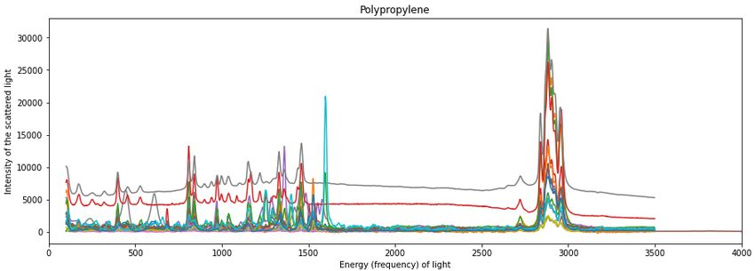
contamination in soils. Classification precision of 86% for polymers containining
microplastics particles of size between 1-5 mm and about 99% precision for
microplastics particles of size between 0.5-1 mm were obtained. In [25] laser-
induced breakdown spectroscopy was used to create plastic samples containing
different additives such as flame retardants. Principle component analysis (PCA)
and Linear Discriminant Analysis (LDA) were used to discriminate 11 different
types of additives with LDA achieving almost 100% accuracy. In [26], 4000
images belonging to the five categories of plastic resin codes from a public
database were classified using convolutional neural networks with an accuracy
of 99.79%. In [27], micro Fourier Transform Infrared (µ-FTIR) hyper-spectral
imaging with Partial least squares discriminant analysis (PLS-DA) and soft
independent modelling of class analogy (SIMCA) which is based on PCA, were
used to classify nine of the most common polymers in microplastics found on
seabed sediment samples. A review of polymer informatics is presented in [28].
In [29], PCA and clustering with K-means on short wave infrared hyperspectral
data prepared using reflection imaging with a hyperspectral camera was used to
analyze and classify 13 commercially available plastics.
    Our work differs from the more recent work where either hyperspectral
imaging, digital images or laser-induced breakdown spectroscopy of plastics
were used with machine learning models including deep learning models. The
datasets used were either prepared by the authors or included large image
repositories suitable for deep learning. On the other hand, Raman spectroscopy
data typically consist of approximately 1,000 to 3,000 data points. It is difficult
and expensive to obtain the spectroscopy data, and only a limited amount of
data is available online. Additionally, each sample might contain not one type
of microplastic, but rather a combination of materials. To this end, in our
work, several machine learning models were trained on a well-known repository,
Spectral Libraries of Plastic Particles (SLOPP) containing 148 samples and
158 samples from Mendeley 2 . The SLOPP library contains Raman shift and
intensity results of Raman spectroscopy laboratory analyses conducted at the
Rochman Lab 3 in the Department of Ecology and Evolutionary Biology at the
University of Toronto for a range of plastic particles. This library also includes
environmentally aged plastic particles (SloPP-E) containing 97 samples. After
extensive preprocessing and augmentation, the trained random forest model was
then tested on the SloPP-E dataset resulting in an improvement in classification
accuracy of 93.81% from 89%. This work contributes to the understanding
of environmental polymers by validating the machine learning methods that
improve the predictive capability of Raman spectroscopy data analysis.
    Our paper is organized as follows: In section 2, we give a description of the
open source spectroscopy datasets considered in this work. In section 3, we
present a detailed discussion of the preprocessing and augmentation techniques
used in this research for generating training and testing examples. In section 4,
we give an in-depth analysis of the classification results of our final model followed
  2 https://data.mendeley.com/datasets/kpygrf9fg6/1
  3 https://rochmanlab.wordpress.com/spectral-libraries-for-microplastics-research/

                                            4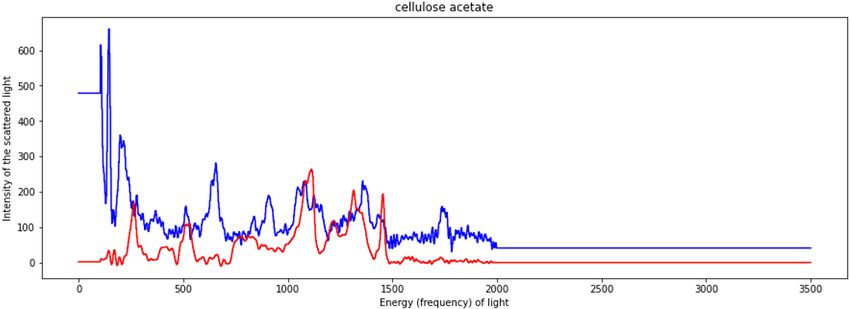
by concluding remarks in section 5.
2 MATERIALS- SPECTROSCOPY DATA
A Raman spectrum can provide molecular bond information on a particular
substance and may be described as a “fingerprint” of the substance due to its
uniqueness [30]. Raman spectra are a plot of scattered intensity as a function
of the energy difference between the incident and scattered photons and are
obtained by pointing a monochromatic laser beam at a sample [31]. The resultant
spectra are characterized by shifts in wave numbers (inverse of wavelength in
cm− 1 ) from the incident frequency. The frequency difference between incident
and Raman-scattered light is termed the Raman shift, which is unique for
individual molecules. For this research, the following datasets have been used
SLoPP, SLoPP-E, Mendeley. A combined dataset of SLoPP and Mendeley was
used as our training dataset, while SLoPP-E was used as the testing dataset.
SLOPP: SLoPP is a spectral library of microplastic particles with 148 samples,
having different polymer types (shown in Table 1), colours and morphologies.
Examples of colours are turqoise, orange, green, white, grey, black, light
brown and clear. Examples of morphologies include: fragments, sphere,
film, foam, and fiber. SLoPP was collected in the range of 100-3500 cm− 1
and was created to include commonly used plastics.
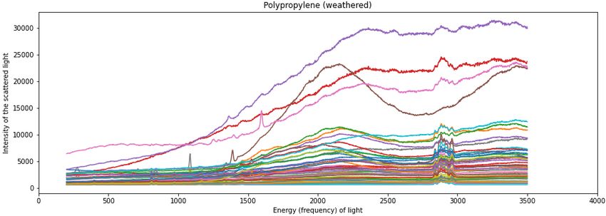
Fig. 1 illustrates the Raman spectra for one type of polymer (polypropylene).
The y-axis shows the intensity of the scattered light, and the x-axis shows
the energy (frequency) of light. Different colours represent different samples
in the dataset. It can be observed, that the most distinguishing feature of
the Raman spectroscopy is spikes on different energies of the light.
Figure 1: Raman spectra of Polypropylene from the SLoPP dataset.
SLOPP-E: SLoPP-E dataset is similar to the SLoPP dataset, however, it
includes samples exposed to a variety of environmental conditions (e.g.,
some samples have undergone some chemical degradation, ageing). The
5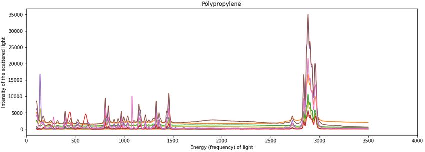
microplastics in this library SLoPP-E include environmental samples ob-
     tained across a range of matrices, geographies, and time. Fig. 2 llustrates
     the Raman spectra for the same type of polymer (polypropylene) as the
     one shown in Fig. 1. Different colours represent different samples in the
     dataset. It can be observed that these two datasets share the same values
     on the x-axis (frequency) and similar intensities (spikes on the y-axis) for
     the same polymer type.

    Figure 2: Raman spectra of Polypropylene from the SLoPP-E dataset.

    Table 1 shows the distribution of polymers types for SLoPP and SLoPP-E.
It can seen that some types are either missing in training (SLoPP) or testing
(SLoPP-E) datasets. However, the training dataset includes many more types
that are missing compared to the testing dataset.

 Mendeley: This dataset has two variations of microplastics: standard and
    weathered. The standard data is similar to SLoPP and the weathered
    data is similar to SLoPP-E (by description), subjected to environmental
    conditions.

    Figure 3: Raman spectra of Polypropylene from the Mendeley dataset.

                                       6
Polymer Types SLoPP samples SLoPP-E samples
Acrylic 10 3
Acrylonitrile Butadiene Styrene 10 1
Cellulose Acetate 4 3
Cotton 16 -
Polyamide 7 7
Polycarbonate 7 2
Polyester 10 12
Polyethylene 24 26
Polyethylene Terephthalate 9 1
Polyethylene Vinyl Acetate 5 -
Polymethyl Methacrylate 1 3
Polypropylene 17 21
Polystyrene 11 9
Polyurethane 6 6
Polyvinyl Chloride 11 3
Dyed Cellulose - 5
Polybutylene Terephthalate - 1
Polyethylene Terephthalate-co-Polycarbonate - 1
Polyethylene-co-Polypropylene - 3
Polystyrene-co-Polyvinyl Chloride - 1
Polysulfone - 1
Rubber - 4
Table 1: Data Distribution for SLoPP and SLoPP-E.
A plot of the Raman spectroscopy for polypropylene is shown in Fig. 3.
From this plot, one can observe the following : i) some samples in the
Mendeley dataset have a wave-like structure, and ii) the peaks (intensities
of scattered light) are not as sharp and separated as in the SLoPP or
SLoPP-E datasets. Table 2 shows the data distribution for Mendeley
dataset. The majority of samples in this dataset belong to two polymer
types: polypropylene and polyethylene and can be used in the training
dataset, as they are also present in the SLoPP dataset.
2.1 Final dataset
The final dataset used in our experiments is shown in Table 3. Note, that only
the polymer types that are present in SLoPP are used. The majority of samples
come from SLoPP, however, Mendeley contains a lot of samples for the polyester,
polyethylene and polypropylene polymer types. The test dataset consists of
only SLoPP-E, which was reduced to match the classes (SLOPP polymer types)
present in the training set. 16 samples from 7 different types of plastic have
7Polymer Types Mendeley samples
Not detected 8
Acrylonitrile Butadiene Styrene 1
Nitrocellulose 1
Polyamine (nylon) 6
Polycarbonate 2
Polyethylene 74
Polyester 16
Polypropylene 54
Polystyrene (maybe) 2
Polyvinyl chloride 9
Table 2: Data Distribution for Mendeley.
been removed resulting in a combined dataset of 306 training samples and 97
testing samples.
Polymer Types SLoPP SLoPP-E Mendeley
Acrylic 10 3 -
Acrylonitrile Butadiene Styrene 10 1 1
Cellulose Acetate 4 3 -
Cotton 16 - -
Polyamide 7 7 -
Polycarbonate 7 2 2
Polyester 10 12 16
Polyethylene 24 26 74
Polyethylene Terephthalate 9 1 -
Polyethylene Vinyl Acetate 5 - -
Polymethyl Methacrylate 1 3 -
Polypropylene 17 21 54
Polystyrene 11 9 2
Polyurethane 6 6 -
Polyvinyl Chloride 11 3 9
Table 3: Final dataset (SLoPP, SLoPP-E, Mendeley).
3 METHODS: FEATURE ENGINEERING AND
PREPROCESSING
As has been discussed in the previous section, different polymer types can be
identified by the location of spikes on the x-axis (energy). Before this data
can be used for classification learning, feature engineering which includes data
8transformation as well as preprocessing techniques such as normalization and
discretization have been used. These techniques are described below.
3.1 Normalization
Here we discuss scaling methods for normalizing both the intensity (y-axis) and
energy (x-axis) feature values since there are multiple problems with the feature
values such as: varying ranges, varying step values, integer vs. real values as
well negative values. Alg. 1 gives the pseudo-code for scaling the energy values.
• Energy values: Each sample in the dataset has a different x-axis range
(i.e., one sample might have y-axis values between 100 and 1200 on the
x-axis and another one between 300 and 3000). Furthermore, each sample’s
range between individual points on the x-axis is different as well (i.e., one
sample can have a step value of 2 and another sample with a step value of
3). Therefore, scaling of the x-axis should be performed, where all values
would be mapped to the corresponding points. Additionally, x-axis values
are continuous values (ex: real value of 101.23), therefore, x-axis values
should be mapped to integer values.
Scaling works as follows: firstly, as each sample has a different x-axis
range, these values are mapped to the same range, by finding the minimum
and maximum value of x for all samples (shown as parameter min_range,
max_range in Alg. 1). In the case of the combined dataset, these parameter
values are set to 0 and 3500 respectively. Then the values are populated by
either the first value if the values occur at the beginning of the dataset, or
by the last value if the values occur at the end. For example, if a sample
has values on the x-axis ranging between 100 and 3000, then the values
between 0-99 are populated with 100, and the values between 3001-3500
are populated with the value 3000.
Secondly, as samples have a different step between each value, the gaps
between these values are populated with the value which is at the beginning
of a gap (i.e., if the x-values of two samples are 100 and 103, then all
x-values having either 101 and 102 are replaced with value 100). As a result,
this function produces 3501 points (3500 - 0 + 1), which are populated
using the information from the original sample.
• Intensity values: Some samples in the SLoPP-E test set have negative
values for the intensity (y-axis). Hence, all values have been scaled by
adding a constant factor of one unit, which is the minimum negative value
on the y-axis plus 1. This also ensures that there are no zero values.
3.2 Data Transformation
Two well-known data transformation techniques were used: Rate of Change
(ROC) and Percentage Change (PC) shown in Eqns. 1 and 2. Both these
9Algorithm 1 Scaling(Dataset, min_range, max_range)
1: dataset_scaled ← dict()
2: for plastic_type, idxs in Dataset.items() do
3: dataset_scaled[plastic_type] ← []
4: for idx in idxs do
5: changed_data ← DataF rame({0 x0 :
0 0
range(min_range, max_range + 1), y : [0.0] ∗ (max_range + 1)})
6: last_element_idx ← −1
7: for index, point in idx.iterrows() do
8: idx_of _el ← int(point[0 x0 ])
9: if idx_of _el > max_range then
10: break
11: if last_element_idx != −1 then
12: for i in range(last_element_idx + 1, idx_of _el) do
0 0
13: changed_data.at[i, y] ←
0 0
changed_data.at[last_element_idx, y ]
14: else
15: for i in range(idx_of _el) do
16: changed_data.at[i, 0 y 0 ] ← point[0 y 0 ]
17: changed_data.at[idx_of _el, 0 y 0 ] ← point[0 y 0 ]
18: last_element_idx ← idx_of _el
19: for i in range(last_element_idx + 1, max_range + 1) do
20: changed_data.at[i, 0 y 0 ] ← changed_data.at[last_element_idx,
0 0
y]
21: dataset_scaled[plastic_type] ← dataset_scaled[plastic_type] +
changed_data
22: return dataset_scaled
10techniques modify the original data by making sharp changes in the original
dataset more visible.
• Rate of Change (ROC):
f (b) − f (a)
ROC = (1)
b−a
where f(a) and f(b) are values on the y-axis and a and b are their corresponding
values on the x-axis.
• Percentage Change (PC):
f (a)
PC = (2)
mean(f (a − 1), ...., f (a − n))
where f(a) is the current value of the intensity (y-axis) and n is the number of
values on the y-axis.
Figure 4: Sample for polymethyl methacrylate.
Figure 5: ROC processed sample for polymethyl methacrylate.
11Since the PC function did not give good classification results, the ROC
function was used as the main data transformation technique. However, the PC
function was used in the augmentation of the training set, which is described later
in Sec. 3.4. As an illustration of this technique, we present two figures. Fig. 4
shows the plot for a single sample of type polymethyl methacrylate. Fig. 5 shows
the transformed plot. The ROC transformation was applied to the intensity
values (y-axis) which results in sharp spikes and preserves the changes in intensity
values at the same energy (x-axis) co-ordinate. It should be noted that, the
values on the y-axis can be either positive or negative, meaning a positive or
negative rate of change.
3.3 Discretization- smoothing by bin-means
Since Raman spectroscopy data has the characteristics of time-series data, the
spikes in the distribution are the most important patterns that can be extracted
from the samples. An equal-width binning technique was used in this research.
Then a smoothing by bin-means technique is applied where the average of the
values in a bin is calculated and each bin is now represented using the average
value. Fig. 6 shows the results of this technique applied to a single sample for
polymethyl methacrylate type with a bin width of 11. That is, every 11 values
are mapped to the same bin, and the average value of the bin is calculated. One
can also observe the compressed scale on the x-axis as compared to the scale in
Fig. 5.
Figure 6: Binning technique of ROC processed sample for polymethyl methacry-
late.
3.4 Augmentation
As the dataset is very small, the data augmentation function has been imple-
mented to populate the training dataset with more samples. The pseudo-code
for the augmentation process is given in Algorithms 3-5.
The augmentation function works the following way: firstly, the function
iterates over a polymer (plastic) type that needs to be augmented, and the
12pct_change function is used to calculate the change between the current and
the previous value of a sample, by dividing the two numbers. This helps to keep
information about the changing values.
Secondly, a random uniform distribution is applied, where random values be-
tween -0.05 and 0.05 are chosen. This is a user-defined parameter random_change
and controls how much the augmented dataset differs from the original sample.
The last step is to reverse the percentage change function, by multiplying
the original value with the new percentage change value. As the percentage
change value has been changed slightly, each generated value is different from the
original value. However, such a change leads to a problem of rapidly increasing
or decreasing graph fluctuations. These sharp fluctuations are controlled by the
max_pct_change parameter. This parameter value is set to 99, meaning that
the generated value could be up to 99% more than the original value or 99%
less than the original value. Additionally, Alg. 3 includes parameter shift. This
parameter is meant to shift the values on the y-axis (higher or lower). However,
this value was set to 0, as it does not change the test accuracy significantly.
Algorithm 2 Generate_Augmented_Data(train_dataset, plastic_type_list,
min_num_examples, random_change=0.05, shift=0, max_pct_change=99)
1: plastic_type_list ← [el.lower() for el in plastic_type_list]
2: train_dataset_augm ← train_dataset
3: for plastic_type, idxs in train_dataset.items() do
4: iterate ← 0
5: if plastic_type in plastic_type_list then
6: while len(train_dataset_augm[plastic_type]) <
min_num_examples do
7: cur_idx ← iterate % len(idxs)
8: pct_change_list ← pct_change(idx[cur_idx][0 y 0 ])
9: augm_example ← get_augmented_example(pct_change_list, random_change)
10: init_value ← idxs[cur_idx][0 y 0 ][0]
11: if min(idxs[cur_idx][0 y 0 ]) ≤ 0 then
12: init_value ← init_value + abs(min(idxs[cur_idx][0 y 0 ])) + 1
13: augmented_data ← get_f ull_augmented_example(idxs[cur_idx][0 y 0 ],
augm_example, init_value, shif t, max_pct_change)
14: train_dataset_augm[plastic_type] ←
train_dataset_augm[plastic_type] + DataF rame({0 x0 :
idxs[cur_idx][0 x0 ], 0 y 0 : augmented_data})
15: iterate ← iterate + 1
16: train_dataset ← train_dataset_augm
Example of augmented data is shown in Fig. 7. The line which is coloured
red is the original sample, and a blue line is the augmented sample. It can
be seen, that the augmented sample keeps the same trajectory as the original
sample, but introduces some changes on the y-axis values. Spikes on generated
samples are retained on same x-axis values, however, the intensity of such spikes
13Algorithm 3 pct_change(dataframe)
1: pct_change_list ← []
2: min_value ← min(dataf rame)
3: if min_value ≤ 0 then
4: dataf rame ← [i + abs(min_value) + 1 for i in dataf rame]
5: for num, _ in enumerate(dataf rame[:len(dataf rame) − 1]) do
6: pct_change_list ← pct_change_list + (dataf rame[num +
1]/dataf rame[num])
7: return pct_change_list
Algorithm 4 get_augmented_example(pct_change_list, ran-
dom_change=0.2)
1: augm_pct_change_list ← []
2: for el in pct_change_list do
3: tmp_el ← el + random.unif orm(−random_change, random_change)
4: if tmp_el ≤ 0 then
5: tmp_el ← el . el is > 0, because of pct_change function
6: augm_pct_change_list ← augm_pct_change_list + tmp_el
7: return augm_pct_change_list
Algorithm 5 get_full_augmented_example(original_dataset,
pct_change_list, init, shift=0, max_pct_change=10)
1: previous_value ← init + shif t
2: augm_pct_change_list ← []
3: augm_pct_change_list ← augm_pct_change_list + previous_value
4: min_value ← min(original_dataset)
5: if min_value ≤ 0 then
6: original_dataset ← [i + abs(min_value) + 1 for i in original_dataset]
7: for num, el in enumerate(pct_change_list) do
8: previous_value ← previous_value ∗ el
9: if previous_value > original_dataset[num + 1] ∗ (1 +
max_pct_change/100) then
10: previous_value ← original_dataset[num + 1] ∗ (1 +
max_pct_change/100)
11: if previous_value < original_dataset[num + 1] ∗ (1 −
max_pct_change/100) then
12: previous_value ← original_dataset[num + 1] ∗ (1 −
max_pct_change/100)
13: augm_pct_change_list ← augm_pct_change_list + previous_value
14: return augm_pct_change_list
14is different.
Figure 7: Improved augmented data (red – original; blue – augmented).
In our research, we have augmented polymer types that have either a small
number of samples (e.g., less than 5) or have performed poorly on test results.
4 RESULTS AND DISCUSSION
In this section, we analyze the results of the experiments. The following ML
algorithms have been used in this research using the scikit-learn workbench4 :
support vector machines (SVM), random forest (RF), decision tree (DT), k-
nearest neighbours (KNN), and artificial neural network (ANN). The RF model
is the only model that gives high classification accuracy. Hence, in our discussions
related to the analysis of the effect of different preprocessing, discretization as
well as augmentation techniques, we will use the RF model as our baseline model.
In an effort to increase the training set size, we also experimented with another
microplastic dataset Open Specy 5 . This dataset contains a total of 183 examples
and 137 polymer types [32]. We observed that most of the polymer types in this
dataset do not appear in SLoPP, therefore, cannot be used. Additionally, the
intensities of the scattered light (y-axis) for Open Spacy dataset is normalized to
values between 0 and 1, and there the original values for the intensities cannot be
reconstructed. As a result, this dataset was not used in our final model training
experiments.
Table 4 presents experiments using different preprocessing functions and
with no scaling of the y-axis values. All experiments were conducted with
a combination of the scaling and ROC transformation methods described in
sections 3.1 and 3.2. The best result (accuracy of 79.38% highlighted in blue)
4 https://scikit-learn.org/stable/
5 https://doi.org/10.1021/acs.analchem.1c00123.s001
15Experiment Preprocessing Methods RF Accuracy (%)
1 scaling (x-axis), ROC 79.38
2 scaling (x-axis), no ROC 61.85
3 no scaling (x-axis), ROC 72.16
4 no scaling(x-axis), no ROC 53.61
Table 4: Model accuracy with different variations of preprocessing functions.
was achieved with scaling energy values and using the rate of change transformed
feature.
Fig. 8 shows the performance of the RF model using different bin sizes
ranging from 2 to 50. The discretization technique which achieves the best result
(classification accuracy 86.59% with information gain criteria) is when the bin
size is between 10 and 20. This experiment does not use any augmentation
method.
Figure 8: Accuracy of the model with different bin sizes.
However, if the training dataset is augmented, the accuracy increases dra-
matically (see Fig. 9). Augmentation has been applied to the following polymer
types: Cellulose Acetate, Polyamide, Polymethyl Methacrylate and Polyurethane,
where each type has been augmented up to 15 examples. Experiments were
conducted with two different criteria for the RF model, information gain (in
Fig. 9) and gini (in Fig. 10). One can observe that the classification accuracy is
not as good with the gini criteria as with the information gain criteria.
The best result of 91.75% classification accuracy was obtained with a bin
size of 12 and information gain (entropy) as the criteria for tree construction.
Fig. 11 gives the confusion matrix with classification details for each polymer
type in the SLOPP-E dataset. It can be seen, that the model detects most of
the samples correctly. However, it misclassifies a few samples, especially the
Polyurethane polymer where 4 out of 6 samples were misclassified. The training
accuracy of this model is 100%, which signifies that the model overfits. This is
due to the fact that that the model was trained on just 306 samples.
Table 5 shows the most commonly occurring misclassified samples. The
16Figure 9: Accuracy of the model with different bin size with augmented data
with information gain criteria.
Figure 10: Accuracy of the model with different bin size with augmented data
with gini criteria.
model always predicts the same polymer type for these samples, irrespective
of how the data has been processed. Upon examination of the corresponding
Raman spectroscopy plots, it is hard to detect whether the sample is mislabeled
or the model predicts the result wrongly (Fig. 12-13). Fig. 12 shows a sample of
a type cellulose acetate, plotted with one example from a train dataset of cotton
type (incorrect type). The spike around 1000 value on the x-axis has the same
shape as other spikes which do not fully correspond to this type (cotton). Fig.
13 shows a sample of cellulose acetate type, plotted with one example from a
train dataset of the same type (correct type). It can be observed, that these
samples have a different shape compared to the one in Fig. 12. Hence these
samples do not match.
Since the SLoPP-E test set was subject to weather and ageing, another
experiment was conducted by adding some noise to the training (SLoPP) dataset
to introduce some non-linearity. For each value on the x-axis, a small random
17Figure 11: Confusion matrix for the model that achieved 91.75% accuracy.
Sample number Model predicted Actual label
6 Cotton Cellulose Acetate
12 Polyethylene Polyamide
24 Polyethylene Terephthalate Polyester
50 Polyurethane Polyethylene
88 Cellulose Acetate Polyurethane
89 Polyamide Polyurethane
Table 5: Misclassified cases.
value was either added or subtracted. However, the addition of noise did not
change the accuracy in any significant way (see Fig. 14).
The final model was trained on augmented data, which was preprocessed using
the following functions: ROC, scaling x-axis (0-3500), discretization with the
window size 12, no y-axis rescaling. The following polymer types were augmented:
Cellulose Acetate, Polyamide and Polyurethane (30 samples), Polyester (40
samples), Polymethyl Methacrylate (10 samples) and Polystyrene (20 samples).
Figure 15 gives the confusion matrix where the trained model detects most
of the samples correctly, and only a few samples are mislabeled. The model
mostly performs poorly on the Polyurethane type, as it misclassifies 3 out of 6
18Figure 12: Wrongly detected sample (red) plotted on a wrongly predicted type
(blue).
Figure 13: Wrongly detected sample (red) plotted on a correct type (blue).
Figure 14: Accuracy of the model with noise added to the training dataset.
test samples. The Acrylonitrile Butadiene Styrene type also performs poorly, as
it misclassifies a single test sample. Since there is only 1 test sample available,
this classification could be misleading.
19Figure 15: Confusion matrix for the model that achieved 93.81% accuracy.
Table 6 gives the results of experiments with other models. However, none
of the other models achiev the same accuracy on the test dataset as the random
forest model. The ANN model with 4 layers of 128, 64, 32 and sparse categorical
cross-entropy was used with the adam optimizer. SVM with linear kernel (it
produced the best accuracy, compared to other kernels), DT (with entropy) and
KNN with 3 nearest neighbours were used.
Models Classification Accuracy
ANN 71.13%
SVM (linear kernel) 73.19%
DT 69.07%
KNN 73.19%
Table 6: Accuracies of different machine learning models.
In summary, our experiments demonstrate that there is a significant improve-
ment in the classification accuracy (from 89% to 93.81%) when the dataset is
augmented. This shows that a larger data set with more training and balanced
20samples can improve the classification performance beyond 94% and learn from
environmentally degraded samples. The other important issue is that there
is some concern that the original sample maybe mislabeled. This is because
the predicted type (by the model) is not similar to the actual type (visually).
Another observation is that even when wave-like samples (from the Mendeley
dataset) were excluded from the training set, the classification accuracy was
around 90%. This shows that adding the samples (even though some of the
shapes were different) may have in fact helped the model to learn, or at least,
did not have a negative effect on the model. One reason could be that SLoPP-E
(test dataset) does not have similar wave-like samples.
5 Conclusion
In this work, we were primarily interested in detecting polymer types from
the spectral signature of Raman spectroscopy microplastics data which were
environmentally aged from a well-known dataset. Environmental weathering
occurs from exposure to temperature extremes, UV radiation, wind, water ero-
sion in freshwater environments, and saltwater erosion in marine environments,
in addition to other factors in localized ecosystem contexts. Exposure of mi-
croplastics to the environment affects their spectrographic output data, making
spectrographic analysis results less reliable than unaffected samples. Different
normalization methods as well as data transformation methods for preprocessing
and feature engineering were applied. Since the number of training samples
in certain polymer types were limited, a data augmentation method was used.
Different ML models were trained with the random forest model giving the best
result with an improvement in classification accuracy of 93.81% from 89%. A
detailed discussion of the results is presented in an effort to contribute to the
understanding chemical compounds of plastics that have been weathered by
various environmental processes. The significance of this research project is to
strive for a measurably improved predictive capacity of Raman spectroscopy
data to help classify polymer types through an applied machine learning process.
This work can lead to applications in ecotoxicology and environmental research,
the circular economy for plastics recycling processes, water quality testing and
treatment processes, food and beverage quality control testing, to name a few.
References
[1] A. Booth, L. Sørensen, Microplastic fate and impacts in the environment,
in: C. M. T. Rocha-Santos, M. Costa (Ed.), Handbook of Microplastics in
the Environment, Springer International Publishing, Cham, 2020, pp. 1–24.
URL https://doi.org/10.1007/978-3-030-10618-8_29-1
[2] J. Conesa, M. Iñiguez, Analysis of microplastics in food samples, in: C. M.
T. Rocha-Santos, M. Costa (Ed.), Handbook of Microplastics in the Envi-
21ronment, Springer International Publishing, Cham, 2020, pp. 1–16.
URL https://doi.org/10.1007/978-3-030-10618-8_5-1
[3] C. M. Rochman, C. Brookson, J. Bikker, N. Djuric, A. Earn, K. Bucci,
S. Athey, A. Huntington, H. McIlwraith, K. Munno, H. De Frond, A. Kolomi-
jeca, L. Erdle, J. Grbic, M. Bayoumi, S. Borrelle, T. Wu, S. Santoro, L. Wer-
bowski, X. Zhu, R. Giles, B. Hamilton, C. Thaysen, A. Kaura, N. Klasios,
L. Ead, J. Kim, C. Sherlock, A. Ho, C. Hung, Rethinking microplastics
as a diverse contaminant suite, Vol. 38, Environmental Toxicology and
Chemistry, 2019, pp. 703–711.
URL https://doi.org/10.1002/etc.4371
[4] S. Pflugmacher, J. H. Huttunen, M.-A. von Wolff, O.-P. Penttinen, Y. J.
Kim, S. Kim, S. M. Mitrovic, M. Esterhuizen-Londt, Enchytraeus crypticus
avoid soil spiked with microplastic, Canadian Journal of Fisheries and
Aquatic Sciences 8 (1).
URL https://doi.org/10.3390/toxics8010010
[5] E. Fournier, L. Etienne-Mesmin, S. Blanquet-Diot, M. Mercier-Bonin, Im-
pact of microplastics in human health, in: C. M. T. Rocha-Santos, M. Costa
(Ed.), Handbook of Microplastics in the Environment, Springer International
Publishing, Cham, 2021, pp. 1–25.
URL https://doi.org/10.1007/978-3-030-10618-8_48-1
[6] L. Cabernard, L. Roscher, C. Lorenz, G. Gerdts, S. Primpke, Comparison
of raman and fourier transform infrared spectroscopy for the quantification
of microplastics in the aquatic environment, Environ. Sci. Technol. 52 (22)
(2018) 13279––13288.
URL https://doi.org/10.1021/acs.est.8b03438
[7] C. F. Araujo, M. M. Nolasco, A. M. Ribeiro, P. J. Ribeiro-Claro, Identifica-
tion of microplastics using raman spectroscopy: Latest developments and
future prospects, Vol. 142, Water Research, 2018, pp. 426–440.
URL https://doi.org/10.1016/j.watres.2018.05.060
[8] X. Zhu, B. Nguyen, J. B. You, E. Karakolis, D. Sinton, C. Rochman,
Identification of microfibers in the environment using multiple lines of
evidence, Vol. 53, Environmental Science and Technology, 2019, pp. 11877–
11887.
URL https://doi.org/10.1021/acs.est.9b05262
[9] M. N. Popov, J. Spitaler, V. K. Veerapandiyan, E. Bousquet, J. Hlinka,
M. Deluca, Raman spectra of fine-grained materials from first principles,
Vol. 6, npj Computational Materials, 2020.
URL https://doi.org/10.1038/s41524-020-00395-3
[10] M. Liu, S. Lu, Y. Chen, C. Cao, M. Bigalke, D. He, Analytical methods
for microplastics in environments: Current advances and challenges, in:
v. D. He, M. Costa (Ed.), The Handbook of Environmental Chemistry:
22Microplastics in Terrestrial Environment, vol. 95, Springer International
Publishing, Cham, 2020, pp. 3–24.
[11] M. G. Madden, A. G. Ryder, Machine learning methods for quantitative
analysis of raman spectroscopy data, Vol. 4876, Proceedings of SPIE - The
International Society for Optical Engineering, 2002.
URL https://doi.org/10.1117/12.464039
[12] M. Gniadecka, P. A. Philipsen, S. Wessel, R. Gniadecki, H. C. Wulf, S. Sig-
urdsson, O. F. Nielsen, D. H. Christensen, J. Hercogova, K. Rossen, H. K.
Thomsen, L. K. Hansen, Melanoma, Diagnosis by raman spectroscopy and
neural networks: Structure alterations in proteins and lipids in intact cancer
tissue, Journal of Investigative Dermatology 122 (2004) 443–449.
[13] J. Diez-Pastor, S. Jorge-Villar, A. Arnaiz-Gonzalez, C. Garcia-Osorio,
Y. Diaz-Acha, M. Campeny, J. Bosch, J. Melgarejo, Machine learning
algorithms applied to raman spectra for the identification of variscite origi-
nating from the mining complex of gava, Raman Spectroscopy (2018) 1––12.
URL https://doi.org/10.1002/jrs.5509
[14] S. Khan, R. Ullah, S. Shahzad, N. Anbreen, M. Bilal, A. Khan, Anal-
ysis of tuberculosis disease through raman spectroscopy and machine
learning, Photodiagnosis and Photodynamic Therapy 24 (2018) 286–291.
doi:https://doi.org/10.1016/j.pdpdt.2018.10.014.
URL https://www.sciencedirect.com/science/article/pii/
S1572100018302539
[15] V. Sevetlidis, G. Pavlidis, Effective raman spectra identification with
tree-based methods, Journal of Cultural Heritage 37 (2019) 121–128.
doi:https://doi.org/10.1016/j.culher.2018.10.016.
URL https://www.sciencedirect.com/science/article/pii/
S1296207418303595
[16] C. Berghian-Grosan, D. Magdas, Raman spectroscopy and machine-learning
for edible oils evaluation, Vol. 218, 121176, Talanta, 2020.
URL https://doi.org/10.1016/j.talanta.2020.121176
[17] C. Berghian-Grosan, D. Magdas, Application of raman spectroscopy and
machine learning algorithms for fruit distillates discrimination, Vol. 10,
21152, Scientific Reports, 2020, pp. 3320–3328.
URL https://doi.org/10.1038/s41598-020-78159-8
[18] E. Ryzhikova, N. M. Ralbovsky, V. Sikirzhytski, O. Kazakov, L. Halamkova,
J. Quinn, E. A. Zimmerman, I. K. Lednev, Raman spectroscopy and
machine learning for biomedical applications: Alzheimer’s disease diag-
nosis based on the analysis of cerebrospinal fluid, Spectrochimica Acta
Part A: Molecular and Biomolecular Spectroscopy 248 (2021) 119188.
doi:https://doi.org/10.1016/j.saa.2020.119188.
23URL https://www.sciencedirect.com/science/article/pii/
S1386142520311677
[19] F. Lussier, V. Thibault, B. Charron, G. Q. Wallace, J.-F. Masson, Deep
learning and artificial intelligence methods for raman and surface-enhanced
raman scattering, Vol. 124, Trends in Analytical Chemistry, 2020.
URL https://doi.org/10.1016/j.trac.2019.115796
[20] J. Houston, F. Glavin, M. Madden, Robust classification of high-dimensional
spectroscopy data using deep learning and data synthesis, Chem. Inf. Model
60 (2020) 1936—-195.
URL https://doi.org/10.1021/acs.jcim.9b01037
[21] J. Xia, L. Zhu, M. Yu, T. Zhang, Z. Zhu, X. Lou, G. Sun, M. Dong, Analysis
and classification of oral tongue squamous cell carcinoma based on raman
spectroscopy and convolutional neural networks, Journal of Modern Optics
67 (6) (2020) 481–489. doi:10.1080/09500340.2020.1742395.
[22] R. Gao, B. Yang, C. Chen, F. Chen, C. Chen, D. Zhao, X. Lv, Recognition
of chronic renal failure based on raman spectroscopy and convolutional
neural network, Photodiagnosis and Photodynamic Therapy 34 (2021)
102313. doi:https://doi.org/10.1016/j.pdpdt.2021.102313.
URL https://www.sciencedirect.com/science/article/pii/
S1572100021001393
[23] V. Allen, J. H. Kalivas, R. G. Rodriguez, Post-consumer plastic identification
using raman spectroscopy, Applied Spectroscopy 53 (6) (1999) 672–681.
URL https://doi.org/10.1366/0003702991947324
[24] J. Shan, J. Zhao, L. Liu, Y. Zhang, X. Wang, F. Wu, A novel way to
rapidly monitor microplastics in soil by hyperspectral imaging technol-
ogy and chemometrics, Environmental Pollution 238 (2018) 121–129.
doi:https://doi.org/10.1016/j.envpol.2018.03.026.
URL https://www.sciencedirect.com/science/article/pii/
S0269749117349254
[25] D. Stefas, N. Gyftokostas, E. Bellou, S. Couris, Laser-induced breakdown
spectroscopy assisted by machine learning for plastics/polymers identifica-
tion, Atoms 7 (3).
URL https://www.mdpi.com/2218-2004/7/3/79
[26] S. Agarwal, R. Gudi, P. Saxena, Application of computer vision techniques
for segregation of plasticwaste based on resin identification code, CoRR
abs/2011.07747. arXiv:2011.07747.
URL https://arxiv.org/abs/2011.07747
[27] V. H. da Silva, F. Murphy, J. M. Amigo, C. Stedmon, J. Strand, Classifi-
cation and quantification of microplastics ([28] W. Sha, Y. Li, S. Tang, J. Tian, Y. Zhao, Y. Guo, W. Zhang, X. Zhang,
S. Lu, Y.-C. Cao, S. Cheng, Machine learning in polymer informatics, Vol. 3,
InfoMat, 2021, pp. 353–361.
URL https://doi.org/10.1002/inf2.12167
[29] M. L. Henriksen, C. B. Karlsen, P. Klarskov, M. Hinge, Plastic
classification via in-line hyperspectral camera analysis and unsuper-
vised machine learning, Vibrational Spectroscopy 118 (2022) 103329.
doi:https://doi.org/10.1016/j.vibspec.2021.103329.
URL https://www.sciencedirect.com/science/article/pii/
S0924203121001247
[30] M. G. Madden, T. Howley, A machine learning application for classification
of chemical spectra, in: Applications and Innovations in Intelligent Systems
XVI, 2008.
URL https://doi.org/10.1007/978-1-84882-215-3_6
[31] Z. Movasaghi, S. Rehman, I. U. Dr. Rehman, Raman spectroscopy of
biological tissues, Vol. 42, Applied Spectroscopy Reviews, 2007.
URL https://doi.org/10.1080/05704920701551530
[32] W. Cowger, Z. Steinmetz, A. Gray, K. Munno, J. Lynch, H. Hapich,
S. Primpke, H. D. Frond, C. Rochman, O. Herodotou, Microplastic spectral
classification needs an open source community: Open specy to the rescue!,
Vol. 93, Anal. Chem., 2021, pp. 7543—-7548.
URL https://doi.org/10.1021/acs.analchem.1c00123
25You can also read