Scaling of L-mode heat flux for ITER and COMPASS-U divertors, based on five tokamaks
←
→
Page content transcription
If your browser does not render page correctly, please read the page content below
PAPER • OPEN ACCESS

Scaling of L-mode heat flux for ITER and COMPASS-U divertors, based
on five tokamaks
To cite this article: J. Horacek et al 2020 Nucl. Fusion 60 066016

View the article online for updates and enhancements.

                                This content was downloaded from IP address 176.9.8.24 on 20/09/2020 at 05:51
International Atomic Energy Agency Nuclear Fusion
Nucl. Fusion 60 (2020) 066016 (11pp) https://doi.org/10.1088/1741-4326/ab7e47
Scaling of L-mode heat flux for ITER
and COMPASS-U divertors, based on
five tokamaks
J. Horacek1, J. Adamek1, M. Komm1, J. Seidl1, P. Vondracek1,
A. Jardin2,3, Ch. Guillemaut4, S. Elmore5, A. Thornton5, K. Jirakova1,6,
F. Jaulmes1, G. Deng7,8,9, X. Gao7,8, L. Wang7,8,10, R. Ding7,
D. Brunner11,12, B. LaBombard12, J. Olsen13, J.J. Rasmussen13,
A.H. Nielsen13, V. Naulin13, M. Ezzat14,15, K.M. Camacho16, M. Hron1,
G.F. Matthews5, EUROfusion MST1 Teama, JET Contributorsb
and MAST-U Teamc
1
Institute of Plasma Physics of the CAS, Za Slovankou 3, Prague, Czech Republic
2
CEA, IRFM, F-13108, Saint-Paul-lez-Durance, France
3
Institute of Nuclear Physics, Polish Academy of Sciences, PL-31-342, Krakow, Poland
4
Instituto de Plasmas e Fusao Nuclear, IST, Universidade Lisboa, Portugal
5
UKAEA, Culham Science Centre, Abingdon, OX14 3DB, United Kingdom of Great Britain and
Northern Ireland
6
FNSPE, Czech Technical University, Prague, Czech Republic
7
Institute of Plasma Physics, Chinese Academy of Sciences, Hefei 230031, China
8
University of Science and Technology of China, Hefei 230026, China
9
Lawrence Livermore National Laboratory, Livermore, CA 94550, United States of America
10
School of Physics and Optoelectronic, Dalian University of Technology, China
11
Commonwealth Fusion Systems, Cambridge, MA, United States of America
12
Plasma Science and Fusion Center, Massachusetts Institute of Technology, Cambridge, MA, United
States of America
13
PPFE, Department of Physics, Technical University of Denmark, Building 309, DK-2800 Kgs. Lyngby,
Denmark
14
Universidad Carlos III de Madrid, Av. de la Universidad 30, 28911-Madrid, Spain
15
Physics Dept., Faculty of Science, Mansoura University, Mansoura 35516, Egypt
16
Universite de Lorraine, Nancy, France
E-mail: horacek@ipp.cas.cz
Received 10 January 2020, revised 20 February 2020
Accepted for publication 10 March 2020
Published 5 May 2020
Abstract
This contribution aims to improve existing scalings of the L-mode power decay length λomp
q ,
especially for plasma configurations with strike points at the ITER-relevant location—closed
vertical divertor targets. We propose 13 new λomp
q scalings based on data from the tokamaks
JET, EAST, MAST, Alcator C-mod and COMPASS, and validate them against the output of the
2D turbulence code HESEL. The analysis covers 500 divertor heat flux profiles (obtained by
a
See Labit et al 2019 (https://doi.org/10.1088/1741-4326/ab2211) for EUROfusion MST1 Team.
b
See Joffrin et al 2019 (https://doi.org/10.1088/1741-4326/ab2276) for the JET team.
c
See Harrison et al 2019 (https://doi.org/10.1088/1741-4326/ab121c) for the MAST-U Team.
Original Content from this work may be used under the terms of the Creative Commons Attribution 3.0 licence. Any further distribution of
this work must maintain attribution to the author(s) and the title of the work, journal citation and DOI.
1741-4326/20/066016+11$33.00 1 © EURATOM 2020 Printed in the UKNucl. Fusion 60 (2020) 066016 J. Horacek et al
probes or IR cameras), measured in L-mode discharges with varying 12 global plasma
parameters (all well predictable). We find that the two previously published scalings (Eich 2013
J. Nucl. Mat. 438 S72) and (Scarabosio 2013 J. Nucl. Mat. 438 S426), which were based on
outer target data from AUG and JET, describe the JET, C-mod and COMPASS profiles well.
This holds not only at the outer horizontal and vertical targets, but surprisingly also at the inner
vertical targets. In contrast, EAST, HESEL and especially MAST data are poorly described by
these two scalings. We therefore derive 13 new scalings, which account for 85–92 % of the
measured λompq variability across all five tokamaks. Although each of the scalings is based on a
different parameter combination, their predictions for the ITER and COMPASS-Upgrade
tokamaks are very similar. Just before the L-H transition in the ITER baseline scenario, the
presented scalings predict values λompq = 3.0 ± 0.5 mm. For the COMPASS-Upgrade tokamak,
all the scalings predict λomp
q = 2.1 ± 0.5 mm with a single exception of the scaling based on the
stored plasma energy which predicts only 1.2 mm for both tokamaks. We encourage the reader
to use as many of these scalings as possible, depending on available data. In attached plasma
and using significant assumptions, our results imply steady-state surface-perpendicular heat flux
around 10 MW/m2 for ITER, and 20 MW/m2 for COMPASS-Upgrade.
Keywords: tokamak, L-mode, divertor, scaling, heat flux, ITER, COMPASS-Upgrade
(Some figures may appear in colour only in the online journal)
1. Introduction to divertor target heat flux small offset qBG ≪ q0∥ corresponding to the background heat
distribution flux (result of radiation if measured by IR cameras). The q∥
profile is mapped to the outer midplane in order to remove the
The most critical interaction of plasma with plasma-facing effects of varying divertor geometries between the tokamaks
components (PFCs) in tokamaks takes place on the divertor and thus allow a universal comparison.
targets at the strike points. The incident heat fluxes are usually The value of λomp q is a result of competition between
studied under H-mode conditions, e.g. in [1, 2]. However, the the essentially 2D upstream turbulent cross-field transport of
first campaigns on ITER, as well as the start-up and landing blobs (see e.g. [5] for its complex velocity scalings in four SOL
phase of each ITER discharge, will be L-mode divertor plas- regimes) and the 1D downstream convection and conduction
mas. Even later, when the high performance H-modes with along the magnetic field lines. In effect, λomp
q determines the
substantial fusion power are achieved, sudden H-L transitions plasma-wetted area and thus the engineering peak heat flux
may occur. It is therefore essential to predict the heat flux pro- (see section 6). Thus it is crucial to predict its value in future
file along the divertor target also for L-mode in order to assess tokamaks with sufficient accuracy. Therefore, based on new
the power handling of divertor PFCs. Such a prediction is also data from five tokamaks, we derive predictive scalings, com-
important for any L-mode fluid edge plasma simulation (using pared also to previous scaling attempts [6–12].
codes such as SOLPS, SOLEDGE2D or TECXY) in order
to set up the essential cross-field heat transport coefficient χ,
2. Experimental database
or for turbulent scrape-off layer (SOL) models (HESEL [3],
TOKAM3X or GBS [4]) for experimental benchmarking. In
The published L-mode λomp q scalings ([2] equation (7)) and
this work we focus on attached plasma conditions, which yield
[10] are based on measurements at the JET and ASDEX
the upper limit of the heat fluxes at the targets.
Upgrade tokamaks. However, a database comprising only two
According to [1] and demonstrated in figure 1, the divertor
tokamaks may not form a reliable base for scaling studies, as
parallel heat flux profile mapped to the outer midplane (OMP)
it may not offer a substantial range of plasma parameters. This
can be described by the function
paper presents scalings based on a more variable dataset: the
q0∥ ([ S ]2 r ) ( S r) tokamaks COMPASS, EAST, Alcator C-mod (with high tor-
q∥ (r) = exp omp − omp erfc omp − (1) oidal magnetic field, 2.5 < Bϕ [T] < 8), MAST and JET. The
2 2λq λq 2λq S
data was obtained in single-null L-mode plasmas (with the
where r = r − rsep is the distance from the separatrix/strike
point, q0∥ is the peak heat flux, the S parameter describes the
heat flux spreading into the SOL and the private flux region,
and λomp is the power decay length17 . We also allow for a λomp
q,near , which in COMPASS limiter plasmas scales mainly as λq
omp
∝ I−
p ∝
1
q
q95 in accordance with the HD-model [13, 14]) and the main SOL (power
decay length λomp q,main , scaled for limiter plasmas in [15]) is regularly observed
[6, 16, 13]. In order to determine the peak heat flux, we focus on the heat flux
17 For r > 4 mm, this fit clearly slightly underestimates the data, which is a footprint in the vicinity of the strike point and thus look for a scaling using a
consequence of using a single-exponential fit, even though double-exponential single λompq ≈ λomp omp
q,near . Adding λq,main would unnecessarily complicate equa-
character is omnipresent: existence of the near SOL (power decay length tion (1) and yield ambiguity to λomp q .
2Nucl. Fusion 60 (2020) 066016 J. Horacek et al
THEODOR code [22]. The error bars of the fit equation (1)
are calculated using the bootstrap technique [23].
On EAST, only probe data from the graphite bottom inner
target could be used. [7] Discharges heated by lower-hybrid
waves were excluded from our analysis; however, [7] shows
that they follow the same λompq scalings, only with λomp
q higher
by 30 %. The probes spatial resolution was 10–15 mm at the
divertor, just sufficient to resolve the decay lengths.
On MAST, only IR thermography was used [12], employ-
ing a long wave (7.6–9µm) camera observing the upper outer
divertor. MAST discharges were performed in a double-null
configuration which was closer to upper single-null, with λompq
marginally larger than the outer-midplane distance between
Figure 1. L-mode parallel heat flux to the tokamak COMPASS the up and down separatrices. As experimentally verified in
outer divertor target, measured by the IR camera (small dots, solid
lines) and the divertor probes (large dots, dashed lines), mapped to
[24, figure 11], λompq is not significantly influenced by this
the outer midplane and fitted by equation (1). Since the private flux unusual configuration.
region (r − rsep < 0) does not geometrically map to the confined On Alcator C-mod, only outer target data were available,
plasma, the mapping is done through the poloidal flux coordinate Ψ. obtained by a combination of proud and flush Langmuir probes
[17, page 91] and surface thermocouples [6]. The data has high spatial res-
olution (0.1 mm mapped to the outer midplane) and wide
exception of MAST - see later) with varying plasma paramet- dynamic range (4 orders of magnitude in heat flux).
ers and divertor geometries, including both outer and inner tar-
gets.
The two published scalings were based on data from outer 3. Uncertainties in the database
divertor targets and preferentially employed IR thermography,
which can deliver data with high spatial resolution. However, Scans of the λomp
q dependence on several global plasma para-
for geometrical reasons, it is difficult to observe both the diver- meters are shown in figure 3, demonstrating both the available
tor targets if they are in the vertical configuration, such as on parameter span within each tokamak and between them. One
JET (figure 2(a)). As a substitution divertor probes can be used may observe its substantial dependency on Ip , Bϕ , Bpol , q95 , ⟨p⟩
to obtain the necessary heat flux measurements as and fGW . Table 1 contains description of all the used quantities.
There is evidence [25] that in attached conditions SOL
q∥ = γjsat Te (2) properties, including λomp
q and possibly its scaling, might
depend on the SOL transport regime (sheath-limited (S-L)
where γ is the sheath heat transmission factor, which we or conduction-limited (C-L)). Furthermore, according to [5]
assume to be constant along the target, jsat is the ion saturation the radial blob velocity, which contributes to determining the
current, measured in a standard way at highly negative voltage, cross-field flux, scales differently in these regimes. There-
and Te is the electron temperature, measured by various fore, to ensure the λomp
q database coherence, we check that
techniques described below. Due to greater data availability, all the analyzed tokamaks operate in the same regime. Unfor-
probes measurements were used in all the tokamaks except tunately, it was not possible to verify the transport regime
for MAST, where only IR data was available and its consist- for each individual data point, so we rely on analyses per-
ency with probes was demonstrated in [12]. Figure 2 shows the formed on discharges similar to those in our database. Accord-
divertor geometries in which heat flux profiles were obtained ing to [26], Alcator C-mod SOL is in the conduction-limited
for the different experiments during the discharge flat-top regime for ne > 1020 m−3 , which our data marginally sat-
phase. isfy. According to [27], the MAST SOL transport is also
On JET, Langmuir probes with standard slow voltage conduction-limited up to ne = 4.5 × 10¹⁹ m−3 , and detached
sweeping [18] were used to derive the Te and jsat . In order to beyond. According to [28], EAST SOL is conduction-limited
improve the spatial resolution, the strike points were slowly for ne < 4.5 × 10¹⁹ m−3 .
swept (5 cm / 0.5 s) as depicted by the arrows in figures 2(a) Compared to these larger tokamaks, COMPASS has a rel-
and (b). The inner target is analyzed only for the a) configura- atively short connection length from the OMP to the outer tar-
tion since in b) it (tile 2) magnetically shields itself. get (typically < 5 m), which may facilitate transport in the
On COMPASS, only probes located at the outer target yield sheath-limited regime. Indeed, a previous analysis performed
credible q∥ profiles. Te is measured as the difference between during its operation in Culham, UK [29] has concluded that its
the floating potentials of ball-pen and Langmuir probes [19]. SOL can operate in either the sheath- or the conduction-limited
The value of γ = 11 in equation (2) is selected to match the regime. To distinguish between the two regimes, we use the
measurements of IR thermography [20] as demonstrated in SOL collisionality parameter ν ∗ = 10−16 nu L/T2u defined by
figure 1; however, it should be noted that the specific value equation 4.105 in [30], where nu is the upstream electron dens-
of γ does not affect the resulting λomp q . In the case of IR ity, L is the connection length and T u is the upstream elec-
thermography [21], the parallel heat flux is obtained by the tron temperature. If ν ∗ < 10, the flux tube in question is in
3Nucl. Fusion 60 (2020) 066016 J. Horacek et al
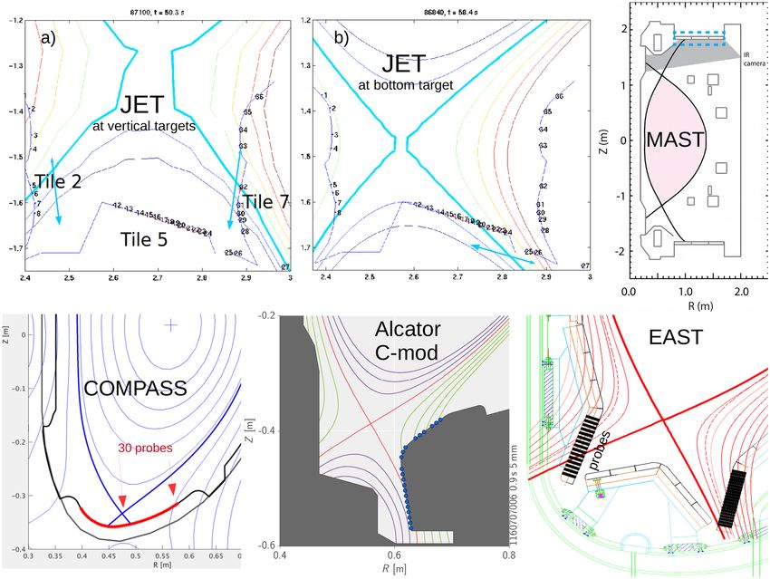
Figure 2. Divertor geometry, LCFS, dimensions and probe/IR cameras positions on the five analyzed tokamaks. JET, COMPASS, C-mod
and EAST are in the lower single-null divertor configuration while MAST runs a near-double-null configuration which is dominated by the
IR-observed top divertor.
the sheath-limited regime; if ν * > 15, it is in the conduction- 4. Main result: power decay length scaling
limited regime. This criterion applies to each flux tube indi- candidates
vidually, and so a part of the SOL may be sheath-limited
and a part conduction-limited. To account for this possible Figure 4(a),(b) shows the two previously published scalings
variation, collisionality was evaluated across the SOL using [10] and [2] applied to our new data set. When all our data
measurements of a reciprocating probe. T e was measured is included (that is, inner and outer targets, vertical and bot-
using the ball-pen probe and Langmuir probe technique [31]; tom horizontal targets and all tokamaks), only a small frac-
ne = jsat /0.5ecs , where e is the elementary charge and cs =
√ tion (R2 ) of its variation is described by the respective scalings.
2eTe /mi is the sound speed, was measured using a biased In contrast, the scaling [6] shown in figure 4(c) describes the
Langmuir probe and the aforementioned technique; finally L available database surprisingly well considering that it is based
was calculated from the equilibrium reconstruction as the con- on a single parameter ⟨p⟩, the volume-averaged plasma pres-
nection length of the OMP to the outer target. In the discharges sure, and its source data come solely from Alcator C-mod. We
where ν * > 15 over a majority of the SOL and > 10 across its included three more parameters alongside ⟨p⟩ to create scaling
entire extent, the overall SOL transport regime was judged to E8 in table 2 which describes our database very well (exclud-
be conduction-limited. Thus, the COMPASS data falls into ing unfortunately MAST due to lack of data).
two categories: either conduction-limited, or intermediate or To find a new scaling based on all our data, we employed the
sheath-limited. The choice between them is discussed in the methodology described in [15]. In contrary to many previous
following section. publications on tokamak heat flux scalings, e.g. [6, 2, 10–12],
Our results were cross-checked against the output of 2D we look for all possible combinations of∏scaling parameters,
N
slab OMP turbulence simulations by the code HESEL [3]. not a single one. We assume λomp q = α0 i=1 pα i
i . This trans-
∑ N
The simulations were set up for ASDEX Upgrade-like L-mode lates to log(λomp q ) = log(α0 ) + i=1 αi log(pi ) which allows
SOL parameters for a wide scan of relevant plasma conditions the standard (least-square) regression analysis. To limit the
(see the golden symbols in figures 3 and 4). For consistency, resulting number of possible scalings, we apply strong restric-
we related the code-relevant parameters as κ = 1.7, assum- tions on the scaling variables. The most prominent one is limit-
ing Bϕ = BLCFS a+R0R0 and q95 = qcyl because q95 has no direct ing the set of global plasma parameters to a set of 12: jp [A/m2 ],
meaning in this 2D model. Similarly, since ⟨p⟩ and β are not Bϕ [T], Bpol [T], ne [m−3 ], PSOL /SLCFS [MW/m2 ], ⟨p⟩[atm], β,
input parameters in HESEL, they are excluded from relevant fGw , q95 , qcyl , a/R0 , κ and δup . This was done based on the fol-
scalings. lowing considerations:
4Nucl. Fusion 60 (2020) 066016 J. Horacek et al
1 1 1
10 10 10
[mm]
omp
λ
0 0 0
10 10 10
0 1 −1 0 5 6
10 10 10 10 10 10
2
B [T] Bpol[T] jp[A/m ]
φ
1 1
1 10
10 10
λomp [mm]
0 0
0 10
10 10
−1 0 4 5
19 20 10 10
10 10 10 10
−3
ne[m ] [atm] 2
P /S [W/m ]
SOL LCFS
1 1 1
10 10 10
λomp [mm]
JET by probes at Inner Vertical
JET by probes at Outer Horizontal
JET by probes at Outer Vertical
COMPASS by probes at Outer
EAST by probes at Inner Vertical
MAST by IR at double−null Outer
HESEL simulation at outer midplane
0 0 0
10 10 C−mod by probes at Outer 10
0 2 4 6 8 0.2 0.3 0.4 0.5 0.6 0.7 −1
10
0
10
q a/R fGw
cyl
0
1
1 1 10
10 10
λomp [mm]
0 0 0
10 10 10
−3
10
−2
10 0 5 10 0.1 0.2 0.3 0.4 0.5
q δ
β 95 up
omp
Figure 3. Scan of the λq dependence on individual main plasma parameters as defined in table 1. The database includes five hundred
COMPASS (197), EAST(19), JET (113), Alcator C-mod (91) and MAST (88) L-mode divertor profiles obtained by either probes or IR
camera, as well as the output of 20 HESEL (2D slab turbulence) simulations. Dashed lines mark the parameters of ITER (yellow) and
COMPASS-Upgrade (blue). Note that there is no single-parameter scan; these are just projections of the 12-dimensional parameter space.
Note that the full database table of 550 entries of 47 parameters (only 12 used here) can be requested from horacek@ipp.cas.cz .
5Nucl. Fusion 60 (2020) 066016 J. Horacek et al
Table 1. Main plasma parameters of ITER [32] at t = 50 s and COMPASS-Upgrade [33] just before the L/H transition, calculated by
METIS simulations. Parameter type: engineering = very precise, global plasma parameter, dimensionless = theoretically determining the
plasma transport.
Unit Description COMPASS
Type Parameter definition just before L/H transition ITER Upgrade
e Ip MA Plasma current 12 2
e A m2 = πa2 κ cross-section 14.2 0.41
e jp = Ip /A MA/m2 Plasma current / cross-section 0.87 4.9
e Bϕ T Toroidal mag. field 5.3 5.0
e Bpol T Poloidal √
mag. field 1.14 1.03
= µ0 Ip /[2πa (1 + κ2 )/2]
e R0 m Major radius 6.5 0.89
e V m3 Plasma volume 576 2.3
g ne m−3 Line-averaged density 4 × 10¹⁹ 2 × 10²⁰
g PSOL MW Power
√ to SOL 18 3.7
g SLCFS m2 = 4π 2 R0 a (1 + κ2 )/2 surface 557 13.7
g PSOL /SLCFS MW/m2 Power through LCFS surface 0.033 0.27
g ⟨p⟩ = Epl /V atm = 101 kPa Plasma energy / volume = pressure 0.86 0.79
dg β ≡⟨p⟩2µ0 /B2ϕ Plasma / magnetic pressure 0.008 0.008
dg fGw ≡ 1020 Ipn/[π
e
a2 ] Greenwald density fraction 0.33 0.22
de q95 Safety factor at Ψ = 0.95 1.7 2.6
π a2 Bϕ (1+κ2 )
de qcyl ≡ µ0 I p R 0
Cylindrical safety factor 1.6 2.1
de a/R0 Minor/major radii 0.28 0.3
de κ ≡ b/a Vertical plasma elongation 1.4 1.8
de δup Upper plasma triangularity 0.21 0.49
• We exclude plasma elongation since it varies too weakly, Apart from constraining the overall global parameter set,
1.6 < κ < 2.0. further restrictions to the possible scalings are as follows:
• We normalise the parameters R0 , a, Ip , PSOL and Epl to jp =
Ip /A, a/R0, ⟨p⟩ = Epl /V and PSOL /SLCFS . This naturally • We require that all mutual cross-correlations Mcc between
excludes any extrapolation towards ITER and COMPASS- all the parameters used within each scaling are small
U (in accordance with [15]), as shown by the vertical lines enough:
∗
in figure 3 which all lie within the database span. Mcc < 2/3 across the entire database;
∗
• As previously done in [3, 34], we exclude all local separat- Mcc < 4/5 for each tokamak independently.
rix parameters which theoretically affect λomp q : the outer-
midplane separatrix temperature TeLCFS and density nLCFS e
This is imposed in order to avoid scaling ambiguity, since
or their peak divertor values Tepeak peak future tokamaks may not follow the same parameter correla-
,div and ne,div . There were
two reasons for this. One, their values for ITER cannot be tions. As a result, the number of scaling parameter combina-
reliably predicted without falling into self-consistent pro- tions is drastically reduced from 3000 down to a few dozens.
cedures, as ITER edge plasma modelling (e.g. in SOLPS- Furthermore, this requirement implicates that the scalings
ITER) generally uses λompq as input for the setup of its cross- have at maximum N≤4 parameters, otherwise some mutual
field transport coefficients. Two, the separatrix parameters correlation is too high.
values cannot be reliably measured in experiment either, as
the exact position of midplane separatrix is very question- • We require that each t−ratio = exponent
exponent αi
αi error > 3, meaning
able in current tokamaks. The typical systematic discrep- its statistical significance (the p-value) is above 99.9%.
ancy of 1 cm yields error of both Te LCFS and nLCFS values • We further require that all |αi | < 3, allowing for cubic
e
by a factor of exp(1 cm/λomp ) > 10. It was attempted on dependency at maximum.
q
COMPASS [35] and TCV [36] to identify the LCFS using • Finally, let us limit the number of best scalings by requiring
various techniques, yielding to systematic shift outwards the minimum regression quality R2 > 85%.
from the (EFIT or Liuqe) magnetic outer midplane separat-
Satisfying all the above restrictions yields 13 credible
rix by ≈2 cm on COMPASS and 0.5 cm on TCV. However,
scalings, listed in table 2 in black. The table also shows
even though this method seems more precise than the mag-
their predictions of λomp
q for ITER and COMPASS-U for L-
netic equilibrium reconstruction, it is not regularly used on
mode just before the L/H transition, using parameters from
tokamaks since it is quite complex and requires special dia-
table 1.
gnostics.
6Nucl. Fusion 60 (2020) 066016 J. Horacek et al
a) d) 2
R = 92%.
R2 =45%, R2 =40% Only outer targets
all outer 1
1 10
10
[mm]
λomp [mm]
omp
λ
0 0
10 10
0 1 1
10 10 10
−0.55 0.2 0.1
1.37⋅ B [T] P [MW] R [m] q1.17 2.8×10 ⋅ 3
(a/R )1.03 f0.48 2 −0.35
(j [A/m ])
φ SOL 0 cyl 0 Gw p
Eq.(7) in [T. Eich, J.Nuc.Mat. (2013)]
e)
b)
2
2 2 R = 88%.
Rall=59%, Router=69%
All tokamaks & targets
1
10 10
1
λomp [mm]
[mm]
λ
omp
0 0
10 10
0 1 1
10 10 10
1.58⋅ B [T]−0.4 P [MW] 0.13
q0.73 R [m]0.26 8.39⋅ Bφ[T]
−0.36 0.55 0.92
q95 fGw
φ SOL 95 0
Fig.5 in [A. Scarabosio, J.Nuc.Mat. (2013) S426]
c)
2 2
Rall=32%, Router=40%
Missing MAST JET by probes at Inner Vertical
1 JET by probes at Outer Horizontal
10
JET by probes at Outer Vertical
COMPASS by probes at Outer
λomp [mm]
EAST by probes at Inner Vertical
MAST by IR at double−null Outer
HESEL simulation at 2D outer midplane
C−mod by probes at Outer
predictions ITER,COMPASS−U
0
10
0 1
10 10
−0.48
0.91⋅ [atm]
C−mod scaling [D. Brunner Nucl. Fusion 58 (2018) 094002]
omp
Figure 4. Scalings of experimental values of L-mode divertor decay lengths λq with main plasma parameters. Predictions are shown by
the thick circle: yellow for ITER and blue for COMPASS-Upgrade. Inner targets and HESEL simulation are less credible (marked by light
symbols). (a) P1 according to [2] (b) P2 according to [10], both derived from ASDEX Upgrade and JET only, (c) P3 according to [6]
(derived from Alcator C-mod only). Examples of best NEW scalings based on (d) only outer targets D1, (e) all tokamaks F1.
5. Discussion of the scalings COMPASS, only discharges with conduction-limited SOL
were used. MAST data were excluded, as well as data
To investigate the robustness of the derived scaling laws, we obtained at inner targets (which may scale differently).
split the λomp
q database into six datasets: • Dataset B contains dataset A as well as the data from
MAST, allowing to asses the role of near-double null plas-
• Dataset A keeps only the most conservative (credible) data mas and different aspect ratios. Note, however, that both
obtained from the measurements at the outer targets. For influences are present in the MAST data simultaneously.
7Nucl. Fusion 60 (2020) 066016 J. Horacek et al
• Dataset C containes dataset A as well as all the COMPASS at AUG [37], where the λomp q measured at the inner target
data to assess the role of SOL transport. exhibited dependence on different parameters than measure-
• Dataset D contains data from outer targets of all the studied ments at the outer target. The second matter of interest is that,
tokamaks. surprisingly, scalings derived from dataset E also contain a
• Dataset E contains data from both the inner and the outer dependence on the aspect ratio a/R0 , although the variation of
targets but excludes MAST, allowing to asses the possibly this parameter is not great in the absence of MAST data. This
different scaling of λomp
q at the inner target. is demonstrated by many cross-group R2 < 0, marked by the
• Dataset F contains all the data. red color pointing to poor predictive capability of such scal-
ings. This is because the a/R0 exponent is always negative
Table 2 lists the scalings which match the criteria described where MAST data is included. This is most probably caused
in section 4 for each respective dataset. The second column by the presence of data from the inner target of EAST, which
shows the coefficient of determination R2 meaning “what per- has a slightly smaller aspect ratio than other tokamaks in the
centage of the data variation is explained/described by the scal- dataset. This suggests two conclusions: (i) the scaling of λomp q
ing”. Each scaling was tested against each of the six datasets. at the inner target is indeed more complicated than the one
The R2 corresponding to its own dataset is marked in a large at the outer target, and (ii) the aspect ratio is probably not
font and bold face. a very reliable scaling parameter, which may be caused by
For the most conservative dataset A, only one scaling A1 the hidden dependencies on other parameters (as mentioned
was found, with relatively red poor fit quality R2 = 77%. This earlier).
is mostly due to the relatively small range of λomp q caused by Consequently, we have attempted to derive a scaling based
excluding MAST data, which generally show large values of on dataset E which would contain a dependence on the aver-
λomp
q as seen in figure 3. The same problem befalls scaling aged plasma pressure, which is the principal parameter iden-
C1. When the MAST data are added (dataset B), the scaling tified by Brunner [6]. The quality of such fit is decent and
B1 with excellent fit quality R2 = 92% is obtained. However, the ⟨p⟩ exponent –0.44 is very similar to the one obtained
note that one of the scaling parameters is the aspect ratio a/R0 , by Brunner (–0.48). However, two more parameters appear to
which has limited variation on all tokamaks except for MAST be significant—the aspect ratio and β. The inclusion of β is
(see figure 3). In principle, this parameter may not be itself caused by the data from COMPASS, which were obtained at
responsible for the variation of λomp
q but serves as a proxy for significantly higher values of β than on other tokamaks.
some other parameter, which is different on this spherical toka- Finally, when all the available data are used (dataset F), the
mak. Nevertheless, the aim of our work is not to uncover the fit quality decreases slightly compared to the more restricted
underlying physics which determines the scaling of λomp q but datasets. The best quality scaling F1 depends on Bϕ , q95 and
to provide a reliable prediction based mostly on parameters f Gw . The safety factor includes a dependence on the poloidal
which are straightforward to determine. magnetic field, but the exponent is different from the H-mode
When all data obtained at the outer targets are used (dataset scaling derived by Eich [2]. The significant dependence on fGw
D), the dataset becomes sufficiently robust to yield a number does not appear in the H-mode scalings either. This may be
of scalings with good fit quality. Some of them (D7, D0), how- caused by the generally larger variation of fGw in L-mode plas-
ever, perform poorly when applied to the more restricted data- mas in our datasets. In H-mode, it is difficult to achieve meas-
sets (having large negative R2 ) and are therefore excluded from urements below the natural H-mode density or even to enter
further considerations. Note that a majority of these scalings H-mode at such conditions, since the L-H power threshold is
exhibit a similar dependence on f Gw , with the exponent value known to increase sharply in such a case. Moreover, high dens-
in the range of 0.5–0.9. Such dependence was not observed in ity discharges are usually not analysed when IR thermography
the published scalings P1-4, although it may have been to some is employed as the principal diagnostic, which was the case
extend included in the dependence on pressure. All the cred- in [2], due to the parasitic influence of bremsstrahlung. There-
ible scalings also depend approximately linearly on the aspect fore, the dependence on f Gw may have appeared as insignific-
ratio, similarly to the dependence found in dataset B. ant in such studies.
When data from outer and inner targets are combined (data- Note that scaling F1 (which has the highest R2 for this data-
set E), it is possible to derive credible scalings even without set) does not employ the aspect ratio, however the λomp q pre-
the contribution of MAST data. We address three particular dictions for ITER and COMPASS-U are quite similar to those
interesting aspects of these scalings. Firstly, the upper triangu- obtained with scaling F2, where the aspect ratio is included.
larity δ up appears as a significant parameter. This was not the This suggests that although the role of aspect ratio is probably
case in the previous datasets, even though they contained data quite complex, it is not essential for determination of λomp q in
with a significant range of δ up (such as the C-mod data). This the cases of our interest.
suggests that δ up influences the transport to the inner target. Two observations may be made across the datasets. Firstly,
Following the conventional picture of transport in the SOL, most of the credible scalings use one (and only one) of
with the blob source in the vicinity of the outer midplane and the parameters Bϕ , Bpol , jp , qcyl and q95 . This is to be expec-
subsequent parallel transport along the open field lines, it may ted since they are all naturally correlated within the data-
imply that the location on the top of the tokamak (where the base. Secondly, the R2 is not significantly modified when
plasma shape is strongly influenced by δ up ) plays a key role in HESEL results are included in the fit, which leads us to
this process. This conclusion is consistent with observations the conclusion that HESEL is generally in good agreement
8Nucl. Fusion 60 (2020) 066016 J. Horacek et al
omp
Table 2. The most credible scalings for each dataset, ordered by the coefficient of determination R2 . The λq predictions are based on the
parameters listed in table 1. Note that this METIS ITER scenario has very low q95 < 2 which is probably MHD unstable. We verified that a
more realistic ITER scenario with q95 = 2.2 (due to faster shaping) yields predictions with λomp q longer (peak heat flux smaller) by 10% for
half of the scalings. R2ABCDEF for all the datasets are shown on the left. R2 of the dataset which was used to derive the respective scaling is
marked as R2withoutHESEL /R2includingHESEL . Red-colored scalings which have R2 < 85% for all the datasets or have R2 < 0 for any one dataset
are not considered credible. Note that scaling E8, based on the average pressure, yields significantly shorter λomp
q for ITER and
COMPASS-U. qpeak ⊥ is estimated according to equation (3). Further marked are the Eng.ineering scalings which use only highly credible
inputs, independent from (uncertain) plasma conditions.
R2 [%] ITER Compass-U ITER Compass-U
fit quality λomp
q λomp
q qpeak
⊥ qpeak
⊥
# ABCDEF Scaling formulas mm mm MWm−2 MWm−2
A: conduction
limited outer targets w/o MAST
A1 77/77,77,33,33,20,20 1.82 · q− 95
0.43
< p > [atm]−0.48
1.5
1.4 2
0 3
3
B: = A + MAST
0.55 −0.37
B1 79,92/90,66,92,42,71 4.03 × 10³ · (a/R0 )1.06 fGw jp 3.3 1.5 9.4 29
C: = A + all COMPASS
C1 76,69,62/51,74,-32,26 −0.52
1830 · qcyl (a/R0 )1.29 (PSOL /SLCFS )−0.4
4.3
1.7
7.3 2
6
D: All outer targets (with MAST)
.48 −0.35
D1 79,92,67,92/91,42,71 2800 · (a/R0 )1.03 f0Gw jp 3.5 1.7 9 27
−0.19 0.27
D2 53,90,34,91/90,31,67 27.5 · Bϕ qcyl (a/R0 )1.11 f0Gw .71
2.5 2.3 13 20
−0.23
D3 58,90,38,91/90,32,67 28.5 · Bpol (a/R0 ) fGw 1.25 0.7
2.6 2.2 12 20
D4 61,89,50,91/90,6,55 195 · (a/R0 )1.48 (PSOL /SLCFS )−0.14 f0Gw .62
3.4 2.2 9.2 20
D5 22,88,15,89/88,16,60 38.4 · qcyl (a/R0 ) fGw
0.22 1.5 0.66
3 2.8 11 16
D6 55,88,40,89/86,17,59 32.8 · B−ϕ
0.15
(a/R0 )1.08 f0Gw .64
3.1 2.7 10 17
D7 64,91,-6,88/87,79,87 −0.4 0.48 0.87
8.64 · Bϕ q95 fGw
2.1
1.9 1
5 2
3
D8 32,86,26,88/85,7,55 42 · (a/R0 )1.41 f0Gw .61
3.5 3.1 8.9 15
1.09 −0.43
D9 80,85,67,87/82,22,59 Eng. 4350 · (a/R0 ) jp 3.1 1.6 10 28
D0 62,90,-27,87/87,64,80 13.9 · B− ϕ
0.6 0.23 0.86
qcyl fGw
2.2
1.7 1
5 2
6
E: = C + inners = all w/o MAST
E1 85,-34,72,-11,92/92,8 5690 · δup
0.25
(a/R0 )−0.9 f0Gw .27 −0.56
jp
4.1
1.7
7.6 2
7
E2 83,-99,72,-64,91/89,-35 961 · (a/R0 ) −1.41 0.24 −0.5
fGw jp
4.5
1.5 7 3
0
0.45 0.34 −0.6
E3 83,78,68,81,90/90,82 44000 · δup fGw jp 3.7 1.7 8.4 26
E4 84,-56,69,-26,89/89,-5 Eng. 9070 · δup (a/R0 )−1.12 jp−0.64
0.21
4
1.5
7.8 3
1
E5 83,-100,70,-65,89/85,-36 Eng. 2040 · (a/R0 )−1.52 j− p
0.59
4.3
1.4
7.3 no
0.46 −0.73
E6 81,77,64,81,85/85,80 Eng. 1.48 × 10 · δup jp
5
3.5 1.5 9 30
E7 24,-120,8,-80,85/85,-48 2.8 · (a/R0 )−1.37 f0Gw .97
5.4
3.4
5.8 1
3
E8 73,73,55,55,88/88,88 0.024 · < p > [atm]−0.44 (a/R0 )−1.96 β −0.27 1.2? 1.1? 27? 43?
F: All tokamaks and targets
F1 62,90,-14,88,83,88/85 8.39 · Bϕ−0.36 q095.55 f0Gw.92
2.2 2 1
4 2
3
−0.2 0.52
F2 52,90,7,89,77,85/83 12.1 · Bϕ q95 (a/R0 )0.42 f0Gw .9
2.5 2.3 13 20
F3 12,87,-14,87,72,83/80 15 · q95 (a/R0 ) fGw
0.59 0.78 0.89
2.8
2.7 1
1 1
7
Published scalings
P1 46,23,27,38,77,77,44/42 [2, equation 7]: 1.37 · B− ϕ
0.55 0.2 1.17 0.1
PSOL qcyl R0 2.0 1.8 16 26
−0.4 0.13 0.73 0.26
P2 62,60,54,68,55,57/52 [10, figure 5]: 1.58 · Bϕ PSOL q95 R0 2.9 1.9 11 24
P3 65,65,40,40,32,32/32 Scaling [6]: 0.91 · ⟨p⟩−0.48
1.0
1.0 3
2 4
4
P4 R2 < 0 [27]: 3.12 × 10⁻²⁹ · B− 0.63 1.45 −0.19 1.45
ne PSOL q95
0.36
9.5 8
7
4.8
ϕ
P5 R2 < 0 0.59 1.21 0.61 −0.19 0.54
[9][p.589] L-1: 0.66 · q95 R0 Zeff Pdiv ne 1
4
5.4
2.2
8.5
P6 R2 < 0 [9][p.589] L-2: 0.72 · q095.59 R10.21 Z0eff.65 P− 0.28 0.68
SOL ne 1
4
7.6
2.2 6
P7 R2 < 0 [8, p.2423]: 3.2 · q095.53 Z0eff.56 P− 0.76 0.91
n e
2.6
4 7
12
0.98
div
with all the (black-marked) scalings (see the yellow stars in is not surprising as it is based on a single parameter and
figure 4). derived from a single tokamak. Generalized version of P3 is
Concerning the Published scalings, even though R2 ≈ 12 the scaling E8 with R2 = 88%, however, they both predict (for
for P1–P2, we consider them credible since they were derived unknown reasons) significantly smaller λomp
q than all the other
from a fully different dataset (from 2013 Asdex-Upgrade and 15 scalings (not based on ⟨p⟩).
JET) than tested here. We consider P3 as marginally credible In contrary, all the scalings P4–P7 do not describe/predict
because it describes only 32% of the data variation, which well our database. The scalings P5-7 from year 1999 JET +
9Nucl. Fusion 60 (2020) 066016 J. Horacek et al
JT-60U contain ne /1019 and the unknown parameters we 7. Conclusion
approximated as Zeff = 1.5, Pdiv = 43 PSOL , however, those
assumptions do not influence the following judgements. The In order to improve the existing scalings of the SOL power
scalings P5–6 match reasonably both COMPASS and EAST, width λompq such as [2] and [10], we have measured, analyzed
overestimate JET and HESEL by factor of two and fails com- and combined five hundred COMPASS, Alcator C-mod [6],
pletely for MAST and C-mod. The scaling P7 overestimates EAST [7], JET and MAST L-mode divertor heat flux pro-
by factor of two MAST, EAST and JET, however, fails (over- files obtained by either probes or IR camera as well as out-
estimates by factor of 10–20) C-mod, COMPASS and HESEL. put from HESEL (2D slab turbulence) simulations [3] using
In conclusion, we point out that despite the different settings based on tokamak ASDEX Upgrade parameters. To
scaling parameters and underlying datasets, all 15 cred- assess the coherence of our heterogeneous database, we split
ible scalings in table 2 (set in black) predict very similar it into six overlapping datasets and applied stringent criteria to
values of λomp
q for ITER, 3.0 ± 0.5 mm, and COMPASS- the resulting scalings. This allowed us to reduce the possible
U, 2.1 ± 0.5 mm. This validates our approach to seek ~3000 scalings to just 24 scalings, which are listed in table 2,
all possible scaling laws in order to asses the result each with very high credibility (describing 85–92% of the data
robustness. variability). Further testing showed that only half of those new
scalings had strong predictive capabilities outside their ”nat-
ive” datasets.
6. Implied estimate of peak heat flux Our main result is that just before the L-H transition, all the
13 credible scalings (as well as [2] and [10]) yield consist-
Following [38], λompq determines the effective divertor wetted ent predictions of λq omp for both ITER and COMPASS-
area as Adw = ftw 2πR0 λint fx , where ftw is the toroidal wetted Upgrade:
fraction [39], λint ≈ λomp
q + 1.64S is the integral power decay
length and f x is the poloidal magnetic flux expansion between • λomp
q ITER = 3.0 ± 0.5 mm when using all reasonable para-
the OMP and the divertor. meter combinations. Note that this prediction is quite sim-
We further assume that: ilar to the Q = 10 burning DT ITER H-mode [41, figure 4].
• λomp
q COMPASS − U = 2.1 ± 0.5 mm.
• both targets receive an equal amount of power,
• negligible energy is radiated in the SOL, and thus the It must be noted, however, that one of the 13 scalings (E8,
plasma is fully attached, based on the average plasma pressure ⟨p⟩, not available for
• no power is lost to the first wall since λomp
q is much smaller MAST) yields a significantly shorter λomp
q = 1.1 − 1.2 mm for
than the separatrix-wall distance, both tokamaks and that the reason is currently unknown.
• the heat flux does not spread into the private flux region, We suggest that predictions of tokamak divertor conditions
S = 0 and λint = λomp
q , be done using as many black-colored scalings from table 2 as
• the OMP-to-divertor poloidal magnetic flux expansion is possible, excluding those in red color.
f x = 9, and For an attached L-mode plasma all the scalings yield (using
• the toroidal wetted area fraction is ftw = 0.8. significant assumptions from section 6) divertor surface-
perpendicular peak heat flux qpeak ⊥ITER ≈ 10 MW/m
2
and
Under these assumptions, Pdivertor ≈ PSOL /2 and the result- peak
q⊥COMPASS−U ≈ 20 MW/m2 .
ing surface peak heat flux on two strike points is
qpeak
⊥ ≈ PSOL / (2Adw ) (3)
Acknowledgments
The resulting predictions of qpeak
⊥ for ITER and COMPASS- This work was supported by projects Czech Science
U are shown in the right column of table 2. In the case of Foundation Grant GA19-15229S, MEYS LM2015045,
ITER, we consider the baseline scenario with plasma condi- EF16_013/0001551, US DoE cooperative agreements DE-
tions just before the L-H transition (see table 1), using the SC0014264 and DE-FC02-99ER54512 on Alcator C-Mod, a
respective predicted value of λqomp and the expected value of DoE Office of Science user facility. This work has been carried
PSOL . Note that from the point of view of the machine pro- out within the framework of the EUROfusion Consortium and
textion, the ITER divertor should keep the surface temperat- has received funding from the Euratom research and training
ure of its water-cooled monoblocks below the cyclical damage program 2014-2018 and 2019-2020 under Grant Agreement
limit (recrystallization), which corresponds to the steady-state No. 633053. This work has been carried out within the frame-
−2
heat load qpeak
⊥ ≤ 10 − 15 MW m [40]. This should prevent work of the Contract for the Operation of the JET Facilities
damage to the divertor monoblocks also in case when the L- and has received funding from the European Union’s Horizon
H transition could not be achieved for some reason and the 2020 research and innovation program. The views and opin-
L-mode phase would extend on the timescale of the thermal ions expressed herein do not necessarily reflect those of the
response of the monoblocks. In case of COMPASS-U [33], European Commission. I acknowledge M. Bernert and J.F.
we consider the scenario with the most demanding parameters Artaud for significant help, R. Dejarnac, T. Eich, B. Sieglin
(I p = 2 MA, Bϕ = 5.0 T). and A. Scarabosio for discussing the JET probes analysis.
10Nucl. Fusion 60 (2020) 066016 J. Horacek et al
ORCID iDs [16] Kocan M. et al 2015 Nucl. Fusion 55 033019
[17] Vondracek P. 2019 Plasma Heat Flux to Solid Structures in
J. Horacek https://orcid.org/0000-0002-4276-3124 Tokamaks PhD Thesis (University of Prague)
[18] Guillemaut C. et al 2015 Plasma Phys. Control. Fusion
J. Adamek https://orcid.org/0000-0001-8562-1233
57 8 085006
P. Vondracek https://orcid.org/0000-0003-0125-9252 [19] Adamek J. et al 2017 Nucl. Fusion 57 116017
G. Deng https://orcid.org/0000-0001-6940-0043 [20] Vondracek P. 2018 Plasma Heat Flux to Solid Structures in
X. Gao https://orcid.org/0000-0003-1885-2538 Tokamaks Dissertation PhD thesis Charles University
D. Brunner https://orcid.org/0000-0002-8753-1124 Prague (https://is.cuni.cz/webapps/zzp/detail/123000/)
[21] Vondracek P. et al 2019 Fusion Eng. Des. 146 1003–6
B. LaBombard https://orcid.org/0000-0002-7841-9261
[22] Hermann A. et al 1995 Plasma Phys. Contr. Fusion 37 17
A.H. Nielsen https://orcid.org/0000-0003-3642-3905 [23] Efron B. and Tibshirani R.J. An Introduction to the Bootstrap
M. Ezzat https://orcid.org/0000-0001-9894-009X (London: Chapman and Hall)
[24] Brunner D. et al 2018 Nucl. Fusion 58 076010
[25] Sun H.J. et al Plasma Phys. Control. Fusion 2015 57 125011
References [26] Lipschultz B. et al 1995 J. Nucl. Mater. 220–222 50–61
[27] Ahn J.-W. et al 2006 Plasma Phys. Control. Fusion 48 1077
[1] Eich T. et al 2011 PRL 107 215001 [28] Chen Y.P. et al 2011 J. Nucl. Mater. 415 S517–S522
[2] Eich T. et al 2013 J. Nucl. Mater. 438 S72–S77 [29] Silva C. 2000 Divertor physics studies on COMPASS-D.
[3] Olsen J. et al 2018 Plasma Phys. Control. Fusion 60 085018 Dissertation Thesis Technical University of Lisbon
[4] Halpern F.D. et al 2016 Plasma Phys. Control. Fusion [30] Stangeby P.C. 2000 The Plasma Boundary of Magnetic Fusion
58 084003 Devices (Boca Raton, FL: CRC Press)
[5] Tsui C. et al 2018 Phys. Plasmas 25 072506 [31] Dimitrova M. et al 2017 Plasma Phys. Control. Fusion
[6] Brunner D. et al 2018 Nucl. Fusion 58 094002 59 125001
[7] Deng G.Z. et al 2018 Plasma Phys. Control. Fusion [32] Artaud J.F. et al 2018 Nucl. Fusion 58 105001
60 045001 [33] Panek R. et al 2017 Fusion Eng. Des. 123 11–16
[8] ITER physics basis 1999 Chapter 4: Power and particle control [34] Nielsen A.H. et al 2019 Nucl. Fusion 59 086059
Nuclear Fusion 39 2391 [35] Seidl J. et al 2017 Nucl. Fusion 57 126048
[9] Loarte A. et al 1999 J. Nucl. Mater. 266–269 587–92 [36] Tsui C. et al 2017 Phys. Plasmas 24 062508
[10] Scarabosio A. et al 2013 J. Nucl. Mater. 438 S426–S430 [37] Faitsch M. et al 2015 Plasma Phys. Control. Fusion 57 075005
[11] Sieglin B. et al 2016 Plasma Phys. Control. Fusion [38] Makowski M. et al 2012 Phys. Plasmas 19 056122
58 055015 [39] Pitts R.A. et al 2017 Nucl. Mater. Energy 12 60–74
[12] Elmore S. et al 2018 Scaling of the scrape-off layer width in [40] De Temmerman G. et al 2018 Plasma Phys. Control. Fusion
MAST L-mode plasmas as measured by infrared 60 044018
thermography 45th EPS Conf. Plasma Physics (Prague, [41] Pitts R.A. et al 2019 Nuclear Materials and Energy 20 100696
Czech Republic, 2–6 July 2018) P1.1027 [42] Eich T. et al 2018 Nucl. Fusion 58 034001
(http://ocs.ciemat.es/EPS2018PAP/pdf/P1.1027.pdf) [43] Marsen S. et al 2013 Divertor heat load in JET – comparing
[13] Horacek J. et al 2015 J. Nucl. Mater. 463 385–8 langmuir probe and IR data 40th EPS Conf. Plasma Physics
[14] Goldston R.J. 2012 Nucl. Fusion 52 013009 (Espoo, Finalnd, 1–5 July 2013) P1.127
[15] Horacek J. et al 2016 Plasma Phys. Control. Fusion (http://ocs.ciemat.es/EPS2013PAP/pdf/P1.127.pdf)
58 074005 [44] Aftanas M. et al 2012 Rev. Sci. Instr. 83 10E350
11You can also read