Macroeconomic Effect on the Automobile Sales in Top Four Automobile Production Countries - kosbed
←
→
Page content transcription
If your browser does not render page correctly, please read the page content below

KOSBED, 2018, 35: 139 - 161
Yayın Geliş Tarihi: 03.01.2018
Macroeconomic Effect on the
Yayın Onay Tarihi: 04.04.2018 Automobile Sales in Top Four
Automobile Production Countries
Ferhat PEHLİVANOĞLU
Retno RİYANTİ
En Büyük Dört Otomobil Üreticisi Ülkedeki Araç
Satışlarının Makroekonomik Etkileri
Abstract
The automotive industry is a major industrial and economic force worldwide. This paper examines
macroeconomic effect with six variables on the automobile sales in top four automobile production
countries. These variables are real GDP, GDP per capita, automobile production, inflation, gasoline
price, and exchange rate; and the countries has been selected are China, USA, Japan, and Germany
that has first four highest automobile production countries in the world. The findings shows that
real GDP, car production, gasoline price have positive impact towards car sales while change in
GDP percapita, inflation and exchange rate cause the opposite. Some variables in this research
based on findings is inconsistent with the previous findings done by other researcher. While for
those top countries GDP percapita and gasoline price have different effect to the automobile sales.
The reason of that situation is because GDP percapita that reflect fluctuation of income perpeople
of those countries have no significant effectto the number of automobile sales.
Anahtar Kelimeler: Automobile Sales, Real GDP, Automobile Production, Gasoline Price.
JEL Codes: E23, F14
Özet
Otomotiv endüstrisi dünya genelinde önemli bir sanayi kolu ve ülkeler için ekonomik bir güçtür.
Bu çalışmanın amacı altı değişkenin otomobil üretimi üzerindeki makroekonomik etkisini
incelemektir. Söz konusu değişkenler; reel GSYİH, kişi başı GSYİH, otomobil üretimi, enflasyon
oranları, benzin fiyatları ve döviz kurudur. Çalışmanın analiz kısmı için seçilen ülkeler ise Çin,
ABD, Japonya ve Almanya'dır. Bu ekonomiler dünyada otomobil üretiminde en büyük pay sahibi
ilk dört ülkedir. Çalışma bulgularına göre, reel GSYİH, otomobil üretimi ve benzin fiyatlarının
otomobil satışları üzerinde olumlu etkileri olduğunu gösterirken, kişi başı GSYİH, enflasyon ve
döviz kuru tam tersi olarak üretim üzerinde olumsuz etkiler göstermiştir. Bu çalışmadaki bazı
Assoc. Prof, Kocaeli University, Faculty of Economics and Administrative Sciences, Department of
Economics, fpehlivanoglu@kocaeli.edu.tr
Master Student, Kocaeli University, Social Sciences Institute, Department of Economics,
retno.riyanti@gmail.com
This article is produced from a master thesis called " Competitive Advantage of Automotive
Industry in The Emerging Market Economies Countries in Term of Comparison "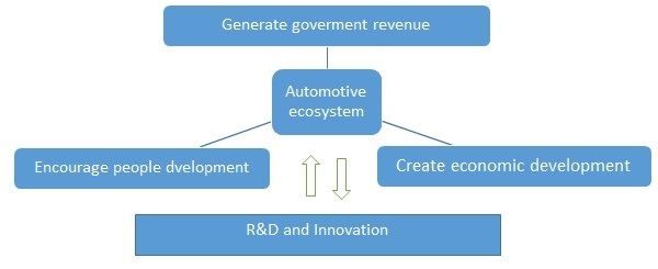
140•Kocaeli Üniversitesi Sosyal Bilimler Dergisi, KOSBED, 2018, 35

değişkenlerin otomobil satışı üzerindeki etkileri literatürdeki diğer bazı çalışmalara göre çelişen
sonuçlar göstermiştir. Örneğin bu üst düzey ülkeler için kişi başı GSYİH ve benzin fiyatlarının
otomobil satışları üzerinde farklı etkileri vardır. Bu durumun nedeni, söz konusu ülkelerin her
birinin kişi başına düşen gelir düzeylerinin büyük dalgalanma göstermesidir.

Keywords: Otomobil Satışları, Otomobil Üretimi, Benzin Fiyatları

JEL Kodları: E23, F14

    Introduction

    Transportation is one of the most essential economic goods in the modern world. An
efficient mode of transportation ensures the mobility of individuals and product delivery
could be conducted in a safe and timely manner. To meet this requirement, various types
and models of vehicles were produced by automotive companies to fulfil the needs of
consumers especially in the context of passenger vehicles.

    The automobile is a pillar of the global economy, a main driver of macroeconomic
growth and stability and technological advancement inboth developed and developing
countries, spanning many adjacent industries. The core automotive industry (vehicle and
parts makers) support wide range of business segment, both upstream and downstream,
along with adjacent industries (figure 1).

    Figure 1.The Core Automotive Industry Supports Upstream And Downstream
Industries
Macroeconomic Effect on the Automobile Sales in Top Four Automobile Production Countries • 141
Automotive contributes to several important dimensions of nation building:
generating government revenue, creating economic development, encouraging people
development, and fostering R&D and innovation (figure 2).
Figure 2.The Auto Industry’s Contribution To The Economy
Generating revenue. The automotive sector contributes significant tax revenues from
vehicle sales, usage-related levies, personal income taxes, and business taxes. Production
and sales of new and used vehicles, parts, and services deliver excise, sales, value-added,
and local taxes and import duties.
Economic development.The automotive industry is important to global economic
development.Globally, automotive contributes roughly 3 percent of all GDP output; the
share is even higher in emerging markets, with rates in China and India at 7 percent and
rising.
People development.Worldwide there is one motor vehicle for every five people; in
the United States there is one car for every 1.25 citizens. Automobiles can increase quality
of life through increased mobility, comfort, and safety.
Fostering R&D and innovation.R&D investment by automakers is driven by
consumer demands for more product variety, better performance, improved safety,
higher emission standards, and lower costs.
1. Automotive Market
Four main markets dominate global car sales are China, the United States, Germany,
and Japan. China has been the largest market since 2009, and its lead over the United
States is growing with each dominant market in terms of passenger car sales, emerging142•Kocaeli Üniversitesi Sosyal Bilimler Dergisi, KOSBED, 2018, 35
markets are yet to impose themselves in terms of sales volumes. The hoped-for El Dorado
is struggling to materialize as economic and political crises slow household vehicle
ownership rates.
Car sales by market reflect the economic difficulties facing various countries. The
recovery is sluggish in Europe; in the United States it is more pronounced, but “jobless”;
in Japan it is underpinned by public policies; in the emerging countries it is lagging
behind. despite high expectations. Car registrations are also a major indicator of a
country’s economic health. This report sheds light on their expected trends.( Economic
Outlook, 2014: 5)
Growth in global automotive production is likely to remainat around +4% per year
in2014 and 2015, with anincrease in production inChina, India, and Mexico at theexpense
of Europe. Productionis even expected to exceed100 million vehicles by 2017.The major
componentmanufacturers, which areessential for auto makers,have relocated to
followproduction and registerhealthy levels of profitability.( Economic Outlook, 2014:8)
Global new automobile sales totaled 20.44 million units during the first quarter of
2016. That is 2.8% more than the total posted in Q1 2015, or 558,700 more units. The
biggest contributors to this growth were the Chinese and European markets, both of
which continued to show positive macroeconomic trends. Meanwhile the US car market
moderated its growth, whilst Japan, Brazil and Russia recorded the biggest drops.(JATO,
2016:16) By JATO Dynamic Limited has summarized to identify countries which have
high influence to the world automobile market (Table 1).
Table 1.Top Ten Automobile Markets 2016-Q1
Countries Units (000) Change Q1 (2015-2016)
China 6.073 +6%
USA 4.081 +3%
Japan 1.449 -7%
UK 871 +5%
Germany 849 +5%
India 807 +3%
France 616 +8%
Italy 558 +21%
Brazil 465 -28%
South Korea 416 +5%Macroeconomic Effect on the Automobile Sales in Top Four Automobile Production Countries • 143 Source: JATO Dynamics Limited With growth of +10% in 2014 and +8% expected for 2015, the Chinese market is extending its lead after having surpassed overtaken the US market in 2009. At nearly 20 million units sold in 2014, it now accounts for 27% of global sales. Moreover, with an ownership rate of close to 5%, it offers all auto makers very attractive prospects for long- term growth of around +8% to +10% per year. It is a vehicle market whose role is growing: with 21 million units sold in 2015, it will be 25% larger than the US market. The US market represents 23%of global sales of passengervehicles (PV) and light commercialvehicles (LCV), or 16.5million unitsIt has become very profitable onceagain, after the deep restructuringscarried out in 2009-2010. The USautomotive industry has thus regainedthe competitiveness it hadpreviously lost: for an unchangedlevel of production, the workforcehas been reduced by -20% andmany production sites have beenshut down. Armed with a renewedand completely restructured productrange, US groups have returnedto being profitable, although forGeneral Motors 2014 will be largelytarnished by massive callbacks ofits vehicles (nearly 25 million) forsafety reasons. The automotive industry is one of the Japanese economy’s core sectors, in 2013 automotive shipments accounted for 17.8% of the total of Japan’s manufacturing shipments, and 40.9% of the value of the machinery industries combined shipments.(JAMA, 2015:22)The production of passenger vehicles by Japanese manufacturers in 2014 saw a slight increase of 1.1% compared to the previous year to total of 8.2 million units. In 2014 motor vehicles in Japan increased for the first time in two years, totaling 9.77 million units, up 1.5% from the previous year. German automobile manufacturers produced over 15 million vehicles in 2015that equivalent to more than 19 percent of total global production. 21 of the world’s 100 top automotive suppliers are German companies. Germany is the European car production leader: some 5.7 million passenger carsand 325.200 trucks and buses were manufactured in German plants in 2015. The automotive industry is the largest industry sector in Germany. In 2015, the auto sector recorded turnover of EUR 404 billion which is around 20% of the total German industry revenue. (GTAI, 2017:18)
144•Kocaeli Üniversitesi Sosyal Bilimler Dergisi, KOSBED, 2018, 35

      2.   Macroeconomic Report of the Countries
      2.1. China

    According to the World Bank, the Gross Domestic Product of China was 10351.11
billion USD in 2014, rank 2 globally. The GDP per capita was 7587.29 USD positioning
China at rank number 77 in the world in terms of economic development.Foreign direct
investment into China was 268.10 billion USD in 2014 which is 2.59 percent of GDP. We
look primarily at the percent of GDP as opposed to the dollar amounts because larger
economies would normally attract greater volumes of foreign investment. Values above
4-5 percent of GDP suggest that the country is an attractive foreign investment
destination.

    China is one of the main (top 10) trading partners of more than 100 economies that
account for about 80 percent of world GDP. Given is key role in global and regional
supply chains-importing intermediate and capital goods and exporting processed goods -
China can also be a conduit for shocks that originate in other countries. Furthermore,
over the past decade, China’s role as a source of final demand has increased markedly:
china’s imports of final capital goods and consumption goods from Europe and the
United State are material. IMF staff analysis suggest that a 1 percentage point investment-
driven drop in China’s output growth would reduce Group of Twenty (G20) growth by
¼ percentage point.

    China’s economic growth has proved to be quite resilient. At 6.9 percent for the whole
year, the country’s GDP growth rate for 2015 stayed very much in line with the official
target. While slower than previous years, this is still among the highest of the world’s
major economies, and given the size of China’s economy today, the increase in economic
output in 2015 was more than in previous years when the growth rate was higher. In
comparison, the US would have to grow at 4 percent in order to produce the same
amount of incremental economic output that China generated with 6.9 percent growth.
Unsurprisingly, according to forecasts prepared by the International Monetary Fund
(IMF), China is expected to continue being the largest contributor to world GDP – in
purchasing power parity terms – and is expected to account for nearly 20 percent of
Macroeconomic Effect on the Automobile Sales in Top Four Automobile Production Countries • 145
world GDP by 2020, compared to 15.5 percent for the European Union and 14.9 percent
for the US.(IMF, 2015)
China, now the world’s largest economy on a purchasing power parity basis, is
navigating a momentous but complex transition toward more sustainable growth based
on consumption and services. Ultimately, that process will benefit both China and the
world. Given China’s important role in global trade, however, bumps along the way
could have substantial spillover effects, especially on emerging market and developing
economies.
2.2. United States of America
Seven yearsafterfinancial crisis, the United States comeback with economic recovery,
while modest by historical standards, has been one of the strongest in the OECD, by
robust monetary policy support and an early expansion. Many sector jobs have been
created,about 2.6 million jobs in 2015, pushing unemployment down to its pre-crisis level
fell to 5.0 percent, half its level in fall 2009, thereby providing consumers with higher
income and improving their confidence. Health care price growth remained at low levels
not seen in nearly five decades as the Nation’s uninsured rate fell below 10 percent for
the first time ever. (OECD, 2016)
The US economy continued to grow in 2015, as the recovery extended into its seventh
year with widespread growth in domestic demand, strong gains in labor markets and
real wages, and low inflation. Real gross domestic product (GDP) increased 1.8 percent
during the four quarters of the year, down from 2.5-percent growth during 2013 and
2014.
Inflation remained low with consumer price inflation (CPI) at only 0.7 percent during
the 12 months of 2015, reflecting a sharp decline in oil prices. Core CPI, which excludes
food and energy, increased 2.1 percent, above the year-earlier rate of 1.6 percent. Real
average hourly earnings of production and nonsupervisory workers rose 2.3 percent over
the 12 months of 2015, as nominal wage growth exceeded price inflation.( Transmitted to
the Congress, 2016)146•Kocaeli Üniversitesi Sosyal Bilimler Dergisi, KOSBED, 2018, 35
Consumption growth was lackluster early in 2016, but data on retail sales and motor
vehicle sales suggest that spending has picked up appreciably so far this quarter.
Smoothing through the monthly fluctuations, consumer spending is reported to have
increased at an annual rate of nearly 3 percent over the first four months of this year, only
a little slower than the pace in 2015.
2.3. Japan
During the past two decades, economic growth has been sluggish, reducing Japan’s
relative per capita income from a level matching the top half of OECD countries in the
early 1990s to 14% below, sluggish growth and persistent deflation have reduced
Japanese livingstandards below the OECD average. Gross government debt has risen to
226% of GDP, the highest in the OECD, driven by rising social spending and inadequate
revenues. Rapid population ageing is putting continued pressure on public spending,
while pushing down Japan’s potential growth rate to around ¾ percent. Abenomics –
bold monetary policy, flexible fiscal policy and a growth strategy to revitalize the
economy and end deflation – had an immediate positive effect in 2013, thanks to the first
two arrows. Growth was interrupted in the wake of the tax increase in April 2014, but
resumed later in the year (OECD, 2015).The Abenomics economic reform agenda had
shown signs of traction, but the economy unexpectedly fell into a recession in the third
quarter of 2014, shrinking 1.9 percent at an annualized rate, driven primarily by the April
sales tax hike.(Lannahan and Giles, 2015:)After years ofvery low inflation and deflation,
Japanese inflation was forecast to remain above the 2 percent target for 2014, but it is
estimated to fall short of it in 2015 at 1.8 percent.( EIU, 2014)
Reversing the fall in Japan’s potential growth rate, which slowed from over 3% in
theearly 1990s to around ¾ per cent in 2014 requires additional steps to: i) slow the
decline in the labor force or even reverse it; and ii) boost labor productivity growth,which
will depend to a large extent on innovation. The government aims to boost realannual
output growth to 2% through 2022 (2.4% in per capita terms), well above the 0.9%rate of
the past two decades. In December 2014, the government stated that “Japan mustaim to
become the most innovative country in the world by carrying out social andeconomic
structural changes”. The ten key reforms in the Strategy that was revised inJune 2014Macroeconomic Effect on the Automobile Sales in Top Four Automobile Production Countries • 147
(Table 3), which have been addressed in previous OECD Economic Surveys of Japan,contain
many important measures. However, the implementation of the third arrow haslagged
behind the first two arrows. It is essential that Japan implement the plannedreforms.
Moreover, further reforms are needed to achieve the 2% target. The issuesdiscussed
below include the priorities in the 2015 edition of the OECD’s Going for Growth: i) relaxing
barriers in the service sector, in part through foreign direct investment; ii) reducing
producer support for agriculture; iii) improving the efficiency of the tax system by raising
the consumption tax and cutting the corporate tax; iv) raising female labor participation;
and v) reforming employment protection.(OECD, 2015)
Growth is projected to remain at 0.5percent in 2016, before turning slightly negative to
–0.1 percent in 2017 as the scheduled increase in the consumption tax rate (of 2
percentage points) goes into effect. The recent appreciation of theyen and weaker
demand from emerging market economies are projected to restrain activity during the
first half of 2016, but lower energy prices and fiscal measures adopted through the
supplementary budget are expected to boost growth (with fiscal stimulus alone adding
0.5 percentage point to output). The Bank of Japan’s quantitative and qualitative easing
measures—including negative interest rates on marginal excess reserve deposits adopted
in February—are expected to support private demand. Japan’s medium- to long-term
growth prospects remain weak, primarily reflecting a declining labor force.
2.4. Germany
Economic growth (the rate of change of real GDP).For that indicator, the average
value for Germany during period 2000 to 2015was 1.2 percent with a minimum of -5.62
percent in 2009 and a maximum of 4.08 percent in 2010.
Gross Domestic Product. The average value for Germany during period 2000 to 2015
was 3091.42billion U.S. dollars with a minimum of 1949.95 billion U.S. dollars in 20000
and a maximum of 3868.29 billion U.S. dollars in 2014.
GDP per capita: Purchasing Power Parity. The average value for Germany during
period 2000 to 2015 was 37740.58 U.S. dollars with a minimum of 23687.30 U.S. dollars in
2001 and a maximum of 47767.00 U.S. dollars in 2014.148•Kocaeli Üniversitesi Sosyal Bilimler Dergisi, KOSBED, 2018, 35
Inflation: percent change in the Consumer Price Index. The average value for
Germany during period 2000 to 2015 was 1.19 percent with a minimum of 0.2 percent in
2000 and a maximum of 2.6 percent in 2008.
Taxes on goods and services, percent of total revenue.The average value for
Germany during period 1972 to 2014 was 23.14 percent with a minimum of 19.96 percent
in 1997 and a maximum of 28.33 percent in 1972.
Unemployment rate.The average value for Germany during period 2000 to 2015 was
7.67 percent with a minimum of 5 percent in 2014 and a maximum of 11.1 percent in 2005.
The automotive industry is the largest industry sector in Germany. In 2011, the auto
sector recorded turnover of EUR 351 billion – around 20 percent of total German industry
revenue. According to the A.T. Kearney Foreign Direct Investment Confidence Index
2012, Germany is the most attractive FDI destination in Europe. Internationally
participating business executives also conclude that ongoing investment in sustainable
business is an absolute imperative for successful market competition and shareholder
satisfaction. The UNCTAD World Investment Report 2011 confirms Germany’s
reputation as one of the most attractive business locations in continental Europe. Ernst &
Young finds Germany to be the most attractive investment location in Europe in 2012
with its Standort Deutschland 2012 - Der Fels in der Brandung?(A pillar of strength in
troubled times?) international manager study. American interview partners also singled
out German R&D – and partnerships with German universities and research centers – for
specific praise. German R&D excellence is held in such high esteem that a number of US
companies have established their own research centers here – many of them with global
reach.
3. Literature Review
A few empirical studies have been conducted to examine the relationship between
passenger car sales and various macroeconomic variables and the findings are generally
mixed. Based on the review of these researches, several factors have been identified
capable of influencing car sales. These include fluctuation in fuel price as well as loan
interest, unemployment and income rates.Macroeconomic Effect on the Automobile Sales in Top Four Automobile Production Countries • 149 Dynaquest (2002) founds that there is also a strong relationship between new car sales and the nominal GDP just as there is a relationship between the total number of cars in use and the nominal GDP. However, the correlation between the sale of new cars and nominal GDP is not as strong as the relationship between the total number of cars in use and GDP. Based on Automotive Research (Smith and Chen, 2009), a historical correlation between annualized GDP and vehicle sales growth in US indicates that positive vehicle sales growth depends on three percent or higher GDP growth. Thus, vehicle sales can be expected to fall if the annualized GDP growth rate is below 1.0 percent. Generally, only a GDP above 3.0 is associated with growing sales. These findings show that there is a significant relationship between GDP and car sales in the US. According to Babatsou and Zervas (2011), it is clear that a good correlation exists between GDP with passenger car sales in the European Union countries. The results of this study clearly show that the number of passenger cars increases with GDP indicating a very good linear correlation (r =0.95). It clearly indicates that a regression in GDP will lead to a decrease of total passenger cars in use. Kongsberg Automotive (2008) analyzed the relationship between global car sales and global GDP from 1998 until 2008. The results show that there is a high correlation between global car sales and global GDP. Other factors that have been analyzed were income level, interest rate, financial aggregate and unemployment rate. These include the research by Shahabudin (2009) on domestic and foreign care sales. In this research, it was discovered that all variables could significantly influence car sales. However, this regression model suffered from heteroscedasticity that affected the efficiency to gauge domestic and foreign car sales. In this research, it is proven that all variables could significantly influence car sales. However, the problem of heteroscedasticity had impaired the efficiency of the model as a whole. On the other hand, Ludvigson (1998) tested the impact of financial policy on car sales pula which was attributed to the offering of bank loans for car purchase. The increase of basic interest rate was found to pose a significant negative impact on car sales. This is due to the lack of ability among commercial banks to provide loans for car buyers
150•Kocaeli Üniversitesi Sosyal Bilimler Dergisi, KOSBED, 2018, 35

    As described by Dargaydan Gately (1999) following their research on car ownership
in 26 countries from 1960 to 1992, it was discovered that the projected rate of car
ownership for two decades until 2015 is high for low income nations. The same statistics
is expected to be recorded in other economies including Portugal, Greece and Ireland.
This is based on these countries’ own expectation that they will achieve high income
growth in the future. On the other hand, for China, India and Pakistan, car ownership
increased twofold in line with their per capita income growth.

    Dargay (2001) using Family Expenditure Survey from 1970 to 1995, it was found out
that the statistics of vehicle ownership recorded a positive upward trend with income
increase. However, there is a negative correlation when there is an income reduction.
This is associated with the personal habit of individual consumers as vehicle is seen as an
important necessity in the present context of everyday life.

    Chifurira, et al. (2014) their object of study is to examine the impact of inflation on the
automobile sales in South Africa over the sample period of 1969 to 2013. The finding of
the study indicated that there is aunidirectional causal effect (one-way causality) from
inflation to new vehicle sales.

    Muhammad, et al. (2012) following their research to analyze the impact of economic
variables on automobile sales in five ASEAN countries. The long term and short term
correlation between these variables are implemented using the panel error-correction
model. Annual data from 1996 to 2010 involving five variables from five ASEAN
countries namely Malaysia, Singapore, Thailand, Philippines and Thailand were
accumulated as sample for this research. Result from the test shows that gross domestic
product (GDP), inflation (CPI), unemployment rate (UNEMP) and loan rate (LR) have
significant long term correlation with automobile sales in these ASEAN countries. The
value of error correction in the short term to achieve long term stability based on ECT
parameter is found to be significant in Malaysia, Singapore and Thailand. On the other
hand, each country is influenced by different variables in the short-term period.
Macroeconomic Effect on the Automobile Sales in Top Four Automobile Production Countries • 151
4. Empirical Analysis
4.1. Purpose of Study
The objective of this paper is focused on to analyze the impact of the macroeconomic
condition on automobile sales in the countries that has highest automobile production in
the world. Four countries that have been choose namely China, United Stated of America
(USA), Japan, and Germany. The six variables of macroeconomic particularly Real Gross
Domestic Product (GDP), Gross Domestic Product per Capita (GDP-C), Automobile
Production (AUP), Inflation Rate (INF), Exchange Rate (XCR), and Unemployment Rate
(UNEMP) for the period 2000 to 2015.
4.2. ResearchMethodology
The analysis was performed in the following stages: 1) data collection and assessment;
2) estimation model determination; 3) estimation method determination; 4) assumption
tests; and 5)interpretation model.
Ordinary Least Square (OLS) and Fixed Effect Model (FEM) used for estimation
model determination. A balanced panel data set is used which has equal number of
observations for each individual (cross-section) and for best model selection, FEM
hypothesis testing, OLS versus FEM, Chow test is used.(Gujarati, 2003, Hsiao, 2003 etc).
Random effect model is not used because thenumber of countries are less than the
number of independent variables.
1) Pooled OLS
While using the assumption that all coefficients are constant across time and
individuals, we assume that there is neither significant country nor significant temporal
effects.Ordinary least squares (OLS) regression model;
2) Fixed Effects Models
To take into account the individuality of each country/ cross-sectional unit, intercept
is varied by using dummy variable for fixed effects. Dummy for Pakistan is used as
comparison.Fixed effect models for cross section (intercept or individual);152•Kocaeli Üniversitesi Sosyal Bilimler Dergisi, KOSBED, 2018, 35
4.3. Empirical Result
4.3.1. Estimation Model Determination
After having the thorough discussion regarding the methods used in the current
study we have reached on the following results.
Table1.OLS Result for Sales Data
Variable Coefficient Std. Error t-Statistic Prob.
RGDP 0.269512 0.049013 5.498841 0.0000
GDPC -0.013304 0.001161 -11.46188 0.0000
PROD 0.812921 0.034792 23.36504 0.0000
INF -0.072326 0.065419 -1.105583 0.2736
GSP 1.980303 0.308747 6.414006 0.0000
EXC -0.016415 0.002715 -6.045117 0.0000
C 0.152710 0.382903 0.398820 0.6915
* Significant at 5% level of significance.
According to the Table 1, all variables are significant because P value < 0.05 except
INF (inflation rate) that has P value > 0.05. According to this model the R-squared value
is 0.984906. This regression assumes that all of countries have the same condition, but
factually the countries are different. In constant coefficient model all intercepts and
coefficients are assumed to be same (i.e. there is neither significant country nor significant
temporal effects), in this way space and time dimensions of the pooled data are
disregarded, data is pooled and an ordinary least squares (OLS) regression model is run.
So these models are highly restricted assumptions about the model. Regardless of the
simplicity of the model, the pooled regression may disfigure the true picture of the
relationship between Y and the X’s across the cross-sections. So, goes to second
regression.Macroeconomic Effect on the Automobile Sales in Top Four Automobile Production Countries • 153
Table 2.FEM Result for Sales Data
Variable Coefficient Std. Error t-Statistic Prob.
RGDP 0.390893 0.084842 4.607305 0.0000
GDPC -0.011506 0.003591 -3.204208 0.0023
PROD 0.799615 0.039842 20.06957 0.0000
INF -0.041296 0.065530 -0.630185 0.5312
GSP 1.117507 0.689680 1.620326 0.1110
EXC -0.004108 0.013437 -0.305707 0.7610
C -0.614410 0.791012 -0.776739 0.4407
According to the Table 2, figure out that 3 of 6 variables are significant, they are Real
GDP, GDP per capita, and Automobile Production. The rest of variables are not
significant.
Different variations with reference to cross-section or time are applied to the fixed
effects models here. The fixed effects model has constant slopes but intercepts differ
according to the cross-sectional (group) unit. For i classes i –1 dummy variables are used
to designate the particular country, this model is sometimes called the LSDV model.
Another fixed effects panel model where the slope coefficients are constant, but the
intercept varies over individual/ country as well as time. FEM with differential intercepts
and slopes can also be applied on data, but inclusion of lot of variables and dummies
may give results for which interpretation is cumbersome, because many dummies may
cause the problem of multicollinearity. There is also a fixed effects panel model in which
both intercepts and slopes might vary according to country and time. This model
specifies i-1 country dummies, t-1time dummies, the variables under consideration and
the interactions between them. If all of these are statistically significant, there is no reason
to pool (Gujarati, 2003).
5. Estimation Method Determination
5.1. Chow Test (F Test)
Chow Test used for chose which the best model between Ordinary least squares (OLS)
regression model and Fixed effects model.154•Kocaeli Üniversitesi Sosyal Bilimler Dergisi, KOSBED, 2018, 35
Table 3.Chow Test Result
Effects Test Statistic d.f. Prob.
Cross-section F 2.476253 (3,54) 0.0712
Cross-section Chi-square 8.249220 3 0.0411
According to above table P value > 0.05, so Ha is rejected and H0 is accepted
(Ordinary least squares regression model is appropriate).
6. Assumption Tests
6.1. Normality Test
Based on estimation method determination tests (Chow test), Common Effect Model is
the most appropriate model for this regression panel model.
Table 4.Normality Test
16
Series: Standardized Residuals
14 Sample 2000 2015
Observations 64
12
Mean -4.39e-16
10
Median -0.050653
Maximum 1.916473
8
Minimum -1.584786
6 Std. Dev. 0.618451
Skewness 0.261564
4 Kurtosis 4.256499
2 Jarque-Bera 4.939873
Probability 0.084590
0
-1.5 -1.0 -0.5 0.0 0.5 1.0 1.5 2.0
With 6 independent variables and significant value 5%, so based on table chi square
value is 12.592. That is mean JB value less than Chi Square value (4.939873 < 12.592), so
this research data is normal distributed (H0 is accepted = normal data distributed).
6.2. Multicollinearity Test
Hypothesis for multicollinearity test is if value between two variables < 0.8, it’s mean
there is no multicollinearity. According to the table 5, the result is there are 2 variables
have multicollinearity, the multicollinearity its exist between variables sales and
automobile production.Macroeconomic Effect on the Automobile Sales in Top Four Automobile Production Countries • 155
Table 5.Multicollinearity Test
SALES RGDP GDPC PROD INF GSP EXC
SALES 1.000000 0.363529 -0.414343 0.929647 0.330129 -0.126705 -0.155174
RGDP 0.363529 1.000000 0.468626 0.462410 0.248574 -0.344996 -0.263588
GDPC -0.414343 0.468626 1.000000 -0.163840 -0.186727 0.335675 0.126439
PROD 0.929647 0.462410 -0.163840 1.000000 0.223583 -0.056991 0.081238
INF 0.330129 0.248574 -0.186727 0.223583 1.000000 -0.244694 -0.531275
GSP -0.126705 -0.344996 0.335675 -0.056991 -0.244694 1.000000 0.237078
EXC -0.155174 -0.263588 0.126439 0.081238 -0.531275 0.237078 1.000000
But as long as value of multicollinearity between sales and automobile production
(0.929647) less than value of R2 (0.984906), will not become a problem for the regression.
7. Interpretation Model
Salesit= 0.152710 + 0.269512RGDPit-0.013304GDPCit + 0.812921PRODit-0.072326INFit +
1.980303GSPit-0.016415EXCit+ᵋit
P value of all variables except inflation is 0.0000, it is meant that real GDP, GDP
percapita, car production, gasoline price and excange rate have significant effect towards
car sales. While inflation has p value 0.2736 which is more than 5%, that meant inflation
has no significant effect towards car sales.According to the above equation, it can
interpretated that real GDP, car production, gasoline price have positive impact towards
car sales while change in GDP percapita, inflation and exchange rate cause the opposite.
Starting with the first variable of GDP, like as generally speaking one might assume
that as GDP for the country increases, as would the sales of automotive. In regards to
GDP growth andthe automobilesales in top four automobileproductioncountries reflects
that there is a positive correlation between these two factors. After running a linear
regression in e views 8, the resulting coefficient for GDP in relation to automobile sales
was 0.269512. This positive coefficient shows the positive relationship between the two
factors and how if GDP increases, automobilesales increases and vice versa. Essentially
this means that as GDP increases by 100% automobile sales increasesby 26.95%
respectively, while all other variables are held constant.
The second macro economic indicator analyzed was GDP percapita. When thinking
about GDP percapita and its effect on automobile sales, one would probably assume
thatthe GDP percapita has positive correlation like relationship between real GDP with156•Kocaeli Üniversitesi Sosyal Bilimler Dergisi, KOSBED, 2018, 35
automobile sales. But regards to GDP percapita and automobile sales actually reflects
that there is a negative correlation between these two factors. The coefficient for GDP
percapita variable is -0.013304 showing a less negative relationship between automobile
sales and GDP percapita.This means that as GDP percapita increases by 100%,
automobile sales decreases by 1.33% respectively, while all other variables are held
constant.
Followed by automobile production as the next variable analyzed has impact to
automobile sales. Like a demand and supply law, its reveal that if supply is increases
then the price will be goes down and the sales will be increase. When looking at the
numerical results of the regression this hold true. The coefficient for automobile
production variable is 0.812921 showing a positive relationship between automobile sales
and automobile production.This means that as automobile production increases by 100%,
automobile sales increases by 81.29% respectively, while all other variables are held
constant.
Yet another macro economic indicator used in this study which influences the
automobile sales is inflation. When looking at inflation and its potential persuasionof
sales, one would most likely assume that there would be a positive relationship between
the twobecause as inflation or general prices increase, as would the automobile sales. The
statistical analysis of this actually reflects the opposite. The coefficient of the inflation
variable is 0.072326 showing that there is indeed a negative relationship between the two
factors. This means that if inflation increases, then the automobile sales will decreses
while all other variables are held constant. This means that the inflation increases by 1
unit, automobile sales decreases by 7.23% respectively, while all other variables are held
constant.
The other variable analyzed has influence to the automobile sales is gasoline price. As
the gasoline is the main complementary items of automobile, so that the price of gasoline
also becomes significant factor for automobile sales. By the economic theory the
complementary items has negative relationship between the two, but in this study shows
the opposite. The coefficient of the gasoline price variable is 1.980303 showing that there
is a positive relationship between the two. It is means that as the gasoline priceincreasesMacroeconomic Effect on the Automobile Sales in Top Four Automobile Production Countries • 157
by 1$, the number of automobile sales will increase 198.03% while all other variables are
held constant.
The last variable analyzed in regard to responsiveness of automobile sales on the top
four automobile production countries is exchange rate. Some of consument of automobile
buy car from outside of the country automatically has different currency, therefore the
exchange rate has influence to the automobile sales. The statistical analysis of this
actually reflect a negative relationship between the two. The coefficient of the exchange
rate variable is -0.016415 showing that there is a negative relationship between exchange
rate and automobile sales. This means that as exchange rate increases by 100%,
automobile sales decreases approximatelly 1.64% while all other variables are held
constant.
Besides showing the analysis of the effect of macroeconomic variables on the number
of automobile sales for the combined countries, for more details also displayed analysis
of macroeconomic variables in each country. The result is presented in this below table.
Table 6. Individual Results of Panel Data of Automobile Sales Equation For 4
Countries
Variable China USA Japan Germany
RGDP a -0.697218 -0.588408 -23.25654 -0.187281
b 2.921058 1.386631 7.71254 0.338676
c 0.8167 0.6803 0.0146* 0.5937
GDPC a 0.110742 0.018186 0.277441 -0.001603
b 0.416649 0.04979 0.091876 0.001737
c 0.7964 0.7225 0.0145* 0.3802
PROD a 0.963654 0.421501 0.442501 -0.34883
b 0.02623 0.059621 0.135706 0.310722
c 0.0000* 0.0000* 0.0098* 0.2906
INF a 0.010967 -0.010676 -0.206125 -0.052355
b 0.020544 0.134911 0.124701 0.122386
c 0.6064 0.9385 0.1327 0.6789
GSP a -0.173588 1.280896 -0.135917 0.064299
b 0.465675 1.987886 1.020905 0.479763
c 0.7179 0.5338 0.897 0.8963
EXC a 0.052558 NA -0.0638 0.665777
b 0.257861 NA 0.04683 0.943228
c 0.843 NA 0.2062 0.4981
a: coefficient, significant at 5 %b: standard errorc: probability value158•Kocaeli Üniversitesi Sosyal Bilimler Dergisi, KOSBED, 2018, 35
According to Table 6, it is shown that real GDP and GDP percapita variable only has
significant towards automobile sales in USA. On the other hand automobile production
variable has sifnificant effect to the automobile sales in three countries, i.e. China, USA
and Japan. Inflation, Gasoline price and exchange rate variables hasnon significant value
to all of the countries. Exchange rate variable toUSA is not available, because itself
currency used for basic calculating other country’s currencies.
Conclusion
Overlooking these general economic indicators and their effect of automobile sales, it
is safe to say that automobile sales in the top four automobile production countries have
the same result for the variables such as GDP, automobile production, inflation and
exchange rate like the previous common research. While for those top countries GDP
percapita and gasoline price have different effect to the automobile sales. The reason of
that situation is because GDP percapita that reflect fluctuation of income per people of
those countries have no significant effect to the number of automobile sales. The same
condition with the gasoline price, people in those countries have a good standard life,
change of the gasoline price will not effect to the number of automobile sales, even in this
study shows opposite result that when gasoline price increases, significantly automobile
sales increases as well.
References
Analysis for ASEAN Countries, IOSR Journal of Business and Management, 2(1), 15-21.
Babatsou, Christina and Zervas, Efthimios, (2011), EU Socioeconomic Indicators and Car
Market, World Academy of Science, Engineering and Technology.
Ben McLannahan and Chris Giles, (2014), “Sales Tax Tips Japan Back into Recession,”
Financial Times, 17 November.
Breusch, T. and Pagan, A. (1979).A Simple Test for Heteroscedasticity and Random
Coefficient Variation.Econometrica, 47, 1287-1294.
Berry, S., J. Levinsohn, And A. Pakes(1992): "Automobile Prices in Market Equilibrium,"
NBER Working Paper No. 4264.Macroeconomic Effect on the Automobile Sales in Top Four Automobile Production Countries • 159
Chifurira, R., Mudhombo, I., Chokobvu, M., and Dubihlela, D., (2014), The Impact of
Inflation on the Automobile Sales in South Africa, ISSN 2039-2117, vol. 5, No. 7, pp:
200-207.
DargayJoyce M. and Gately, Detmot, (1999). Income’s effect on car and vehicle
ownership, worldwide: 1960-2015, Transportation Research Part A, 33, pp. 101-138.
Dixit, A. (1988): "Optimal Trade and Industrial Policy for the U.S. Automobile Industry,"
in Empirical Methods for Intemrational Trade, ed. by R. Feenstra. Cambridge, MA:
MIT Press.
DynaquestSdnBhd, (2002), Update on a section of the Motor Vehicle Report on BSA-
Industry Overview, Prospect, Directors and Management.
Economic Outlook No:1210, (2014), The Global Automotive Market-Back on four wheels,
Euler Hermes.
EIU, Economist Intelligence Unit, (2016), Country Data, (Accessed 29 December 2016).
GTAI, Germany Trade and Invest, (2017), Industry Overview: The Automotive Industry
in Germany 2016/2017.
Gujarati, D. (2003), Basic Econometrics. 4th ed. New York: McGraw Hill, pp. 638-640.
Goldberg, K. P. (1995), Product Differentiation and Oligopoly in International Markets:
The Case of U.S. Automobile Industry. Econometrica
Haugh, D., Mourıugane, A. and Chatal, O. (2010). The Automobile Industry in and
Beyond the Crisis.
Hensher, D., And V. Le Plastrier (1983): "A Dynamic Discrete Choice Model of
Household Automobile Fleet Size and Composition," Working Paper No. 6,
Dimensions of Automobile Demand Project, Macquarie University, North Ryde,
Australia.
Hsiao, C., (2003), Analysis of Panel Data. 2nd ed. United Kindom: Cambridge University
Press, 1-7160•Kocaeli Üniversitesi Sosyal Bilimler Dergisi, KOSBED, 2018, 35
IMF Data Mapper: World Economic Outlook (October 2015), IMF, (Accessed on 29
December 2016). http://www.imf.org/external/datamapper/index.php.
IMF, (2016), World Economic Outlook-Too Slow for Too Long.
JAMA, Japan Automobile Manufacturers Association, (2015), Inc. The Motor Industry of
Japan 2015, P. 4.
JATO, (2016), Global Car Market, New Car Sales 2016-Q1.
Joyce M. Dargay (2001), The effect of income on car ownership: evidence of asymmetry,
Transportation Research Part A, 35, pp. 807-821.
KPMG.(2016), China Outlook, KPMG Global China Practice.
Levinsohn, J. (1988): "Empirics of Taxes on Differentiated Products: The Case of Tariffs in
the U.S. Automobile Industry," in Trade Policy Issues and Empirical Analysis, ed.
by R. Baldwin. Chicago: University of Chicago Press.
Mannering, F., And K. Train (1985): "Recent Directions in Automobile Demand
Modelling," Transportation Research, 19B, 265-274.
Muhammad, F., Hussin, M. Y. M., &Razak, A. A. (2012). Automobile Sales and
Macroeconomic Variables: A Pooled Mean Group
OECD, (2015), OECD Economic Surveys Japan, April 2015 Overview.
OECD, (2016), OECD Economic Surveys United State, June 2016 Overview.
www.oecd.org/eco/surveys/economic-survey-united-states.htm
Shahabudin,Syed, (2009), Forecasting automobile sales, Management Research News, 32:7,
pp. 670-682.
Smith, Brett and Chen, Yen (2009), The Major Determinants of US Automotive Demand:
Factors driving US Automotive Market and Their Implications for Specialty
Equipment and Performance Aftermarket Suppliers, Center for Automotive
Research.Macroeconomic Effect on the Automobile Sales in Top Four Automobile Production Countries • 161
Sydney Ludvigson (1998), The Channel of Monetary Transmission to Demand: Evidence
from the Market for Automobile Credit, Journal of Money, Credit and Banking, 30:3,
pp. 365-383.
Thompson, P. A. and Noordewier, T. (2012), Estimating the Effects of Consumer
Incentive Programs on Domestic Automobile Sales. Journal of Business &
Economic Statistics
Transmitted to the Congress, (2016), Economic Report of the President – together with
The Annual Report of the Council of Economic Advisers.
http://databank.worldbank.org/data/
http://fxtop.com/en/historical-exchangerates.php/
http://jamaserv.jama.or.jp/
http://www.oica.net/category/production-statistics/
http://www.theglobaleconomy.com/China/Unemployment_rate/You can also read